www.earth-syst-sci-data.net/8/491/2016/ doi:10.5194/essd-8-491-2016
© Author(s) 2016. CC Attribution 3.0 License.
High-resolution daily gridded data sets of air temperature
and wind speed for Europe
Sven Brinckmann1, Stefan Krähenmann2, and Peter Bissolli1
1Climate Monitoring, Deutscher Wetterdienst, Frankfurter Strasse 135, 63067 Offenbach, Germany 2Central Climate Office, Deutscher Wetterdienst, Frankfurter Strasse 135, 63067 Offenbach, Germany
Correspondence to:S. Brinckmann ([email protected])
Received: 30 June 2015 – Published in Earth Syst. Sci. Data Discuss.: 12 August 2015 Revised: 22 August 2016 – Accepted: 8 September 2016 – Published: 14 October 2016
Abstract. New high-resolution data sets for near-surface daily air temperature (minimum, maximum and mean) and daily mean wind speed for Europe (the CORDEX domain) are provided for the period 2001–2010 for the purpose of regional model validation in the framework of DecReg, a sub-project of the German MiKlip project, which aims to develop decadal climate predictions. The main input data sources are SYNOP observations, partly supplemented by station data from the ECA&D data set (http://www.ecad.eu). These data are quality tested to eliminate erroneous data. By spatial interpolation of these station observations, grid data in a resolution of 0.044◦(≈5 km) on a rotated grid with virtual North Pole at 39.25◦N, 162◦W are derived. For temperature in-terpolation a modified version of a regression kriging method developed by Krähenmann et al. (2011) is used. At first, predictor fields of altitude, continentality and zonal mean temperature are used for a regression ap-plied to monthly station data. The residuals of the monthly regression and the deviations of the daily data from the monthly averages are interpolated using simple kriging in a second and third step. For wind speed a new method based on the concept used for temperature was developed, involving predictor fields of exposure, rough-ness length, coastal distance and ERA-Interim reanalysis wind speed at 850 hPa. Interpolation uncertainty is estimated by means of the kriging variance and regression uncertainties. Furthermore, to assess the quality of the final daily grid data, cross validation is performed. Variance explained by the regression ranges from 70 to 90 % for monthly temperature and from 50 to 60 % for monthly wind speed. The resulting RMSE for the final daily grid data amounts to 1–2 K and 1–1.5 m s−1(depending on season and parameter) for daily temperature parameters and daily mean wind speed, respectively. The data sets presented in this article are published at doi:10.5676/DWD_CDC/DECREG0110v2.
1 Introduction
In climate research, data of meteorological observations are preferably provided in the form of continuous regular grids. In this way the data can be used for regional or global cli-mate monitoring as well as for a comparison with the outputs from numerical weather prediction models and climate mod-els. One of the main and most reliable initial data sources are measurements taken at ground station networks like SYNOP (synoptic observations recommended by the World Meteoro-logical Organization, WMO). Interpolation or averaging pro-cedures are used to transform such point data to values rep-resentative for grid cells of regular size and distance.
grid-ded daily data in a horizontal resolution of 0.25◦, starting in 1950 (Haylock et al., 2008). Since regional models increas-ingly realize even higher resolutions, reference data sets with resolutions below 0.25◦are more and more requested. So far, such data are only produced on a national or sub-regional scale.
In addition to the pure observational data sets, so-called reanalysis data represent alternative sources. Measurements from surface stations, radiosondes and satellite data of dif-ferent meteorological parameters serve as input data for the assimilation scheme of weather prediction models. Three-dimensional gridded data for a variety of parameters describ-ing the initial status of the atmosphere are obtained. How-ever, the dependency on model physics makes reanalysis data unsuitable for the evaluation of model forecasts.
Concerning the near-surface wind speed, the availability of gridded observational data is currently very low. On a na-tional level a few efforts have been made to calculate hori-zontal wind fields based on station reports (e.g., Luo et al., 2008; Gerth and Christoffer, 1994; Walter et al., 2006). For larger regions like Europe no such data fields are available at present.
Within DecReg (decadal regional predictability), a subpro-ject of MiKlip (decadal climate predictions), the predictive skill of regional climate models on a decadal timescale is investigated using hindcast experiments. Independent grid-ded observational data sets for the European region are used as reference. In order to meet the spatial scale of these models (≈7 km for the COSMO-CLM model; http://www. clm-community.eu/), new reference data with resolutions be-low the 25 km realized by E-OBS are required. This request represents a big challenge because the grid size is limited by the density of station observations. More complex interpola-tion methods are needed to maintain a certain quality on a rel-atively fine grid. As contribution to DecReg, the Deutscher Wetterdienst (DWD) aims to provide gridded observational data of daily temperature and wind speed in high resolution for the time period 1961–2010.
A variety of interpolation methods can be used to de-rive continuous field data based on point measurements (see overview given by, for example, Li and Heap, 2008). In cases of relatively coarse grid sizes (with a high number of sam-ples per grid cell) simple averaging techniques are sufficient. For relatively fine grids the value at a given point has to be estimated on the basis of information of surrounding data points. Deterministic interpolation methods are based on the assumption of a certain function, which describes the spa-tial changes of the target variable. For example, linear re-gression on the coordinatesx andy using least-squares fit-ting represents a simple form of a deterministic interpolator. A very prominent deterministic approach is the inverse dis-tance weighting method (IDW), in which the information of nearby stations is used to determine the value at certain tar-get coordinates, expecting a decrease of influence with in-creasing distance. An interpolation method involving
proba-bilistic elements (often called a stochastic or geostatistic ap-proach) is so-called kriging (after Daniel G. Krige, further developed by Matheron, 1963). Compared to IDW, in krig-ing the geographic distribution of the surroundkrig-ing data points is considered (solving the cluster problem) and the weights are optimized by considering the spatial correlation observed for the target variable. In contrast to deterministic methods, kriging directly provides uncertainty estimates for each grid point. Many meteorological parameters depend on certain lo-cal characteristics (like temperature and pressure on the alti-tude or wind speed on the surrounding vegetation and topog-raphy). Such secondary information can be included in the interpolation procedure by a regression approach.
In this work a combination of regression and kriging is used to compute gridded data in 0.044◦(≈5 km) horizontal resolution of daily mean 10 m scalar wind speed and daily 2 m air temperatures (minimum, maximum and mean). Here, the results for the decade 2001–2010 are presented. Earlier decades are planned to be added to this new data record in the future.
2 Input data
2.1 Data sources
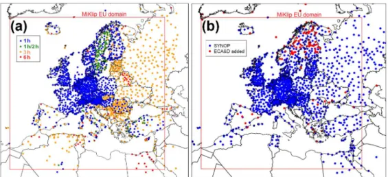
Figure 1.(a)SYNOP stations with hourly data in target DecReg EU domain for January 2010. The color code indicates the frequency of reports (between 1 and 6 h). The station records marked green contain hourly data but show gaps for the main dates: 00:00, 03:00, 06:00 UTC, etc.(b)SYNOP data forTavg(blue) in January 2001 and added ECA&D data using selection algorithm described in the text.
2.2 Hourly SYNOP reports
Figure 1a shows the distribution of SYNOP stations report-ing at least every 6 h (see color code for different frequen-cies) throughout the target domain for January 2010. In total, 2230 stations are found. Most of the regions in the target do-main (indicated by the red frame) are well covered; only for Africa are larger regions without data identified.
DailyTavgandVavgare derived by averaging the available hourly data, while assigning only half of the regular weight to the measurements at 00:00 UTC (of current and follow-ing day). Dependfollow-ing on the availability of hourly data, daily sample sizes vary between 25 (1-hourly, type 1), 16 (1-/2-hourly in Sweden, type 2), 9 (3-(1-/2-hourly, type 3) and 5 (6-hourly, type 4). To evaluate the consistency between daily means based on different sample sizes, these values were compared at stations with full daily records of 25 samples. In Fig. 2 daily means of types 3 and 4 in January 2001 are com-pared with type 1 for temperature (Fig. 2a1, a2) and wind speed (Fig. 2b1, b2) respectively. For temperature we find a high consistency of daily means even for type 4 (Fig. 2a2), with a standard deviation of the error of 0.21 K. For wind speed the precision in the determination of the daily mean decreases considerably with the number of samples per day (σ =0.40 m s−1for type 4). However, compared to the rel-atively high basic uncertainty of 0.5 m s−1 for wind speed data and the strong influence of, for example, local roughness conditions on the measurements, these potential discrepan-cies are found acceptable. For daily means of type 1 up to two missing or non-valid data in a daily record of 25 values were accepted. In the calculation of the daily means these gaps were filled by the mean of the two adjacent dates. Daily records of types 2–4 were rejected when missing values or inhomogeneities (see Sect. 2.4) occurred.
Figure 2.Accuracy of daily mean temperatures(a1, a2)and daily mean wind speeds(b1, b2)in January 2001 for different frequencies of observation (3 and 6 h) using 1-hourly data as reference. The standard deviations, denoted SD, are added to the histograms.
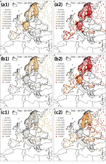
Figure 3.Differences of daily temperature data from SYNOP and ECA&D for January 2010 at stations with identical coordinates. Mean and maximum absolute daily deviation for minimum temper-ature(a1, a2), maximum temperature(b1, b2)and mean tempera-ture(c1, c2).
panels a1 and b1 the mean and maximum absolute differ-ences between dailyTminaccording to ECA&D and SYNOP are shown. For most of the countries, observation intervals in ECA&D (in many cases 24 h intervals, e.g., 00:00 to 00:00 UTC or 06:00 to 06:00 UTC; van den Besselaar et al., 2012) disagree with the 12 h period in SYNOP, which results in maximum daily deviations of more than 4 K at most of these stations in this winter month. In contrast, the ECA&D data of some countries in eastern and southern Europe are indicated to be derived consistently with SYNOP. Qualita-tively similar results are found forTmax(Fig. 3b1 and b2). For
Tavg(Fig. 3c1 and c2) the consistency of both data sources is high in the Netherlands and Germany (00:00 to 00:00 UTC in both archives). In all other countries, deviating intervals and/or calculation methods are apparent for ECA&D. Over-all, root mean square deviations (RMSD) of 1.9 K (Tmin), 1.7 K (Tmax) and 0.9 K (Tavg) are found in January 2010. In
spring and summer RMSD are usually smaller (0.8, 1.1 and 0.6 K forTmin,TmaxandTavg, respectively, in July 2010), as a result of increased insolation and more pronounced daily cycles.
To take account of this consistency problem, an algorithm was designed to include suitable data from the ECA&D archive, considering the density of SYNOP reports in each target area and by data comparison at identical stations (with same coordinates and altitudes). The differences at these sta-tions were used as indicator for the consistency in the target region for each day. Depending on the presence of SYNOP station data in a certain area, different thresholds for con-sidering or rejecting ECA&D station data were used (e.g., daily deviation required to be smaller than 1 K if at least one SYNOP station found within radius of 0.75◦(≈80 km)). In cases where no SYNOP data were available in an area of±3◦ (≈330 km) around a target ECA&D station and no comparison was possible in a somewhat larger area of±4.5◦ (≈500 km), ECA&D station data were included without any further testing. In such distances to other data points (about half of the ranges shown in Table 3; compare discussion on variogram ranges in Sect. 3.2), independent station data add essential information to the data field.
In Fig. 1b the station coordinates of a combined data set of SYNOP (blue) and ECA&D (red) forTavgin January 2001 are shown. The chosen ECA&D data add valuable informa-tion in Scandinavia, Spain and Greece. The total stainforma-tion num-ber is increased here by about 100.
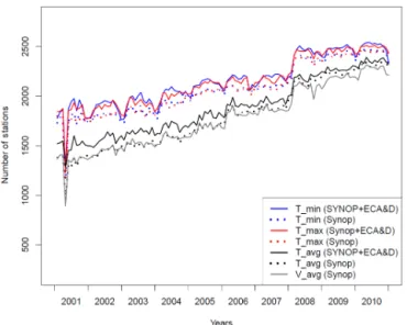
The temporal evolution during 2001–2010 of input data for the different parameters is illustrated in Fig. 4. The dot-ted lines show the fraction of SYNOP reports; the solid lines display the total number of station records used. For wind (grey curve) only SYNOP reports were used, as the num-ber of wind data archived in ECA&D is currently very low. Towards earlier years the availability of SYNOP reports de-creases. This decrease is considerable for the Scandinavian region and for many countries around the Mediterranean Sea (compare Fig. 1a and b). ECA&D data contribute especially in these early years. The availability of SYNOP data is usu-ally higher forTminandTmaxthan for the daily mean values
TavgandVavg.
2.4 Quality control and assurance
All input data (the hourly data of each day and the daily data of each month) were quality checked regarding different types of inhomogeneities: (1) outliers, (2) significant shifts in the time series, (3) constant data over longer intervals and (4) exceedance of climatological thresholds. In the follow-ing a closer description of the strategies for the example of hourly temperature data is given.
Figure 4.Temporal evolution of total input data used for the inter-polations 2001–2010 (see color code). The dotted curves show the basic number made up by SYNOP stations. The differences indi-cate the increase by the inclusion of ECA&D data. SYNOP data are used for the interpolations for wind speed only.
absolutely (adding notation 1) and relatively (divided by the standard deviation of the daily values without extremum, no-tation 2). Based on experiments with data of several exam-ple months, empiric thresholds were determined to decide whether a value is considered an outlier or not. Depending on the number of the daily values and the comparison of ab-solute vs. relative test value these thresholds range between 8 and 14 K for dt n1/dt x1and 4 and 8 for dt n2/dt x2.
For inconsistencies of types 2 and 3 a running standard de-viation (SDr) of five consecutive measurements is calculated. If the minimum of SDr(denoted SDnin the program) reaches zero, at least five identical values in a row are indicated. For a daily series of in total five values (6-hourly data), such an event is highly unlikely and therefore considered a result of erroneous data. In the case of hourly reports the threshold for a rejection is increased to nine identical values in a row. Our sample data showed that certain conditions in winter allow nearly unchanged temperatures over several hours. Also, the change of SDrfor each time step is recorded (the maximum difference is denoted dSDx) to identify sudden shifts in the common temperature level. Corresponding tests with data of several example months indicated clear inhomogeneities for dsdx above 7 K. Climatological thresholds were determined month-wise for 19 subregions using the full ECA&D archive for 1961–2010. The subregions were defined by combining countries of similar climate. For the Scandinavian countries and Russia an additional separation by latitude was applied. If subregions were insufficiently represented by ECA&D sta-tions, the upper and lower thresholds were slightly increased and decreased, respectively, to achieve realistic temperature limits. Additionally, an adjustment of temperature with
al-titude (assuming 0.65 K 100 m−1according to International Standard Atmosphere) is carried out to consider stations of high altitude possibly not represented by corresponding data of ECA&D.
In the case of wind speed, similar techniques, but with ad-justed thresholds, were developed to consider erroneous data. Concerning climatological thresholds, a global upper value of 65 m s−1for hourly data was defined. Here, an approach considering season and region is not helpful, as strong wind events can occur in all regions and throughout the year.
For the time series of daily values similar tests following the strategies for the hourly data are applied. This quality check is particularly important for the SYNOP extreme val-ues and for all ECA&D data because related hourly data are often not available. For stations where both extreme values and hourly raw data are available, a consistency check be-tween extremes based on these hourly data and the aggre-gated extremes (denoted “hrl” and “agg” in the following) is made (e.g., minimumTminaggis not expected to be above min-imum of corresponding hourly dataTminhrl). For temperature the consistency between the three parametersTmin,Tmaxand
Tavg(e.g.,Tminexpected to be smaller thanTavg) is checked for each day, if available.
The hourly data are also used to fill gaps in monthly time series of the extremes, if the overlap between, for exam-ple, Tminagg and Tminhrl is sufficiently long (more than 10 data points in a month) and the maximum discrepancy between these series is below 2 K. The estimates from the hourly raw data (e.g.,Tminhrl) are corrected by the mean deviation between both monthly time series to replace missing data of, for ex-ample,Tminagg. Similarly, ECA&D data are used for filling up incomplete monthly SYNOP series if the same coordinates and a high consistency (maximum deviation below 1 K) are found.
Figure 5.The seven regions used for temperature interpolation. The regional fields are finally merged using the regional weights (grey color scale). Stations used to calculate regional lapse rates are orange.
3 Interpolation procedure temperature
For temperature interpolation, a regression kriging approach (strategy proposed by Ahmed and de Marsily, 1987, and Odeh et al., 1995) adapted from Krähenmann et al. (2011) is used. The interpolation is done in four steps: a regression of station monthly means depending on three predictor parame-ters (altitude, continentality and zonal monthly mean temper-atures), followed by interpolation of the regression residuals using kriging to obtain gridded monthly means, a daily ad-justment of regression on altitude and, finally, the kriging of daily deviations from station monthly means.
The steps are performed separately in seven overlapping regions (see Fig. 5; 2.5◦,≈280 km, overlap). The separation roughly follows the climate classification after Köppen and Geiger (e.g., Sanderson, 1999), and thus relatively homoge-neous conditions for temperature are expected within each region. Compared to Krähenmann et al. (2011), slight modi-fications were made in the partitioning of the regions in order to adapt them to the DecReg domain dealt with in this work.
By considering regions instead of the whole domain, a better adjustment of the regression model and of the kriging param-eters (a closer description will follow) during interpolation is achieved. The regional temperature fields of the seven re-gions are finally merged by linear weighting in the overlap areas (see Fig. 5). This procedure ensures a continuous tran-sition of the data fields between two regions.
3.1 Regression
Figure 6.Predictor fields of altitude(a), continentality(b)and zonal monthly mean temperature (c; here January, based on climatology 1961–1990).
2005) is applied (see corresponding fields in Fig. 6).
T(x)=k0+k1×alt(x)+k2×con(x)+k3×zon(x)
+res(x), (1)
whereT(x) is temperature at stationx, alt is altitude, con is continentality index, zon is zonal mean temperature and res is residuum. These so-called predictor fields explain a ma-jor part of the spatial variation of monthly temperatures (Krähenmann et al., 2011). In order to receive a region-specific regression model, usually only data from stations within the core region (weight one; compare Fig. 5) are used to calculate the regression coefficients. Due to the relatively sparse data density in regions 1, 3 and 7, station data from the overlap areas are also considered here.
Among the three predictors, altitude is the most crucial be-cause temperature typically strongly depends on it and alti-tude changes in space occur on very small scales. Thus, linear regression against altitude can substantially improve the final interpolation results in regions with pronounced orographic characteristics. In a new setup applied in this work the depen-dency of monthly temperature from altitude is determined first and independently from the two other predictors on the basis of station data from mountainous areas. This strategy was chosen because height coefficients derived from the stan-dard multiple regression are potentially affected by strong horizontal temperature contrasts. For example, if mountain stations are concentrated in a part of a region with relatively low temperatures, lapse rates tend to be overestimated in the previous setup. Implausible lapse rates were diagnosed under such conditions, especially for the Scandinavian region. We could solve this issue with an independent regression step on altitude based on station data from valleys and moun-tains in relatively close distance. The orange dots in Fig. 5 mark stations used for this initial regression step. Depend-ing on the region, different criteria (minimum distance to coast, minimum altitude and regional weight) are applied to receive representative subsets. Due to the absence of station
data suitable for this approach in regions 3 and 7, the regres-sion coefficients for altitude determined in regions 2 and 6, respectively, are used here.
A second modification in the altitude regression setup was implemented in this work. Also daily temperature–altitude dependencies are estimated using the same strategy as above. In this way variations from day to day, which occur espe-cially in winter, can be considered.
Figure 7.Comparison of regression setups used to estimate temperature lapse rates for mean temperature in Scandinavia.(a)Stations used in different setups;(b)monthly lapse rates in 2010;(c)daily lapse rates for January 2010.
In comparison to the daily reference lapse rates (Fig. 7c, for January 2010), considerable deviations were found for both setups, with mean absolute deviations of 0.9 and 0.3 K 100 m−1 (T
min) for setup 1 (theoretical consideration, since no daily regression implemented in the previous work) and 2, respectively. Nevertheless, a clear improvement is achieved with the new setup in this problematic region. The periods of significant temperature inversions, indicated by the reference stations in the first half of the month, are not captured by the regression according to setup 1. However, it should be noted that none of the simple approaches shown here sufficiently describe the spatial variation of temperature in mountain regions during winter (see discussion in Sect. 7). Apart from this problematic region 2, no significant differ-ences in the results according to the two setups occurred in the tested months. In those regions absolute deviations from the reference lapse rates lie in the range of 0.1 K 100 m−1or below for monthly and daily data.
Latitudinal changes of the solar radiation as well as land– sea distribution and atmospheric dynamics (preferentially leading to a zonal air mass exchange) affect the predictor pa-rameter of the long-term zonal monthly mean temperature. Continentality reflects the buffering effect of the oceans on annual temperature changes. In contrast to altitude, these two predictor fields exhibit moderate spatial changes. Their po-tential for improving the interpolation is thus important in regions with a low observation density, e.g., in North Africa. Another modification compared to Krähenmann et al. (2011) is the use of station monthly means instead of cli-matological monthly values as input data for the monthly temperature analysis. In our work monthly hindcast periods are considered instead of current days (as in Krähenmann et al., 2011); therefore the values of the entire month are available. By using current monthly means as basis for the linear regression a potentially better adjustment of the
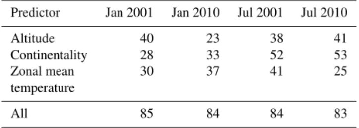
regres-Table 1.Whole-domain averages of spatial variance explained by single predictors (%) for monthly mean temperature and 4 tested months. In the bottom row the results for the multiple regression model involving all predictors are given.
Predictor Jan 2001 Jan 2010 Jul 2001 Jul 2010
Altitude 40 23 38 41
Continentality 28 33 52 53
Zonal mean 30 37 41 25
temperature
All 85 84 84 83
sion model to the mean weather conditions observed in this month is achieved and the amplitude of the regression resid-uals is reduced.
In Table 1 the predictive skills of the three predictors for monthly mean temperature are shown. Listed are the rela-tive explained variances in a regression with single predic-tors. The corresponding results for the multiple regression model is shown in the last row. All three parameters show a high capacity to predictTavg on a monthly basis. Overall, more than 80 % of the spatial variance can be explained by the three predictors.
3.2 Monthly and daily kriging
The monthly regression residuals (observations minus values according to regression model) are interpolated on a 0.011◦×
ful-filled, provided that most of the systematic variance has been removed by the regression step. However, a normal-score transformation (following Deutsch and Journel, 1998, attain-ing a standard normal distribution) is applied to the residuals prior to the interpolation. After interpolation and back trans-formation, block averaging is used to calculate the data on the final rotated target grid of 0.044◦×0.044◦(≈5 km). The sum of regression field and monthly residual field results in the monthly temperature field.
In the final step the differences between daily and monthly temperatures are interpolated following the same concept as above. Before this daily interpolation all daily anoma-lies are height-normalized using the daily regression coef-ficients (correcting deviations from monthly mean) for the temperature–altitude relationship determined in step one. The daily temperature field is eventually calculated as the sum of monthly temperatures, daily height-normalized resid-uals and the reversal of the height normalization.
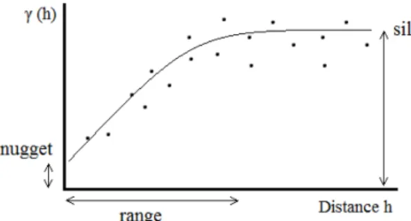
An important aspect in the interpolation using kriging is the adjustment of the kriging parameters (for details see, for example, Deutsch and Journel, 1998). These parameters estimate the change of correlation between nearby stations with distance. The related function considered in kriging is the semivarianceγ, describing half the variance between all pairs of data pointsZ(xi),Z(xi+h) at a certain distance,h, to each other.
γ(h)= 1
2N(h) NX(h)
i=1
{Z(xi)−Z(xi+h)}2 (2)
The corresponding graph, illustrated in Fig. 8, is called a variogram. The variogram parameters are sill (the maxi-mum semivariance observed in far distance from the origin), nugget (minimum semivariance observed at the origin) and range (the distance at which the semivariance levels off at the maximum). Stations outside the range are not expected to carry relevant information for a target point at the origin. The nugget, taking on values between zero and the sill, de-fines the noise of the data at the origin. Thus, it sets a basic uncertainty of all final gridded data in the considered region. This nugget effect can be understood as a result of measure-ment error and fluctuations below the spatial scale resolved by the stations. Different functions can be used to describe the change of the semivariance with distance. Here, a spher-ical model is assumed, following Krähenmann et al. (2011).
Several strategies of fitting the variogram function to the station data in each region were tested in this work. First, a “null” variogram is defined based on experiments with data from 4 example months (January 2001, July 2001, Jan-uary 2010, July 2010). Using cross validation, thus leaving out subsequently one data point and reproducing it based on the information from the remaining stations, different com-binations of the three parameters are tested. The parameter values performing best, define the “null” variogram. An au-tomated function for fitting variograms (Pebesma, 2004) is
Figure 8.Idealized variogram with the parameters nugget, sill and range (after Deutsch and Journel, 1998). See description in the text.
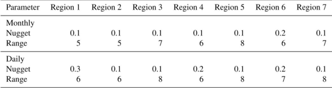
afterwards used to further optimize the variogram. Our tests showed that, on average, both the “null” variogram based on cross-validation results and the variogram based on the mated fitting perform equally well, but in rare cases the auto-mated fitting algorithm fails to determine reasonable results due to a missing convergence in the fitting based on least squares (Pebesma, 2004). In the final setup we decided to use the “null” variogram as a robust basis and allow a slight adjustment of the parameters in cases where clear differ-ences between the two models occur. The parameters nugget and range of this “null” variogram are listed in Table 3 for monthly and daily kriging ofTavg in the seven regions. The nugget values can be interpreted as percentage of the back-ground noise measured at the origin. ForTavgrelatively low nugget-to-sill ratios between 0.1 and 0.3 were determined. Thus, a relatively strong spatial dependence of the residual fields is indicated. The ranges, within which station data are correlated, are between 5 and 8◦on the rotated grid (≈550 to 900 km).
4 Interpolation procedure wind speed
For the interpolation of daily wind speed a new method based on the concept used for temperature was developed. Differ-ent predictor fields correlated with wind speed were tested and chosen. Again, the seven regions displayed in Fig. 5 are applied. In addition, a new region for the Alps is introduced (Fig. 9). The motivation for this new region will be outlined in the next section.
4.1 Regression
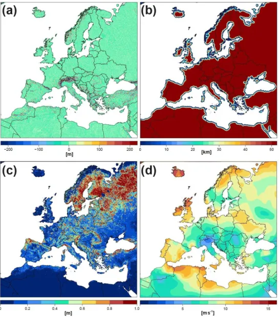
After testing a variety of potential predictor fields, four pa-rameters were chosen for the linear regression (see Fig. 10).
V(x)=k0+k1×exp(x)0.5+k2×ln (coa(x)+1)
+k3×ln 10 z0(x)
+k4×era(x)+res(x), (3)
Figure 9.Alpine region (denoted region 8 in the following) intro-duced for the interpolation of wind speed.
and res is residuum. The use of relative altitude (in the fol-lowing the term exposure will be used as a synonym) was motivated by Walter et al. (2006), who found good correla-tions with 10 m wind speed in Germany for altitude at a given point transformed to exposure by dividing it with the mean altitude of the surrounding area of 10 km×10 km. Here, we calculated corresponding fields on a 1 km grid using eleva-tion data (same sources as in Sect. 3.1) and applying a ra-dius of 5 km for the determination of surrounding mean al-titude. Block averages were calculated to obtain data for the final target grid of 5 km×5 km. For station data the exact altitude reported is used in comparison with the 1 km grid of mean altitudes described above. We tested different func-tions to find the most suitable relafunc-tionship between exposure and 10 m wind speed (e.g., linear, logarithmic and different power functions). On average, exposure to the power of 0.5 (equal to square root) showed highest correlations.
Coastal distance is also of high relevance for the mean wind speed in 10 m since the very low roughness across the sea surface, related to very low friction, leads to typi-cally stronger winds in the vicinity of coastlines. Our tests showed the best performance when using the logarithm of the coastal distance in the form ln(coa+1) and defining max-imum coastal distances (higher values are reduced to that constant) between 20 and 100 km. This maximum distance is chosen individually for each month and region on the basis of the lowest root mean square error (RMSE) for a regression on coastal distance.
Surface roughness describes the deviations of a surface from an ideal smooth form. On the Earth’s surface obsta-cles such as bushes, trees or buildings increase the surface roughness and thus affect the movement of air. According to theory the wind speed change with distance from the sur-face shows the following simplified dependency (under neu-tral stability conditions) on the roughness lengthz0(see, for
example, Holton and Hakim, 2012):
v(z)=v∗
κ ×ln z z0
, (4)
wherev(z) is wind speed at heightz, von Karman constant isκ and shear velocity isv∗. Based on this equation we ap-ply the roughness length in the regression step as ln(10/z0) because linear dependency onvis expected ifv∗is assumed constant (valid in the lowest 10 m considered here). Here, we use roughness length data in 1 km resolution derived from the global land cover data set GLC2000 (Bartholome and Bel-ward, 2005).
In addition to the three “static” predictor parameters above, the use of meteorological field data can provide valuable information for regions with low station coverage. Krähenmann and Ahrens (2013) showed that the inclusion of remote sensing data from satellite observations as a predic-tor in regression kriging substantially improves the gridding of surface temperature over the Iberian Peninsula. For wind speed, relevant satellite measurements of high quality are currently not available. However, air pressure fields, as the initial driving force of large-scale air movement, are well an-alyzed in weather models. Here, we tested ERA-Interim re-analysis data provided by the European Centre for Medium-Range Weather Forecasts (ECMWF). These data are avail-able in 6-hourly resolution on a reduced Gaussian grid with a grid point distance of approximately 80 km, from 1979 un-til today (Dee et al., 2011) at http://apps.ecmwf.int/datasets/ data/interim-full-daily/. In order to maintain independence from the other three predictors, corresponding model fields of geopotential height as well as the direct output for wind speed in pressure levels between 850 and 700 hPa (reflect-ing conditions in the nearly “free” atmosphere, undisturbed by surface impacts) were examined as predictor. Horizontal gradients derived from geopotential height and model wind speeds showed best correlations with surface station wind speed for the lowest tested level 850 hPa. This level corre-sponds with altitudes of around 1500 m; thus in high moun-tain areas like the Alpine region the data fields intersect with the land surface and therefore are affected by surface effects. In these cases an independence from the predictor fields of exposure and roughness length is not ensured. In the 700 hPa pressure level the influence of high mountains nearly van-ishes but the correlations are generally weaker. For the fi-nal regression setup we decided to use ERA-Interim wind fields at 850 hPa. Scalar wind speeds are derived from the two vector componentsuandv. Daily means are calculated in the same way as described in Sect. 2.2. For grid points above 1000 m reanalysis data are eliminated and afterwards re-estimated by the information of adjacent data points. Fi-nally, daily and monthly ERA-Interim scalar wind speed data fields are interpolated to the target DecReg grid using bilin-ear interpolation.
Figure 10.Predictor fields of exposure(a), coastal distance(b), roughness length(c), ERA-Interim mean scalar wind velocity in 850 hPa (d; here January 2001).
data on exposure and roughness length remains for areas like the Alps, the Atlas Mountains, the Caucasus and parts of Turkey. Thus, for the Alps, where a good coverage with sta-tion data is available, a new region (Fig. 9) was set up, for which regression on reanalysis wind speed is omitted. All grid points above 1500 m in this area receive regional weight one. An overlap to adjacent regions was determined and the regional weights of the adjacent regions were adjusted. Tests indicate a slight improvement of the overall explained vari-ance in 3 out of 4 tested months (January/July 2001/2010) for this new configuration.
The four predictors are used for the regression of the data of monthly mean wind speed. In contrast to temperature, wind speed data tend to produce a logarithmic distribution. Therefore, ratios between monthly wind data and the cor-responding area mean of the related region are considered.
Table 2.Whole-domain averages of the spatial variance explained by single predictors (%) for monthly mean wind speed and 4 tested months. The bottom row shows the result for the multiple regression model involving all predictors.
Predictor Jan 2001 Jan 2010 Jul 2001 Jul 2010
Exposure 24 20 18 17 Coastal distance 28 35 27 28 Roughness length 23 28 22 24 ERA-Interim 850 hPa 10 13 11 21
All 58 58 51 53
de-Table 3.Regional variogram parameters nugget (relative to sill) and range (◦rot. grid) based on experiments with temperature dataTavgof 4
example months (January 2001, July 2001, January 2010 and July 2010). Listed are the regional averages for monthly and daily interpolation.
Parameter Region 1 Region 2 Region 3 Region 4 Region 5 Region 6 Region 7
Monthly
Nugget 0.1 0.1 0.1 0.1 0.1 0.2 0.1
Range 5 5 7 6 8 6 7
Daily
Nugget 0.3 0.1 0.1 0.2 0.1 0.2 0.1
Range 6 6 8 6 8 7 8
Table 4.Regional variogram parameters nugget (relative to sill) and range (◦rot. grid) based on experiments with wind speed dataVavgof 4
example months (January 2001, July 2001, January 2010 and July 2010). Listed are the regional averages for monthly and daily interpolation.
Parameter Region 1 Region 2 Region 3 Region 4 Region 5 Region 6 Region 7 Region 8
Monthly
Nugget 0.8 0.5 0.7 0.3 0.6 0.6 0.8 0.3
Range 2 4 3 5 6 2 2 4
Daily
Nugget 0.7 0.4 0.5 0.3 0.4 0.4 0.5 0.7
Range 2 4 5 3 4 3 4 1
fine its core area. The test results of the monthly regression for the 4 example months are listed in Table 2. Each of the parameters explain a considerable part of the spatial variance ofVavg. Overall, around 55 % of the variance of the monthly mean is captured by the regression model. The values are somewhat lower than those obtained for temperature regres-sion. This can partly be explained by the high dependency of wind speed on local characteristics not captured by the regression.
Also, linear regression on a daily basis was tested, fo-cusing especially on the predictive skill of the daily ERA-Interim reanalysis data. Thereby we found good correlations between ERA-Interim and the daily observations. On aver-age, 31 % of daily variance could be explained by ERA-Interim over 4 tested months (same as above). Thus, an addi-tional regression step on a daily basis is applied using daily anomalies of ERA-Interim 850 hPa wind data from the cor-responding monthly means.
4.2 Monthly and daily kriging
Following the same scheme as described for temperature, the normal-score transformed residuals of the monthly regres-sion are interpolated using simple kriging. Again, a “null” variogram optimized on the basis of cross-validation exper-iments for 4 tested months (same as above) was determined for monthly and daily means in each region. The results are shown in Table 4. Compared to temperature the nuggets are somewhat larger and the ranges smaller. Thus, for wind speed the noise of the regression residuals at the origin of each
tar-get grid point is, on average, relatively large and the interpo-lation uncertainty relatively high. Regional signals vanish at distances of 2 to 6◦(≈220 to 670 km).
After normal-score back transformation the gridded monthly residuals are added to the gridded regression values and multiplied by the absolute mean wind speed of the con-sidered region (correcting the normalization applied before regression) to obtain the monthly field ofVavg.
In the daily kriging step the daily anomalies with respect to the monthly mean at each station are interpolated. Here, ratios instead of absolute deviations are considered, respect-ing the characteristics of wind speed distribution. As noted in Sect. 4.1, an additional regression with regard to daily ERA-Interim 850 hPa wind speed is performed prior to the interpo-lation. The final daily wind field is calculated involving the daily regression field, the back transformed daily anomaly ratios and the monthly field ofVavg.
4.3 Uncertainties of interpolation
Figure 11.Steps in the interpolation of daily mean temperature for 31 July 2010.(a)Monthly regression field;(b)monthly regression residu-als;(c)monthly mean temperature;(d)daily anomaly with respect to monthly mean temperature;(e)daily mean temperature;(f)interquartile range of daily mean temperature.
and kriging errors (kriging variance and semivariance at the origin) are combined according to error propagation to deter-mine total uncertainties. Finally, interquartile ranges (IQRs; range between 0.25 and 0.75 quantile, thus containing 50 % of the data) are recorded for all monthly and daily gridded data sets.
Figure 13.Detailed image of central Europe for(a)daily mean temperature (31 July 2010) and(b)daily mean wind speed (28 February 2010).
5 Results and discussion
5.1 Example outputs
In Fig. 11 the basic interpolation steps for the generation of the gridded field of daily mean temperature are illus-trated. The monthly field (Fig. 11c) is calculated as the sum of regression field (Fig. 11a) and the interpolated residuals (Fig. 11b). The interpolated daily anomalies (Fig. 11d) from the monthly data are used to determine the final grid of daily mean temperature (e, here for 31 July 2010). The uncertain-ties of the daily data are characterized by the IQR fields shown in Fig. 11f. In the central and northwestern part of the domain the quality is indicated to be very high, with IQR around 1.0 K. In other regions, where the coverage of station measurements is lower (compare Fig. 1), higher IQRs partly exceeding 3 K are recorded.
Corresponding results for daily mean wind speed on 28 February 2010 are shown in Fig. 12. Instead of absolute daily anomalies here the ratios to the monthly means are in-terpolated (Fig. 12d). Note that the intermediate step of daily regression on 850 hPa reanalysis winds (as for daily regres-sion on altitude in temperature scheme in Fig. 11) is not dis-played here. The uncertainties of the final daily wind speed data are relatively high in areas of high wind speeds. In con-trast to temperature, the dependency on the station density is lower because a considerable amount of the spatial vari-ability is not captured by station measurements and predictor fields (see discussion on the nugget effect in Sect. 3.2). To illustrate the small-scale characteristics of the interpolation products, the two example outputs for daily mean temper-ature and daily mean wind speed are displayed for central Europe in Fig. 13.
Figure 14.Relative explained variance for monthly mean wind speed and for the monthly mean of the three temperature param-eters (see color code) for 2001–2010.
5.2 Regression
Figure 15. Annual cycles (means 2001–2010) of relative explained variance for monthly mean temperature (a1, see color code of the parameters) and wind speed(b1)and corresponding spatial variability (1σ) before and after regression(a2, b2). All data are given as means over all regions. The error bars display the temporal standard deviation over the 10 years.
the 10 years no visible trend as a result of the trend in the number of station data is found. However, the curves indicate annual cycles caused by seasonal changes in spatial variance and/or the predictive capacity of the predictor fields.
This aspect is investigated more closely in Fig. 15. Here, annual cycles based on the statistics over the 10 years for EV and the spatial variability (standard deviation) of the raw data and the regression residuals are displayed. For temperature (Fig. 15a1, a2; see color code of the three parameters) a gen-erally higher spatial variability during winter is observed. For Tmaxan additional summer maximum is visible, the unex-plained variance even peaks in summer for this parameter. However, the high predictive capacity of the three predictors leads to a strong reduction of the residual variability for tem-perature.
For wind speed (Fig. 15b1, b2) similar annual cycles with winter maxima are indicated. After regression the remaining spatial variance is considerably reduced.
5.3 Interpolation – cross validation
For two years, 2001 and 2010, the quality of the final interpo-lation product is evaluated by applying “leave one out” cross validation (as defined in Sect. 3.2). Combining the cross-validation results for the monthly and the daily interpolation yields uncertainty estimates of the gridded data near each tar-get station. Figure 16 displays corresponding results for Jan-uary 2010 (Fig. 16a1, a2) and July 2010 (Fig. 16b1, b2) for daily mean temperature. Figure 16a1 and b1 show the mean absolute error of the 31 daily values at each station (see color code). The corresponding statistics over all days and stations are summarized in Fig. 16a2 and b2.
The RMSE is 1.68 K in January and 1.00 K in July. Thus, interpolation of mean temperature is, on average, consider-ably more accurate for the summer month considered here.
This finding is consistent with the relatively low variability of the regression residuals in summer (compare with Fig. 15). However, the regional distribution of the errors exhibits clear spatial differences: while in the north a tendency towards higher errors in winter is found, the southern regions reveal highest errors mainly in summer. This can possibly be ex-plained by the relatively low predictive capacity for night temperatures during cold winter periods (especially in com-plex terrain; e.g., cold air pools) and for day temperatures un-der high insolation in summer (affected by clouds, convective precipitation, coastal waters). This assumption is supported by the annual cycles of the regression residuals in Fig. 15. Especially during periods of temperature inversion in winter the simple linear regression approach on altitude is not capa-ble of reproducing the spatial temperature variation in moun-tainous regions satisfactorily (e.g., Frei, 2013). A discussion on this aspect will follow in Sect. 7. Overall, very accurate interpolation results are found in regions with a high obser-vation density and low topographic complexity.
Hofstra et al. (2008) have compared the skill scores for daily temperature interpolation results based on differ-ent methods. The RMSEs calculated in our study for the same domain are in the same range as found for the best-performing methods tested in Hofstra et al. (2008). For in-stance, the three-dimensional thin-plate splines method used (in combination with external drift kriging) for the E-OBS temperature grid record (Haylock et al., 2008) showed RM-SEs of 1.12 and 1.40 K for summer and winter half, respec-tively. A direct comparison between E-OBS grid data and the temperature data of our study is presented in Sect. 5.4.
Figure 16.Cross-validation results for daily mean temperature data in January 2010(a1, a2)and July 2010(b1, b2). The color code indicates the monthly mean of the daily absolute deviations. The histograms contain the full statistics of deviations over all days and stations.
(RMSE of 1.42 compared to 1.06 m s−1in July). However, seasonal differences can partly be attributed to the higher mean wind speeds occurring in January 2010 (mean over all stations: 3.37 compared to 3.05 m s−1in July). Relatively high absolute errors are found for stations in coastal and mountainous areas and thus at sites with high wind speeds. Nevertheless, the discrepancies diagnosed for highly exposed stations on the top of mountains typically show a systematic underestimation compared to the observed values (not illus-trated in the figure, as absolute deviations are given). Thus, systematic variance caused by the topography is not satis-factorily explained by the regression for areas of very high exposure.
In Fig. 18 the outcomes of cross validation are summarized for the entire annual cycles of 2001 and 2010 for the four pa-rameters: (a)Vavg, (b)Tavg, (c)Tminand (d)Tmax. The black and the blue curves illustrate the two cycles of daily RMSE. For comparison the time series of daily standard deviation over all station observations are displayed in brown and or-ange. In addition to the daily values curves of monthly means are shown. As indicated in Figs. 16 and 17, the interpola-tion accuracy is clearly higher during warmer seasons for the daily means of wind speed and temperature. Only forTmaxis a tendency towards higher errors in summer indicated. The interpolation quality is generally somewhat lower for the
ex-treme temperatures (see grey curves for Tavg added to the plots c and d for comparison). The temporal averaging used to calculate daily means leads to a reduction of unexplained variance (compare with in Fig. 15a2) and thus increases the accuracy of the interpolation.
The variability curves in Fig. 18 can be interpreted as the RMSE for the simple assumption in which the mean over all station data is assigned to each station location. Thus, the dif-ference between lower and upper curves can be understood as a measure for the skill of the interpolation method. For wind speed this skill is much lower than for temperature due to the large fraction of unexplained variance.
be-Figure 17.Cross-validation results for daily mean wind speed data January 2010(a1, a2)and July 2010(b1, b2). The color code indicates the monthly mean of the daily absolute deviations. The histograms contain the full statistics of deviations over all days and stations.
tween observations and interpolation results is found. Only for Tminare significantly underestimated variances detected during certain periods. For wind speed the relative variances fluctuate around a level slightly below 0.7 (outliers for sin-gle days in April 2001 due to very low number of station data). This low variance ratio is caused by the high degree of unexplained variance observed on very small scales (nugget effect, Sect. 4.2). The reproduction of a data value at a cer-tain station by a weighted average of surrounding values with a large spread leads, on average, to a reduced signal at this station.
5.4 Comparison with E-OBS grid data
To assess the characteristic of the temperature data set in comparison with the daily E-OBS grid data (version 13.0; Haylock et al. (2008); www.ecad.eu/download/ensembles/ ensembles.php), the data fields of daily mean temperature were compared for 2010. To meet the lower resolution of E-OBS (0.22◦), the DecReg data were transferred to the E-OBS grid using first-order conservative remapping. For 31 January 2010 (Fig. 20) we find very similar temperature fields ofTavg for DecReg (Fig. 20a) and E-OBS (Fig. 20b) in most parts of the domain. However, the difference field DecReg minus E-OBS (Fig. 20c) reveals major discrepancies in Russia and in mountain regions around the Mediterranean Sea.
As shown in Sect. 2.3, deviating observation intervals and/or calculation methods (in the case ofTavg) occasionally cause considerable differences of the daily station data used for the two data sets (mainly ECA&D for E-OBS, mainly SYNOP for DecReg), especially in winter. The correspond-ing comparison (SYNOP minus ECA&D at stations with identical coordinates) for the investigated day is shown in Fig. 20d. The differences of the grid data found in eastern Eu-rope are well explained by the deviating source data. In con-trast, the station data in the Mediterranean region are found consistent for this day. Here, differences in the assumed lapse rates lead to varying results for grid cells of high altitudes. Since in E-OBS these dependencies are calculated locally (see Haylock et al., 2008), there is a potentially better re-flection of small-scale changes; however, this strategy lacks robustness in cases of missing representation by local sta-tion data. The maps of mean daily deviasta-tion (Fig. 20e) and mean absolute daily deviation (Fig. 20f) between DecReg and E-OBS indicate persistent differences in mountain re-gions around the Mediterranean.
Figure 18.Annual cycle of daily RMSE according to cross validation for 2001 (black) and 2010 (blue) for(a)mean wind speedVavg, (b)mean temperatureTavg,(c)minimum temperatureTminand(d)maximum temperatureTmax. For comparison, the daily standard deviation
over all station observations is displayed in brown (2001) and orange color (2010). Corresponding curves of monthly means are added to all data. In panels(c)and(d)the RMSE data forTavgare displayed in grey color for comparison.
averaging in the same way, as described in Sect. 2.2. The data fields were interpolated to the E-OBS and the DecReg grid using bilinear remapping. All grid points at altitudes near the level of 850 hPa – a range between 1200 and 1800 m was defined – were compared with ERA-Interim. To cor-rect for temperature differences caused by height deviations, observational grid data were normalized (for each day and grid point) to the actual geopotential height at 850 hPa (from daily ERA-Interim field) by assuming linear lapse rates de-termined on the basis of the eight surrounding grid cells.
The outcomes of this comparison for January 2010 are shown in Fig. 21. For the difference E-OBS minus ERA-Interim at 850 hPa (Fig. 21a), mean daily deviations vary between−3 and+8 K. A clear overestimation of mountain temperatures is indicated for the Atlas Mountains, the Sierra Nevada (southern Spain) and for the French Alps.
Figure 19.Time series of the ratio of spatial variance of interpo-lated vs. observed station data for the years 2001 and 2010 based on cross validation. The color code indicates the parameters and years.
single grid points the consistency between E-OBS and ERA-Interim is relatively high, with only occasional negative bi-ases above 3 K occurring in winter months. The DecReg data show constant negative biases compared with ERA-Interim of around 2–3 K at the grid points in Morocco, Spain and Syria. For the other mountain regions the data agree rela-tively well, except for single winter months with clear nega-tive biases.
In a further analysis the ERA-Interim temperatures at 850 hPa were compared with SYNOP station data to evalu-ate the representativeness of the model data (initial resolution of≈80 km) for the relatively fine grids of E-OBS (≈25 km) and DecReg (≈5 km). The data of up to three suitable moun-tain stations (heights between 1200 and 1800 m) within a ra-dius of 2.5◦ (≈280 km) around the single grid points ana-lyzed above were compared with the nearest ERA-Interim grid point (interpolated; 0.044◦). Similarly to the procedure above, station temperatures were normalized to the 850 hPa geopotential height for each day (based on lapse rates deter-mined from DecReg). The results of this comparison in the environment of the single grid points are shown in Fig. 21e. The consistency between station data and ERA-Interim (no station data available for grid points in Spain) is very high for most time of the year 2010. Daily deviations are typically within the range of±2 K. For the grid points in Norway and Turkey, similar negative biases are observed as for E-OBS and DecReg for the winter months (Fig. 21c and d). Thus, the reanalysis data tend to be incorrect or not representative in some of the mountain regions during winter. Reversely, the observational grid data of E-OBS and DecReg are indicated to be consistent with the observations for these areas, even in winter.
Overall, E-OBS and DecReg mountain temperatures at around 1500 m are in an acceptable agreement with ERA-Interim reanalysis data and station observations. However, the interpolation procedure used for E-OBS fails to repro-duce temperature changes with altitude sufficiently in areas without suitable observations. The regression approach pre-sented in this study is indicated to be slightly more reliable in these problematic areas but is incapable of representing lo-cal deviations from the lapse rate determined for each region. Additionally, both approaches are incapable of dealing with nonlinear lapse rates.
Regarding the observation intervals of the daily E-OBS data, no consistency throughout the domain is ensured, which is a result of deviating procedures applied by the national weather agencies providing data to ECA&D. The SYNOP input data used in DecReg are based on the same daily in-tervals. Thus, potential discontinuities of temperature fields near national borders are avoided and comparability with model data for defined intervals ensured.
Apart from the causes discussed above, differences in the distribution of the input station data used in E-OBS and De-cReg can also lead to deviating grid data. This aspect is im-portant for regions where the density of stations is generally low, as observed around the Mediterranean Sea, especially in the early years of the decade (compare Fig. 1).
5.5 Evaluation of uncertainty estimates
As mentioned in Sect. 4.3, uncertainty fields based on re-gression error and kriging variance were determined for each monthly and daily data field. In the following, a compari-son of these estimates with the findings from cross valida-tion is presented. We use daily cross-validavalida-tion results (as shown in, for example, Fig. 16) and the monthly mean of daily IQR at the nearest adjacent grid points. For each station the number of interpolated data within the IQR error interval is counted for the 2 example months January and July 2010. The results of this experiment are displayed in Fig. 22 for daily mean temperature. Blue colors indicate point data for which more daily data lie outside the range of error than ex-pected. Grey dots mark data for which the monthly statistic fairly agrees with the definition of IQR (50±10 %). Loca-tions with more accurate data than indicated by the IQR are colored red. Additionally, corresponding frequency distribu-tions are displayed for the 2 months (Fig. 22a2, b2).
Figure 20.Comparison of daily temperature grid data from DecReg and E-OBS for January 2010:(a)DecReg daily mean temperature (Tavg) 31 January 2010;(b)E-OBSTavg31 January 2010;(c)DecReg minus E-OBSTavg31 January 2010;(d)SYNOP minus ECA&D
Tavg31 January 2010;(e)mean daily deviations DecReg minus E-OBSTavgJanuary 2010;(f)mean absolute daily deviations DecReg minus
E-OBSTavgJanuary 2010.
of a relatively low or relatively high local variability of the input data are not considered in the kriging variance. This measure mainly depends on the variogram parameters – re-flecting average changes of the correlation between adjacent data values with distance – and the station density. For cer-tain months the basic variogram parameters determined for each region (“null” variogram, see Sect. 3.2) can deviate
sig-nificantly from the real data characteristics in that specific month. The restriction of the automated variogram fitting (to avoid unstable variogram models, Sect. 3.2) can lead to mean IQR estimates deviating from the mean errors based on cross validation.
uncer-Figure 21.Comparison of daily temperature grid data at altitudes of around 1500 m from DecReg and E-OBS with ERA-Interim 850 hPa temperatures for January 2010:(a)E-OBS minus ERA-Interim mean deviations of daily mean temperatures (Tavg);(b)DecReg minus
ERA-Interim mean deviations of dailyTavg;(c)annual cycle of E-OBS minus ERA-Interim deviations of dailyTavg(monthly mean and standard
deviation) at single grid points encircled in panel(a);(d, e)same as in panel(c)but for the comparison DecReg minus ERA-Interim and SYNOP minus ERA-Interim, respectively.
tainty range. However, also here the spatial variation is very high. In contrast to temperature, the distribution of signifi-cantly outlying data values is less systematic for wind speed (Fig. 23a2, b2). This can be explained with its relatively high spatial variability on small scales.
6 Summary
In this work interpolation schemes for daily station data of minimum, maximum and mean temperature as well as daily mean wind speed in 0.044◦(≈5 km) resolution for Europe (rotated grid, virtual North Pole at 39.25◦N, 162◦W) are presented. To achieve a high data consistency, temperature extremes are based on the same 12 h intervals of night (18:00 to 06:00 UTC) and day (06:00 to 18:00 UTC), and a
consis-tent 24 h interval starting at 00:00 UTC is used for the calcu-lation of daily means. A regression kriging approach using predictors altitude, continentality and zonal monthly mean temperature, based on the work by Krähenmann et al. (2011), is applied for the temperature parameters. Modifications and further developments were implemented to adapt the exist-ing routine to the special demands of our project. For wind speed a new regression kriging procedure involving the pre-dictor variables exposure, coastal distance, roughness length and 850 hPa ERA-Interim reanalysis wind speeds was devel-oped.
temper-Figure 22. Comparison of cross-validation results with gridded uncertainty estimates for daily mean temperature in January 2010(a1)
and July 2010(b1): fraction of interpolated daily data at stations within nearest-neighbor gridded IQR (interquartile range). Blue indicates an underestimation; red indicates an overestimation of the uncertainty. In panels(a2)and(b2)corresponding frequency distributions are displayed.
atures and the data of the ECA&D archive, detailed quality control procedures were developed. In order to maintain con-sistency with SYNOP, a selection algorithm, controlling the integration of ECA&D data in regions where SYNOP data are sparse and consistency between the two sources is high, was implemented.
For the time period 2001–2010 the spatial variation of the monthly means can be well explained by the predictors. We obtain relative explained variances in the range of 80–90 % for the temperature parameters and about 50–60 % for wind speed.
Cross validation is performed for the years 2001 and 2010 to assess the quality of the daily interpolation products. For daily mean temperature, RMSEs of about 1–2 K are diag-nosed. The accuracy for the daily extremes is typically lower, with values around or slightly below 2 K. In winter interpola-tion accuracies tend to be reduced compared to summer. For daily maximum temperatures an additional summer reduc-tion in gridding accuracy is detected. The RMSE for daily mean wind speed lies in the range of 1–1.5 m s−1. Here, an annual cycle, with the higher values occurring in winter, is also indicated.
Concerning the conservation of spatial variance, very good performance is found for the temperature parameters. In the interpolation products 90–100 % of the observed variance is typically preserved. Only for minimum temperature are at times lower values recorded. For daily wind speed, a fraction of 60–80 % of the original variance is preserved after interpo-lation. The relatively high degree of unexplained small-scale variance leads to a smoothing of the wind data.
The cross-validation results are also used to evaluate the quality of the gridding uncertainty based on kriging variance and regression errors. On average, a reasonable consistency between these data is found. Nevertheless, temporal and spa-tial variations of uncertainty occurring on small scales are not adequately reflected in the gridded uncertainties.
Figure 23. Comparison of cross-validation results with gridded uncertainty estimates for daily mean wind speed in January 2010(a1)
and July 2010(b1): fraction of interpolated daily data at stations within nearest-neighbor gridded IQR (interquartile range). Blue indicates an underestimation; red indicates an overestimation of the uncertainty. In panels(a2)and(b2)corresponding frequency distributions are displayed.
850 hPa satisfactorily in areas without sufficient data from mountain stations.
7 Conclusions
The regression kriging approaches used in this work for the interpolation of daily temperature and wind speed observa-tions on a grid size of 0.044◦ (≈5 km) show good perfor-mance in terms of accuracy and variance preservation. With the inclusion of suitable predictor variables small-scale char-acteristics of the meteorological parameters can be well cap-tured.
For the dependency of temperature on altitude more reli-able regression results are obtained by performing this re-gression separately and on the basis of representative sta-tions. Also, day-to-day variations of this dependency are considered in the new setup used in this study. Neverthe-less, the linear regression approach applied to the relatively large areas of each region is not capable to reflect nonlinear vertical temperature changes and spatial differences of this parameter within a region. More complex approaches con-sidering this issue in the calculation of high-resolution grid
data in mountainous regions have been published (e.g., Frei, 2013). However, these specialized strategies require the pres-ence of stations representative for a certain area and altitude level. For the relatively large domain dealt with in our work, where many mountain regions are insufficiently represented by station data, the inclusion of radiosonde data might offer a promising strategy in this respect.
Concerning the regression of wind speed, a considerable part of spatial variance on a monthly basis (40–50 %) re-mains unexplained by the predictors used in this work. For predictor fields of exposure, coastal distance and roughness length it would be more realistic to take into account the cur-rent wind direction and local predictor conditions determined for this wind direction. This strategy would introduce further complexity in the calculations. However, the percentage of variance explained by predictors as well as the final interpo-lation accuracy could likely be increased.
enormous increase in computing time. Thus, the determina-tion of accurate uncertainty estimates remains an issue for data sets of high resolution in space and time.
However, users of these grid data are recommended to con-sider the IQR uncertainty fields provided in separate files in their analyses. Especially in parts of North Africa the uncer-tainties are usually very high due to very sparse observations. To deal with this issue, IQR thresholds tolerable for a specific analysis could be defined to exclude regions with less reliable data.
8 Data availability
The data sets presented in this article are published at doi:10.5676/DWD_CDC/DECREG0110v2 (Brinckmann and Bissolli, 2016). Elevation data of the DecReg grid are available at ftp://ftp-cdc.dwd.de/pub/CDC/help/.
Acknowledgements. The authors would like to acknowledge the Bundesministerium für Bildung und Forschung (BMBF) for funding this project. The colleagues in the department Regional Climate Monitoring at Deutscher Wetterdienst (DWD) are ac-knowledged, especially Maya Körber and Andrea Kreis for their support in technical issues related to UNIX and database queries. We also thank our partners participating in the DecReg project for the fruitful cooperation during the 26 months. Furthermore, the E-OBS data set from the EU-FP6 project ENSEMBLES (http://ensembles-eu.metoffice.com) and the data providers in the ECA&D project are acknowledged (http://www.ecad.eu).
Edited by: G. König-Langlo
Reviewed by: two anonymous referees
References
Ahmed, S. and de Marsily, G.: Comparison of geostatistical meth-ods for estimating transmissivity using data on transmissiv-ity and specific capactransmissiv-ity, Water Resour. Res., 23, 1717–1737, doi:10.1029/WR023i009p01717, 1987.
Bartholome, E. and Belward, A. S.: GLC2000: a new ap-proach to global land cover mapping from Earth ob-servation data, Int. J. Remote Sens., 26, 1959–1977, doi:10.1080/01431160412331291297, 2005.
Brinckmann, S. and Bissolli, P.: DecReg/MiKlip gridded data of near-surface temperature (2 m) and wind speed (10 m) in Europe for the period 2001–2010, Version v002, DWD Climate Data Center, doi:10.5676/DWD_CDC/DECREG0110v2, 2016. Dee, D. P., Uppala, S. M., and Simmons, A. J. E. A.: The
ERA-Interim reanalysis: configuration and performance of the data assimilation system, Q. J. Roy. Meteor. Soc., 137, 553–597, doi:10.1002/qj.828, 2011.
Deutsch, C. V. and Journel, A.: GSLIB: Geostatistical Software Li-brary and User’s Guide, 2nd edn., Oxford University Press, New York, USA, 1998.
Frei, C.: Interpolation of temperature in a mountainous region using nonlinear profiles and non-Euclidean distances, Int. J. Climatol., 34, 1585–1605, doi:10.1002/joc.3786, 2013.
Gerth, W.-P. and Christoffer, J.: Windkarten von Deutschland, Me-teorol. Z., 3, 67–77, 1994.
Gorczynski, L.: Sur le calcul du degré de continentalisme et son application dans la climatologie, Geografiska Annaler, 2, 324– 331, 1920.
Hansen, J., Ruedy, R., Sato, M., and Lo, K.: Global sur-face temperature change, Rev. Geophys., 48, RG4004, doi:10.1029/2010RG000345, 2010.
Haylock, M. R., Hofstra, N., Klein Tank, A. M. G., Klok, E. J., Jones, P. D., and New, M.: A European daily high-resolution gridded data set of surface temperature and pre-cipitation for 1950–2006, J. Geophys. Res., 113, D20119, doi:10.1029/2008JD010201, 2008.
Hogewind, F. and Bissolli, P.: Operational maps of monthly mean temperature for WMO Region VI (Europe and Middle East), Ido-jaras, 115, 31–49, 2011.
Hofstra, N., Haylock, M. R., New, M., Jones, P. D., and Frei, C.: Comparison of six methods for the interpolation of daily European climate data, J. Geophys. Res., 113, D21110, doi:10.1029/2008JD010100, 2008.
Holton, J. R. and Hakim, G. J.: An Introduction to Dynamic Mete-orology, 5th edn., Academic Press, Waltham, MA, USA, 2012. Klein Tank, A. M. G., Wijngaard, J. B., Können, G. P., Böhm, R.,
Demarée, G., Gocheva, A., Mileta, M., Pashiardis, S., Hejkr-lik, L., Kern-Hansen, C., Heino, R., Bessemoulin, P., Müller-Westermeier, G., Tzanakou, M., Szalai, S., Pálsdóttir, T., Fitzger-ald, D., Rubin, S., Capaldo, M., Maugeri, M., Leitass, A., Bukan-tis, A., Aberfeld, R., van Engelen, A. F. V., Forland, E., Mietus, M., Coelho, F., Mares, C., Razuvaev, V., Nieplova, E., Cegnar, T., Antonio López, J., Dahlström, B., Moberg, A., Kirchhofer, W., Ceylan, A., Pachaliuk, O., Alexander, L. V., and Petrovic, P.: Daily dataset of 20th-century surface air temperature and precip-itation series for the European Climate Assessment, Int. J. Cli-matol., 22, 1441–1453, doi:10.1002/joc.773, 2002.
Krähenmann, S. and Ahrens, B.: Spatial gridding of daily maximum and minimum 2-m temperatures supported by satellite observations, Meteorol. Atmos. Phys., 120, 87–105, doi:10.1007/s00703-013-0237-9, 2013.
Krähenmann, S., Bissolli, P., Rapp, J., and Ahrens, B.: Spatial grid-ding of daily maximum and minimum temperatures in Europe, Meteorol. Atmos. Phys., 114, 151–161, doi:10.1007/s00703-011-0160-x, 2011.
Li, J. and Heap, A. D.: A review on spatial interpolation methods for environmental scientists, Geoscience Australia, 15, 585–596, doi:10.1127/0941-2948/2006/0162, 2008.
Luo, W., Taylor, C., and Parker, S. R.: A comparison of spatial in-terpolation methods to estimate continuous wind speed surfaces using irregularly distributed data from England and Wales, Int. J. Climatol., 28, 947–959, doi:10.1002/joc.1583, 2008.
Matheron, G.: Principles of geostatistics, Econ. Geol., 58, 1246– 1266, 1963.
Morice, C. P., Kennedy, J. J., Rayner, N. A., and Jones, P. D.: Quantifying uncertainties in global and regional tempera-ture change using an ensemble of observational estimates: the HadCRUT4 data set, J. Geophys. Res., 117, D08101, doi:10.1029/2011JD017187, 2012.
Odeh, I. O. A., McBratney, A. B., and Chittleborough, D. J.: Further results on prediction of soil properties from terrain attributes: het-erotropic cokriging and regression-kriging, Geoderma, 67, 215– 226, doi:10.1016/0016-7061(95)00007-B, 1995.
Pebesma, E. J.: Multivariable geostatistics in S: the gstat package, Comput. Geosci., 30, 683–691, doi:10.1016/j.cageo.2004.03.012, 2004.
Rohde, R., Muller, R., Jacobsen, R., Perlmutter, S., Rosenfeld, A., Wurtele, J., Curry, J., Wickham, C., and Mosher, S.: Berkeley Earth Temperature Averaging Process, Geoinfor. Geostat.: An Overview 1, 1–13, doi:10.4172/2327-4581.1000103, 2013. Sanderson, M.: The classification of climates from
Pythago-ras to Koeppen, B. Am. Meteorol. Soc., 80, 669–673, doi:10.1175/1520-0477(1999)080<0669:TCOCFP>2.0.CO;2, 1999.
Smith, T. M., Reynolds, R. W., Peterson, T. C., and Lawrimore, J.: Improvements to NOAA’s historical merged land–ocean surface temperature analysis (1880–2006), J. Climate, 21, 2283–2296, doi:10.1175/2007JCLI2100.1, 2008.
Stahl, K., Moore, R. D., Floyer, J. A., Asplin, M. G., and McK-endry, I. G.: Comparison of approaches for spatial interpolation of daily temperature in a large region with complex topography and highly variable station density, Agr. Forest Meteorol., 139, 224–236, doi:10.1016/j.agrformet.2006.07.004, 2006.
van den Besselaar, E. J. M., Klein Tank, A. M. G., van der Schrier, G., and Jones, P. D.: Synoptic messages to ex-tend climate data records, J. Geophys. Res., 117, D07101, doi:10.1029/2011JD016687, 2012.
Walter, A., Keuler, K., Jacob, D., Knoche, R., Block, A., Kot-larski, S., Müller-Westermeier, G., Rechid, D., and Ahrens, W.: A high resolution reference data set of German wind velocity 1951–2001 and comparison with regional climate model results, Meteorol. Z., 23, 585–596, 2006.