RBRH, Porto Alegre, v. 22, e49, 2017 Scientiic/Technical Article
http://dx.doi.org/10.1590/2318-0331.0217160021
Prediction of the bedforms generated by density currents based on luvial phase
diagrams
Previsão das formas de fundo geradas por correntes de densidade a partir de diagramas de fases fluviais
Débora Karine Koller1, Ana Luiza de Oliveira Borges1, Eduardo Puhl1 and Rafael Manica1
1Universidade Federal do Rio Grande do Sul, Porto Alegre, RS, Brazil
E-mails: [email protected], [email protected], [email protected], [email protected]
Received: November 03, 2016 - Revised: April 27, 2017 - Accepted: May 30, 2017
ABSTRACT
Density currents, whose movement takes place by the density difference between the low and the ambient luid around it, can interact with the substract generating bedforms similar to the luvial environments. However, there are no speciic bedform phase diagrams capable to predict this type of phenomenon. This study aims to compare the prediction of luvial bedforms phase diagram with those generated by experimental saline currents. Bedforms were generated in two-dimensional tilting plexiglass lume submerged in a larger tank illed with water with three different mobile beds and varied values of discharge and salt concentration. It was observed three
types of bedform (lower plane bed, ripples and dunes), which, with the concomitant calculation of hydrodynamic parameters (mean
velocity, energy and mobility) allowed the use of the phase diagram. It was observed that the luvial phase diagrams did not present
good predictions for bedforms generated by density currents. This fact is associated to the hydrodynamics differences (velocity and
concentration proiles) and the limitation of the dimensional parameters in the extrapolation of results. Therefore, it is indicated the
need to draw up a proper phase diagram to density currents.
Keywords: Density current; Bedforms; Physical modeling; Mobile bed; Bedform phase diagram.
RESUMO
As correntes de densidade, cujo movimento ocorre pela diferença de massa especíica entre o escoamento e o luido ambiente ao seu redor, podem interagir com o substrato gerando formas de fundo, similares às encontradas em ambientes luviais. Entretanto não existem diagramas de previsão especíicos correspondentes para esse tipo de fenômeno. Assim, este trabalho visa comparar a ocorrência das formas de fundo luviais previstas nos diagramas de previsão com aquelas geradas por correntes de densidade salinas
obtidas experimentalmente. As formas de fundo foram geradas em um canal bidimensional de declividade variável, preenchido por
água, com três composições de leito móvel e diferentes valores de vazão, massa especiica e inclinação. Três formas de fundo foram identiicadas (leito plano inferior, ondulações e dunas), as quais, juntamente com o cálculo de parâmetros hidrodinâmicos permitiram a utilização dos diagramas luviais. Veriicou-se que os diagramas luviais não apresentaram boas previsões das formas de fundo geradas por correntes de densidade. A esse fato são atribuídas as diferenças hidrodinâmicas dos escoamentos (peris de velocidade e concentração) e, também, à limitação dos parâmetros dimensionais na extrapolação dos resultados. Dessa forma, indica-se a necessidade
de se elaborar um diagrama de previsão próprio adaptado a estas correntes.
INTRODUCTION
Bedforms are sedimentary features observed in several
environments, such as eolian, luvial, and deep sea, generated by the stresses applied by certain lows.
The understanding on processes of erosion, transport and sedimentation of the grains, which makes up the generation and development of bedforms has been extensively approached
by luvial hydrology for many decades (HJÜSTROM, 1935 apud
GRAF, 1971; SHIELDS, 1936; RAUDKIVI, 1997; CARTIGNY; POSTMA, 2016, among others).
Each type of low develops speciic hydraulic characteristics
(e.g., velocity and concentration) that are eventually transmitted to
the mobile bed over which it lows, such as generating bedforms.
Thus, the study of these forms (plane bed, ripples, dunes, and antidunes - SIMONS; RICHARDSON, 1961) can be used as a tool in the understanding of hydraulic processes based on existing geological records in nature, such as turbidites (MIDDLETON, 1993), which are relevant to the oil industry. These deposits may be associated with density currents, whose movement occurs due
to the density difference between the low and the surrounding luid (MIDDLETON, 1966; SIMPSON, 1997).
Mechanisms that govern the generation and migration of bedforms by density currents in marine environments are poorly
understood because of the dificulty of direct observation, the
limited number of experimental studies, and the complexity of
these lows in relation to the luvial (FEDELE; GUENTZEL;
HOYAL, 2009). Consequently, some studies (PARKER et al., 1987;
RAUDKIVI, 1997; PUHL, 2012; CARTIGNY; POSTMA, 2016, among many others) merge or even adapt existing knowledge about
bedforms generated by luvial lows assuming similar emergence
and development between the two.
Some small scale experiments already performed with saline density currents or composed of suspended sediments (turbidity currents) analyzed the morphology of the mobile bed for different
low regimes (subcritical, critical, and supercritical). In general, lower plane beds, ripples, and dunes occur in subcritical lows
(KNELLER; BENNETT; MCCAFFREY, 1997), whereas upper plane beds and antidunes are formed spontaneously in moving beds
after supercritical lows (HAND, 1974; WINTERWERP et al., 1992;
SPINEWINE et al., 2009; FEDELE; HOYAL; DRAPER, 2011). Furthermore, Fedele, Guentzel and Hoyal (2009) identiied a new type of bedform generated by density currents whose genesis resembles antidunes and whose development is similar to lower
water-depth wavelength antidunes with migration in the low
direction (unlike what usually occurs in free surface lows), due to the interaction at the interface between the shape and the low.
In general, the prediction of bedforms by density currents
is made based on stability diagrams (RAUDKIVI, 1990; CHANG, 1988) developed for luvial bedforms despite differences between the hydraulic and sedimentological processes present in each case.
Among the several existing diagrams, this study analyzed the following four: Simons and Richardson (1961), Southard and Boguchwal (1990), Athaullah (1968 apud JULIEN, 1998), and Van
den Berg and Van Gelder (1993).
Simons and Richardson (1961) were the pioneers in the attempt to predict the types of bedforms, seeking to relate data from average grain size (d50) with low’s energy (τU), establishing zones of probable occurrence of plane bed (lower and upper), ripples, dunes, and antidunes. Southard and Boguchwal (1990) developed one of the most used diagrams to predict bedforms, simple use and interpretation, which involves the direct plot of the average stream velocity and the average sediment size present in the bed.
Athaullah’s diagram (1968 apud JULIEN, 1998) correlates the dimensionless Froude number (Fr) and the ratio between hydraulic radius (Rh) and average grain size (d50), separating bedforms into
zones of subcritical, critical, and supercritical low regimes. Van den Berg and Van Gelder diagram (VAN DEN BERG; VAN GELDER,
1993) compares the dimensionless mobility parameter (θ’) and the average dimensionless grain size parameter (d50*). The importance of the use of dimensionless parameters is emphasized by the last two authors, in the comparison of results among studies so that the scale effects present in the phenomenon be considered.
In view of the above, the present study applied an
experimental methodology to generate bedforms by density currents and related the obtained results with the three mentioned
luvial phase diagrams in order to verify the applicability of these
diagrams to the bedforms generated by density currents.
METHODOLOGY
Apparatus and experimental description
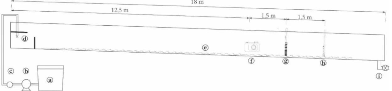
Experiments were performed in an 18 m long acrylic lume and rectangular cross section of 0.2 m x 0.5 m with a variable slope
(Figure 1), built into a long masonry tank (25 m long and 0.74 x 1 m cross section).
Figure 1. Test coniguration (a) Reservoir for mixture preparation (b) Pump (c) Flow meter (d) Density current input (e) Mobile bed
Prior to each test, the bottom of the acrylic lume was illed
with the sediment chosen to compose the mobile bed. Tests were
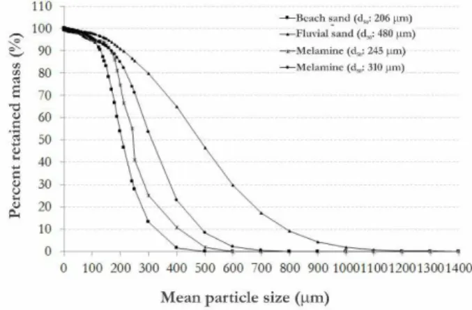
performed in three types of beds identiied as beach sand, river sand, and melamine, with density (ρS) and characteristic grain sizes
(d10, d50, d90, and d50*), which are shown in Table 1 and Figure 2. The dimensionless median grain sizes (d50*) were calculated by
Equation 1.
1 3 3 S
50 amb *
50 2
1 gd d
ρ −
ρ
=
ν
(1)
where ρamb is the water density (considered as 998.2 kg m -3), ρ
S is
the density of the bed sediment (kg m-3), g is the gravitational
acceleration (m s-2), d
50 is the average grain size (m), and ν is the
kinematic viscosity (m2 s-1).
Regarding the morphoscopic properties, both sands were sub-rounded and with sphericity degree between moderate
and high. In turn, melamine showed angular roundness and low
sphericity (KRUMBEIN, 1963).
After some tests, a good part of the iner fraction of
melamine had been transported to the output region of the acrylic
lume. For this reason, a new sampling and particle size analysis
of the melamine was performed, resulting in an average grain size of d50: 310 μm (named melamine 2).
Grains of the three types of material used in the mobile bed
were classiied according to Folk and Ward (1957) as moderately
selected, with selection degrees (σ (Φ)) (Equations 2 and 3) between 0.53 and 0.73.
%84 %16 %95 %5 ( ) :
4 6, 6
− −
σ Φ ×
(2)
being,
( )
2
: log d
Φ − (3)
where σ(Φ) is the degree of sediment selection in relation to the i parameter (Φ), Φ is the scaling parameter,% 84 is the 84th percentile of the sample,% 16 is the 16th percentile of the sample,% 95 is the 95th percentile of the sample,% 5 is the 5th percentile of the sample, and d is the particle size (μm).
In all, 29 tests were performed using three types of bed
material, two input discharges, three values of input mixture
concentration, and two lume slopes. Tests were named according to parameters, starting with the slope values (0.5º or 1.5º), followed
by the type of bed (melamine - M, beach sand - P, and river
sand - F), low (q - low lows and Q - high lows), and density
(low - 1, medium - 2, and high - 3). Tests with numbering 4 at the
end are related to repetitions performed with parameters similar
to those of inal 3.
The saline mixture was prepared in a reservoir of 5000 L capacity
(Figure 1a), with density values of 1015, 1025, and 1040 kg m-3
and respective salt concentrations of 26, 42, and 67 g L-1. After the
mixture homogenization, its temperature was measured with a thermometer and its density through a hydrometer After leveling
of the mobile bed, the approximate thickness of 5 cm, and slow illing of the lume with water (besides recording the temperature and density considered equal to 998.2 kg m-3), the experiment was
started. From the start of the pump (Figure 1b), the saline mixture
was introduced into the experimental lume (Figure 1d), being its
inlow recorded by the low meter (Figure 1c) coupled to the pipe. During the entire flow of the density current (Figure 3 - stained with a red dye for better visualization), the average velocity (Figure 1g - Ultrasound Velocity Proile - Duo
MetFlow AS) and concentration proiles (Figure 1h - siphons and
refractometer) were recorded throughout the experiment. Velocity proiles were composed of ten sensors (Figure 4a) disposed at
0.08, 2.15, 4.95, 7.9, 10.8, 13.7, 18, 22.4, 26.7, and 31.1 cm from the
mobile bed and positioned at 14 m of the saline stream injection,
with an acquisition frequency of 2 Hz. Proiles of average values
of concentration (Figure 4b) were constructed from samples
collected in 3.5 and 6 mm siphons of internal and external diameter, respectively, located at 2, 5, 10, 13, 18, and 21 cm of
Table 1. Grain size data of sediments used as mobile bed. Bed (kg mρ -3)
d10 d50 d90 d50*
(μm)
Melamine 1500 165 245 410 3.9
Melamine 2 1500 169 310 487 4.9
Sand beach 2600 131 206 324 4.8
River sand 2600 208 480 790 11.3
Figure 2. Grain size distribution of sediments used in mobile beds.
Figure 3. Density current performed in experiment 0.5Mq1* (Q: 380 L min 1, ρ
CD: 1016 kg m -3, C
the mobile bed and 15.5 m of the saline stream. Seven samples
were taken throughout the test, whose densities were read by a
portable refractometer ATAGO S28E 2 ~ 28% and converted
to salt concentration from a calibration curve performed in
laboratory (Equation 4)
0.643C 998.2
ρ = + (4)
where ρ is the saline density read by the refractometer (kg m- 3)
and C is the salt concentration (g L-1).
Furthermore, the analysis of the generation and development of bedforms as well as the current thickness was performed every
second based on pictures obtained laterally to the lume, using a Nikon D5000 camera (Figure 1f) as described by Koller (2016).
The output valve (sphere) located at the end of the masonry
lume (near its bottom and after 3 m of the end of acrylic lume)
was opened in order to keep the water level of the long tank (Figure 1i) shortly after the beginning of the experiment.
Finally, after pumping an average of 4000 L of the mixture per test (for about 8 min), the tank was slowly emptied in order to not disturb any bedforms generated by the density current.
After the full drainage of the long tank, pictures were
taken from the top along the whole acrylic lume.
Data analysis
During the low of density currents, characteristic velocity proiles (u) and concentration (c) are developed, whose vertical
values vary according to the distance in relation to the bed (z) and over time (t).
The calculation of average values of velocity (U), concentration (CCD), and thickness (H) of density currents in the
low direction was performed by summation of adapted Ellison
and Turner (1959) in Equations 5, 6, and 7.
( )
m 1 i i 1
i 1 i 0
i 1
u u
UH udz z z
2 − ∞ + + = +
=∫ = ∑ − (5)
( )
2 2 m 1
2 2 i i 1
i 1 i i 1
0
u u
U H u dz z z
2 ∞ − + + = +
=∫ = ∑ − (6)
( )
m 1
i i i 1 i 1
DC i 1 i
i 1 0
u c u c
UC H ucdz z z
2 ∞ − + + + = +
=∫ = ∑ − (7)
where U is the mean velocity of the density current (m s- 1), u is
the current velocity in the low direction (ms-1), H is the mean
current thickness (m), z is the vertical distance to the bed (m), CDC is the mean current concentration (g L-1), and c is the current
concentration at the sampling point (g L- 1).
Near-bed shear velocities (u*) were estimated based on velocity data collected near the mobile bed-current density interface, in the region below the maximum current velocities. This region
of the velocity proile presented a logarithmic distribution for
all tests of the present work and, therefore, the shear velocity
calculation of the low was performed according to Equation 8 as
already applied for current density, according to Altinakar, Graf
and Hopfinger (1996) and Manica (2009).
* 0
u 1 z ln
u z
=
κ (8)
where u is the current velocity in low direction (m s- 1), z is the
distance to the bed (m), z0 is the distance to the point where the velocity reaches zero (m), u* is the shear velocity (ms-1), and κ is
the von Kármán constant (0.41).
The shear velocity represents an intensity measure of the
turbulent luctuations (GRAF, 1971) and is used on the shear
stress calculation of the low near the bed (τb) which, in turn, is an input parameter in phase diagrams from Simons and Richardson (1961). Such calculation was based on Equation 9 adapted from
luvial lows (YALIN, 1972), replacing the density of luvial low by density currents (ρCD), neglecting any stresses from the luid.
b *
DC
u = τ
ρ (9)
where u* is the shear velocity (m s-1), τ
b is the shear stress near the
bed (N m-2), and ρ
DC is the density of the density current (kg m -3).
Finally, the calculation of the grain mobility parameter (θ) and
the dimensionless median grain size (d50*) used as input parameters
of the Van den Berg and Van Gelder diagram (VAN DEN BERG; VAN GELDER, 1993) are presented in Equations 10 and 11.
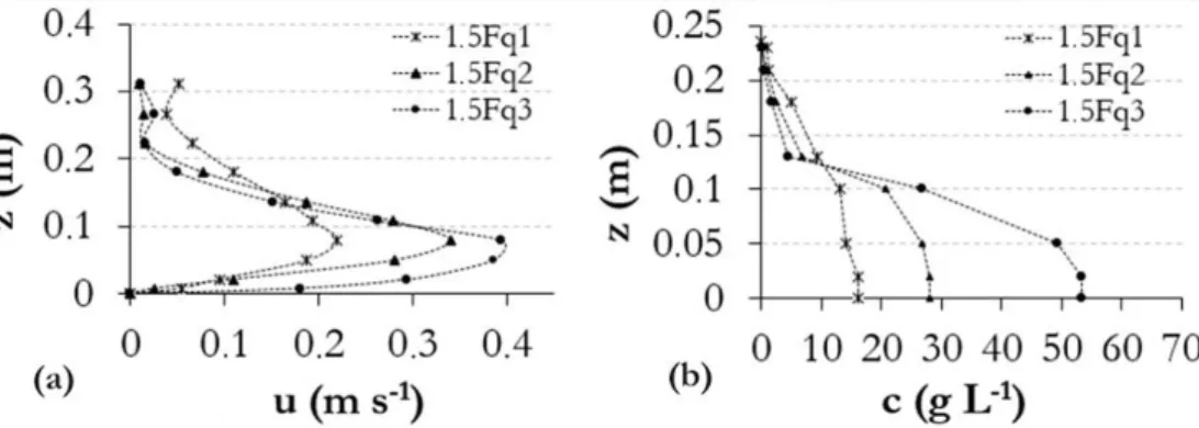
Figure 4. Velocity (a) and concentration (b) proiles of density currents from experiments 1.5Fq1 (U= 0.15 m s-1 and C
CD=9.0 g L -1),
1.5Fq2 (U= 0.24 m s-1 and C
CD= 16.3 g L
-1) and 1.5Fq3 (U= 0.29 m s-1 and C
( )
2 DC
2
S DC 50
U '
C ' d
ρ θ =
ρ − ρ (10)
being,
90
4H C ' 18 log
d
=
(11)
where, θ’ is the grain mobility parameter, ρDC is the density of the density current (kg m-3), ρ
S is the density of the bed sediment
(kg m- 3), U is the current mean velocity (m s-1), H is the current
mean thickness (m), C’ is the Chézy’s coeficient, d50 is the mean grain size (m), d90 is the characteristic grain size, in which 90% of particles show smaller sizes (m) and d50 is the median grain size (m).
The relation between the inertial and gravitational forces
of density currents deined by the dimensionless densimetric
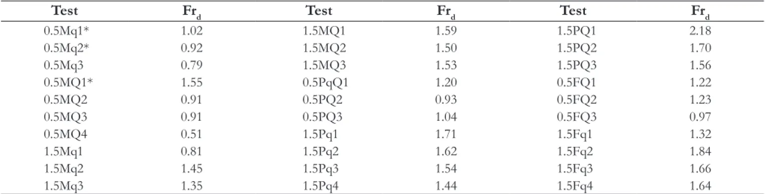
Froude (Frd) classiies it in subcritical (Frd<1), critical (Frd=1), and supercritical (Frd>1) regimes, as shown in Equation 12.
d DC amb amb U Fr gH = ρ − ρ
ρ
(12)
where U is the average velocity of the density current (m s-1), ρ DC is
the density of the density current (kg m-3), ρ
amb is the density of the
ambient water (kg m-3), g is the gravitational acceleration (m s- 2),
and H is the current mean thickness (m).
The parameter presented above, together with the dimensionless relationship between the hydraulic radius (Rh) and d50 (deined by
the author as relative submergence) presented in Equation 13 are used in the Athaullah’s phase diagram (1968 apud JULIEN, 1998).
h
A lh R
p l 2h
= =
+ (13)
where l and h are considered the width and the thickness of the
low, respectively. For the calculation of this parameter, the present
study considered the stream average height and the width of the
two-dimensional lume.
Besides parameters related to currents and mobile beds used in the diagram analysis, it was also necessary to know the types
of generated bedforms. Thus, the bedforms were classiied with
regard to two factors: (a) sediment transport near the bed and the
presence of suspended sediments during its generation, veriied
by images obtained during the tests and (b) the size of bedforms.
RESULTS
Density current
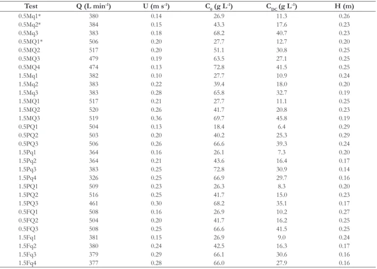
The average values of velocity and concentration of density currents obtained from their respective proiles and using
Equations 5 and 6 are presented in Table 2.
All velocity and concentration proiles follow classic
trends for density currents as stated by other authors (FABIAN, 2002; MANICA, 2009; SEQUEIROS, 2012; PUHL, 2012). Figure 4 shows velocity (Figure 4a) and concentration
proiles of density currents (Figure 4b) which were analyzed in the present study.
Velocity values are reduced near the bed due to the interaction between the low and the mobile bed and then increase up to a maximum point (positive velocity gradient), deining the lower boundary layer of the proile similar to a turbulent boundary
layer (YALIN, 1972).
As can be seen in Figure 4, this region was characterized by four sampling points (considering u* null at rate 0). Based on
these values and the use of Equation 8, the shear velocity of the low near the bed (u*) could be calculated (Table 3). Above the maximum velocity value, they keep decreasing until reach the upper stream layer (mixture layer), where there is greater incorporation
of the ambient water present in the long tank and consequent
decrease of concentration of the density current.
However, concentration proiles (Figure 4b) presented higher values near the bed, attenuating along the vertical until reach the interface with the ambient water, where there is a greater incorporation of the ambient water.
Shear stresses (τb), fundamental in the deinition of
forces exerted by the low and used in the calculation of the
mobility parameter of the Simons and Richardson diagram (SIMONS; RICHARDSON, 1961), were calculated from
Equations 8 and 9 and are presented in table 3.
Shear velocities (u*) for all the tests ranged from 0.08 to 2.51 m s- 1 and
the shear stress (τb) between 0.18 and 3.25 N m -2.
Table 4 shows mobility parameters (θ’) calculated from
Equations 10 and 11 with values ranging from 0.01 to 0.33. The maximum values of θ’ occur for beds composed of melamine and for high discharge lows, concentrations and lume slopes, indicating the high mobility of this sediment for
the referred hydraulic conditions.
On the other hand, the lower values of θ’ resulting from
experiments performed on river sand (of greater diameter and density than melamine), pointing to this sediment as the most
dificult to be mobilized.
The densimetric Froude number contemplated a
considerable range of values (between 0.5 and 2.2) (Table 5),
occurring 8 experiments with low of subcritical regime and 21 in
the supercritical regime, as shown in Table 5.
In general, density currents with low Frd values have developed
plane beds and smaller bedforms, such as ripples. Inasmuch as
Frd increased, bedforms also increased in size (length and height), tending to generate dunes and/or supercritical plane beds.
Bedforms
Based on the lateral images obtained during the tests together with the calculated shear stress values, it was possible to classify the bedforms generated in lower plane bed, ripples, and dunes (Figure 5).
The lower plane bed occurred with high frequency,
Table 2. Discharge (Q), velocity (U), thickness (H) and concentrations of mixture (C0) and density current (CDC).
Test Q (L min-1) U (m s-1) C0 (g L-1) CDC (g L-1) H (m)
0.5Mq1* 380 0.14 26.9 11.3 0.26
0.5Mq2* 384 0.15 43.3 17.6 0.23
0.5Mq3 383 0.18 68.2 40.7 0.23
0.5MQ1* 506 0.20 27.7 12.7 0.20
0.5MQ2 517 0.20 51.1 30.8 0.25
0.5MQ3 479 0.19 63.5 27.1 0.25
0.5MQ4 474 0.13 72.8 41.5 0.25
1.5Mq1 382 0.10 27.7 10.9 0.24
1.5Mq2 383 0.22 39.4 18.0 0.20
1.5Mq3 383 0.28 65.8 32.7 0.19
1.5MQ1 517 0.21 27.7 11.1 0.25
1.5MQ2 520 0.26 41.7 20.8 0.23
1.5MQ3 519 0.36 69.7 45.8 0.19
0.5PQ1 504 0.13 18.4 6.4 0.29
0.5PQ2 503 0.20 40.2 25.3 0.29
0.5PQ3 506 0.26 66.6 39.3 0.24
1.5Pq1 364 0.16 26.1 7.3 0.20
1.5Pq2 364 0.21 43.6 16.4 0.17
1.5Pq3 383 0.25 72.8 30.9 0.14
1.5Pq4 326 0.25 66.9 29.7 0.16
1.5PQ1 509 0.23 26.3 8.3 0.20
1.5PQ2 516 0.25 41.7 15.0 0.23
1.5PQ3 461 0.30 68.2 35.1 0.17
0.5FQ1 508 0.16 26.9 10.2 0.27
0.5FQ2 504 0.20 41.7 16.2 0.25
0.5FQ3 508 0.25 66.6 41.5 0.25
1.5Fq1 381 0.15 26.9 9.0 0.24
1.5Fq2 380 0.24 42.5 16.3 0.17
1.5Fq3 379 0.29 66.1 30.6 0.16
1.5Fq4 377 0.28 66.0 27.9 0.16
* Experiments performed with the “melamine 2” sediment. Table 3. Calculated velocity s (u*) and shear (τb) stresses.
Test (m su*-1) (N mτb -2) Test (m su*-1) (N mτb-2)
0.5Mq1* 0.14 0.21 0.5PQ3 0.49 1.60
0.5Mq2* 0.29 0.44 1.5Pq1 0.08 0.26
0.5Mq3 0.61 0.69 1.5Pq2 0.32 1.06
0.5MQ1* 1.13 1.70 1.5Pq3 0.20 0.66
0.5MQ2 0.22 0.25 1.5Pq4 0.22 0.73
0.5MQ3 0.37 0.43 1.5PQ1 0.50 1.66
0.5MQ4 0.28 0.32 1.5PQ2 0.23 0.78
1.5Mq1 0.15 0.18 1.5PQ3 0.44 1.46
1.5Mq2 0.92 1.08 0.5FQ1 0.22 1.69
1.5Mq3 2.51 2.90 0.5FQ2 0.09 0.71
1.5MQ1 0.42 0.49 0.5FQ3 0.10 0.74
1.5MQ2 1.27 1.50 1.5Fq1 0.11 0.88
1.5MQ3 1.43 1.62 1.5Fq2 0.42 3.25
0.5PQ1 0.10 0.32 1.5Fq3 0.28 2.18
0.5PQ2 0.19 0.64 1.5Fq4 0.33 2.55
* Experiments performed with the “melamine 2” sediment.
The beginning of ripples generation occurred in a slow way, where the interaction between the low and the bed did not allow the suspension of large amounts of sediment, perceptible by the image analyses. These bedforms presented mild upstream slopes and more abrupt downstream slopes occurring in 13 of the 29 experiments.
Dunes were identiied in four tests within 29 performed (1.5Mq2, 1.5Mq3, 1.5MQ2, and 1.5MQ3). These bedforms
differ from ripples due to the high shear stress applied by
the low near the bed (1.08 < τb (N m
-2) < 2.90) and by the
Table 4. Chézy’s coeficient values (C’) and the mobility parameter (θ’).
Test C’ θ’ Test C’ θ’
0.5Mq1* 60.0 0.04 0.5PQ3 62.6 0.05
0.5Mq2* 60.3 0.04 1.5Pq1 60.9 0.02
0.5Mq3 60.2 0.08 1.5Pq2 59.7 0.04
0.5MQ1* 58.0 0.08 1.5Pq3 58.2 0.06
0.5MQ2 61.0 0.09 1.5Pq4 59.1 0.05
0.5MQ3 60.8 0.08 1.5PQ1 61.2 0.04
0.5MQ4 60.9 0.04 1.5PQ2 62.0 0.05
1.5Mq1 60.5 0.02 1.5PQ3 59.7 0.08
1.5Mq2 59.1 0.11 0.5FQ1 56.3 0.01
1.5Mq3 58.7 0.20 0.5FQ2 56.1 0.02
1.5MQ1 61.1 0.10 0.5FQ3 55.7 0.03
1.5MQ2 60.4 0.16 1.5Fq1 55.4 0.01
1.5MQ3 58.9 0.33 1.5Fq2 52.6 0.03
0.5PqQ1 63.9 0.01 1.5Fq3 52.4 0.04
0.5PQ2 63.8 0.03 1.5Fq4 52.4 0.04
* Experiments performed with the “melamine 2” sediment.
Table 5. Values of densimetric Froude number (Frd) of the experimentally generated density currents.
Test Frd Test Frd Test Frd
0.5Mq1* 1.02 1.5MQ1 1.59 1.5PQ1 2.18
0.5Mq2* 0.92 1.5MQ2 1.50 1.5PQ2 1.70
0.5Mq3 0.79 1.5MQ3 1.53 1.5PQ3 1.56
0.5MQ1* 1.55 0.5PqQ1 1.20 0.5FQ1 1.22
0.5MQ2 0.91 0.5PQ2 0.93 0.5FQ2 1.23
0.5MQ3 0.91 0.5PQ3 1.04 0.5FQ3 0.97
0.5MQ4 0.51 1.5Pq1 1.71 1.5Fq1 1.32
1.5Mq1 0.81 1.5Pq2 1.62 1.5Fq2 1.84
1.5Mq2 1.45 1.5Pq3 1.54 1.5Fq3 1.66
1.5Mq3 1.35 1.5Pq4 1.44 1.5Fq4 1.64
* Experiments performed with the “melamine 2” sediment.
Figure 5. Bedforms generated. (a) lower plane bed, (b) ripples, and (c) dunes.
Phase diagrams
Based on presented hydraulic parameters together with types of generated bedforms, the input parameters of phase diagrams were calculated and are presented below.
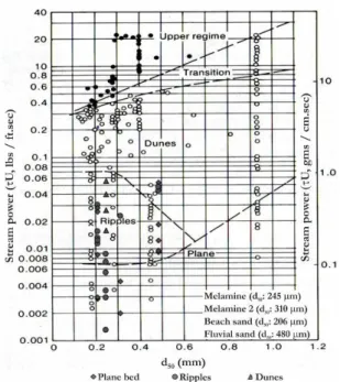
Simons and Richardson (1961)
This phase diagram was a pioneer in the attempt to predict the bedform types, seeking to relate data from average grain size (d50) with low’s energy (Uτ). Figure 6 shows these parameters for tested density currents in the Simons and Richardson diagram, indicating the incidence of most points in the prediction region of ripples.
Only three points were found in the dune prediction referring
to 1.5Fq2, 1.5Fq3, and 1.5Fq4 tests, conducted in sand-bed river
(d50 = 480 μm), whereas the last two showed ripples with high wavelengths.
Besides ripples, it can be observed the occurrence of
Figure 6. Experimental results applied to the Simons and Richardson diagram (SIMONS; RICHARDSON, 1961).
triangles) and seven lower plane beds (1.5Fq1, 0.5FQ3, 0.5FQ2, and 0.5FQ1 - river sand and 0.5Pq2, 0.5Pq3, and 1.5PQ1 - beach
sand). Even in the ripple region, it is emphasized the proximity
of the 1.5Mq3 experiment (with larger dimensions) with the self-prediction region showed coherence in the low’s energy and the average grain size required to generate this bedform.
Experiments whose points are located in the predicted region to form lower plane bed resulted in ripples
(0.5Mq2, 0.5MQ3, 0.5MQ4, and 1.5Mq1) and lower plane beds (0.5Mq1*, 0.5Mq2*, 0.5Pq1, and 1.5Pq1). The occurrence of
ripples in this region can be explained by the composition of the bed used in these tests (melamine), which has been shown to be an easier material to be remobilized due to its low density.
Although melamine has a density of 1500 kg m- 3 (plastic material),
the sand has approximately 2650 kg m-3 due to its quartz composition.
Finally, the diagram showed good predictions for ripples generated in beds composed of beach sand, similar sediment to
that used by the diagram’s author.
Southard and Boguchwal (1990)
Average velocities of density currents, together with the average grain size of the tested bedforms in the Southard and Boguchwal diagram (SOUTHARD; BOGUCHWAL, 1990) are shown in Figure 7.
Although the present study identiied three distinct bedforms
(lower plane bed, ripples, and dunes), these authors predicted only the generation of ripples based on average velocities of density currents and the average grain size of the used bedforms.
As a hypothesis of differences between the observed bedforms and those predicted by the diagram, the bedform from
velocity proiles of the luvial lows (from which the diagram
was elaborated) is emphasized, which is different from density
currents. This might have inluenced both the calculated average
stream velocity (y-axis of the diagram) and the velocity near the bed. Furthermore, the average grain size (parameter used on the x-axis of the diagram) does not consider the density of the material present in the bed, which impairs its comparison with studies performed with different sediments.
Additionally, the cited differences relate to test conditions
used by the author, who established average low thicknesses between 0.25 and 0.40 m and used only sand as mobile bed material.
Athaullah (1968 apud JULIEN, 1998)
This author constructed a classiication diagram for bedforms, considering the low regime (subcritical, critical, and
supercritical) by calculating the dimensionless Froude numbers (Fr) and by the relationship between the hydraulic radius (Rh) and the average grain size (d50) - deined as relative submergence.
Although Froude number deined low regimes through their values (smaller, equal or greater than unity), Athalluah
(1968 apud JULIEN, 1998) constructed his diagram deining these regimes based on the occurrence of ripples and dunes (Supercritical regime), plane bed transition (critical regime), and antidunes, falls, and pools (supercritical regime). The uncertainty associated with the direct use of the Froude number for the prediction of bedforms is emphasized by the authors.
Figure 7. Experimental results plotted in the Southard and Boguchwal diagram (SOUTHARD; BOGUCHWAL, 1990).
In the present study, the use of this diagram was adapted by
calculating the densimetric Froude number (Frd), which considers the small density difference between the current and the ambient
luid in the thrust force.
Figure 8 shows Frd values and relative submergence (Rh/d50)
calculated for the experimental current densities. It was identiied the
simultaneous occurrence of the three types of generated bedforms
(plane bed, ripples, and dunes) in a region deined by approximate
values of Frd=1.5 and Rh/d50= 3000. In other words, with the exception
of the test 0.5MQ4 (Q= 474 L min-1, U= 0.13 ms-1, and Fr d=0.5),
all plotted points were restricted to the region of the predicted
low chart of supercritical regime (even with Frd smaller than 1)
and of antidunes’ formation. However, none of the bedforms
generated by density currents showed antidune characteristics (very symmetrical forms, larger dimensions in relation to the
dunes, and low surface in phase with bedforms, according to
Simon and Richardson (1961) and Engelund and Fredsϕe (1982)). Furthermore, there are plane beds and ripples mapped in regions with high Frd, however, these forms were not predicted
for supercritical luvial low regimes.
Although they differ from results found by Athaullah, the values of the present study approximate those found by Puhl (2012), showing consistency among the observations of bedforms by density currents.
Finally, the dimensionlessness of results in the mentioned parameters does not show any evident trend for grouping on the regions in the diagram, precluding its use for the prediction of bedforms by density currents. The use of Frd might have inluenced this result, since the density difference between the current and the
ambient luid must be considered in this calculation (differently
from the Fr number).
The wide use of the Froude number (Fr) in the classiication of bedforms generated by luvial low is highlighted. However,
several studies (FEDELE; GUENTZEL; HOYAL, 2009; PUHL, 2012; CARTIGNY; POSTMA, 2016) show the need for adapting the prediction of bedforms generated by density currents based on Frd, since the proiles of velocity and concentration and hence
the hydraulic processes present in these lows differ from those
to the free surface.
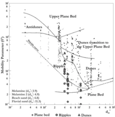
Van den Berg and Van Gelder (1993)
This diagram is a review of Van Rijn’s diagram (VAN RIJN, 1984),
which considers the inluence of shear stresses on the occurrence
and dimensions of bedforms as a basic element of this approach and relates the average dimensionless grain size (d50*) with the
mobility parameter (θ’).
Figure 9 shows the application of these parameters to the tested density currents and to the used bedforms.
All experiments that generated ripples (indicated by circles) are located in the region predicted for this type of bedform regardless of the type and average grain size of sediment used in the mobile bed (melamine or sand).
Among the four experiments classiied as dunes, only 1.5MQ3 is located in the prediction region for these bedforms due to the
inluence of its high velocity in the calculation of mobility parameter. The other three experiments (1.5Mq2, 1.5Mq3, and 1.5MQ2),
although located in the prediction region of ripples, are close to the region established for dunes, according to the author.
It should be noted that the lower region of the diagram
predicts the occurrence of lower plane bed, where four from
the twelve experiments showed this coniguration. Although the
rest of the generated lower plane beds (indicated by diamonds) have been located in the prediction region of ripples, they are still below the Shields curve (region of absence of particle movement, according to Shields (1936)).
Thus, the results obtained in the present study seem to
correspond well with those predicted by Van den Berg and Van
Gelder diagram (VAN DEN BERG; VAN GELDER, 1993). This is because these authors have correlated dimensionless parameters in their prediction, allowing the comparison of results obtained with different scales and sediment compositions.
CONCLUSIONS
The present study generated three types of bedforms (lower plane bed, ripples, and dunes) through experiments with
density currents, on a reduced scale. The parameters’ analysis
of these currents and sediments used in the composition of the mobile beds made it possible to calculate the input parameters
of three types of prediction diagram of luvial bedforms besides the veriication of their application and validity in the prediction
of bedforms by density currents.
Results showed that bedforms generated by density currents presented disagreements in relation to those predicted by
the discussed luvial stability diagrams. Regarding dimensionless
diagrams of Simons and Richardson (1961) and Southard and Boguchwal (1990), this disagreement may have been inluenced by the difference between the materials (size, density, shape) used in the present study in relation to those used in the cited diagrams.
Athaullah’s diagram (1968 apud JULIEN, 1998) despite using dimensionless parameters in its analysis, clearly did not show a
good correlation with observations of luvial lows neither grouped the different bedforms. However, Van den Berg and Van Gelder
(1993) grouped the data in different regions, although they did
not respect the prediction limits of luvial bedforms.
The hydraulic differences between the luvial lows (free
surface) when compared to the density currents (two different
interfaces and different velocity and concentration proiles) are
highlighted as the main source of the differences between the experimental results of this study and the presented phase diagrams
Thereby, it is evident the need for speciic studies that
help in the elaboration of a proper diagram for the prediction of bedforms generated by density currents. Such a diagram can only be obtained from observations under experimentally controlled conditions, through safety in the correlation of hydrodynamic and sedimentological data.
ACKNOWLEDGEMENTS
The irst author acknowledges CNPq (National Council for Scientiic and Technological Development) and, together with the
other authors, to the ExxonMobil Upstream Research Company.
REFERENCES
ALTINAKAR, M. S.; GRAF, W. H.; HOPFINGER, E. J. Flow structure in turbidity currents. Journal of Hydraulic Research, v. 34, n. 5, p. 713-718, 1996. http://dx.doi.org/10.1080/00221689609498467.
CARTIGNY, M. J. B.; POSTMA, G. Turbidity current bedforms.
In: GUILLEN, J.; ACOSTA, J.; CHIOCCI, F. L.; PALANQUES, A.
Atlas of bedforms in the Western Mediterranean. New York: Springer, 2016. p. 29-33.
CHANG, H. H. Fluvial processes in river engineering. New York: John Wiley, 1988. p. 432.
ELLISON, T. H.; TURNER, J. S. Turbulent entrainment in stratified flows. Journal of Fluid Mechanics, v. 6, n. 3, p. 423-448, 1959. http://
dx.doi.org/10.1017/S0022112059000738.
ENGELUND, F.; FREDSΦE, J. Sediment ripples and Dunes. Annual Review of Fluid Mechanics, v. 14, n. 1, p. 13-37, 1982. http://
dx.doi.org/10.1146/annurev.fl.14.010182.000305.
FABIAN, S. Modelagem física de correntes de densidade conservativas em canal de declividade variável. 2002. 107 f. Dissertação (Mestrado em
Engenharia) - Instituto de Pesquisas Hidráulicas. Programa de Pós-Graduação em Engenharia de Recursos Hídricos e Saneamento
Ambiental, Universidade Federal do Rio Grande do Sul, Porto Alegre, 2002.
FEDELE, J. J.; GUENTZEL, K.; HOYAL, D. C. Experiments
on bedforms created by density currents. In: RIVER, COASTAL AND ESTUARINE MORPHODYNAMICS SYMPOSIUM, 9.,
2009, Boca Raton. Proceedings... Boca Raton: CRC Press, 2009. p. 833-840.
FEDELE, J. J.; HOYAL, D. C.; DRAPER, J. M. Supercritical
bedforms under density currents. In: RIVER COASTAL AND ESTUARINE MORPHODYNAMICS – RCEM, 5., 2011, Beijing,
China. Proceedings... Beijing: Regional Civil Society Engagement Mechanism, 2011. p. 1- 9.
FOLK, R. L.; WARD, W. C. Brazos River bar: a study in the significance of gran size parameters. Journal of Sedimentary Petrology,
v. 27, n. 1, p. 3-26, 1957.
http://dx.doi.org/10.1306/74D70646-2B21-11D7-8648000102C1865D.
GRAF, W. H. Hydraulics of sediment transport. New York:
McGraw-Hill, 1971. 513 p. (Series in Water Resources and Environmental
Engineering).
HAND, B. M. Supercritical flow in density currents.Journal of Sedimentary Petrology, v. 44, n. 3, p. 637-648, 1974.
JULIEN, P. Y. Erosion and sedimentation. Cambridge: Cambridge University Press, 1998.
KNELLER, B. C.; BENNETT, S. J.; MCCAFFREY, W. D. Velocity and turbulence structure of density currents and internal solitary waves: potential sediment transport and the formation of wave ripples in deep water. Sedimentary Geology, Amsterdam, v. 112, n. 3-4, p.
235-250, 1997. http://dx.doi.org/10.1016/S0037-0738(97)00031-6.
KOLLER, D. K. Estudo experimental de formas de fundo por correntes de densidade salina em canal de fundo móvel. 2016. 120 f. Dissertação
(Mestrado em Recursos Hídricos e Saneamento Ambiental) - Instituto de Pesquisas Hidráulicas, Universidade Federal do Rio
Grande do Sul, Porto Alegre, 2016.
KRUMBEIN, W. C. Stratigraphy and sedimentation. 2nd ed. San Francisco: Freeman, 1963. 660 p.
MANICA, R. Geração de correntes de turbidez de alta densidade: condicionantes hidráulicos e deposicionais. 2009. 391 f. Tese (Doutorado
em Recursos Hídricos e Saneamento Ambiental) - Instituto de Pesquisas Hidráulicas, Universidade Federal do Rio Grande do
Sul, Porto Alegre, 2009.
MIDDLETON, G. V. Experiments on density and turbidity currents I. Motion of the head. Canadian Hournal of Earth Sciences,
v. 3, n. 4, p. 523-546, 1966. http://dx.doi.org/10.1139/e66-038.
MIDDLETON, G. V. Sediment deposition from turbidity currents.
Annual Review of Earth Planet Science, v. 21, p. 89-114, 1993.
PARKER, G.; GARCIA, M.; FUKUSHIMA, Y.; YU, W. Experiments on turbidity currents over an erodible bed. Journal of Hydraulic Research, v. 25, n. 1, p. 123-147, 1987. http://dx.doi. org/10.1080/00221688709499292.
PUHL, E. Morfodinâmica e condição de equilíbrio do leito sob a ação de correntes de turbidez. 2012. 155 f. Tese (Doutorado em Recursos
Hidráulicas, Universidade Federal do Rio Grande do Sul, Porto
Alegre, 2012.
RAUDKIVI, A. J. Loose boundary hydraulics. 3rd ed. Oxford:
Pergamon Press, 1990. 538 p.
RAUDKIVI, A. J. Ripples on stream bed. Journal of Hydraulic Engineering, v. 123, n. 1, p. 58-64, 1997. http://dx.doi.org/10.1061/
(ASCE)0733-9429(1997)123:1(58).
SEQUEIROS, O. E. Estimating turbidity current conditions from channel morphology: a Froude number approach.Journal of Geophysical Research, v. 117, n. 4, p. 1-17, 2012. http://dx.doi.
org/10.1029/2011JC007201.
SHIELDS, A. Anwendung der Aehnlichkeitsmechanik und der Turbelens Forschung auf die Geschiebebewegung. Berlim: Mitteeilungen der
Preussische Versuchanstalt für Wasserbau und Schiffbau, 1936.
SIMONS, D. B.; RICHARDSON, E. V. Forms of bed roughness in alluvial channels. Journal of the Hydraulics Division, New York, v.
87, n. 3, p. 87-105, 1961.
SIMPSON, E. J. Gravity currents in the environment and the laboratory. 2nd ed. Cambridge: Cambridge University, 1997. 244 p.
SOUTHARD, J. B.; BOGUCHWAL, L. A. Bed configurations in steady unidirectional water flows: Part 2. Synthesis of flume data. Journal of Sedimentary Petrology, v. 60, n. 5, p. 658-679, 1990. http://
dx.doi.org/10.1306/212F9241-2B24-11D7-8648000102C1865D.
SPINEWINE, B.; SEQUEIROS, O. E.; GARCIA, M. H.; BEAUBOUEF, R. T.; SUN, T.; SAVOYE, B.; PARKER, G. Experiments on wedge-shaped deep sea sedimentary deposits in mini basins and/or on channel levees emplaced by turbidity
currents. Part II. Morphodynamic evolution of the wedge and
of the associated bedforms. Journal of Sedimentary Research, v. 79, n. 8, p. 608-628, 2009. http://dx.doi.org/10.2110/jsr.2009.065.
VAN DEN BERG, J. H.; VAN GELDER, A. 1993. A new bedform stability diagram, with emphasis on the transition of
ripples to plane bed in flows over fine sand and silt. In: MARZO, M.; PUIGDEFÁBREGAS, C. (Ed.). Alluvial sedimentation. Boston: Blackwell, 1993. p. 11-21.
VAN RIJN, L. C. Sediment transport, part III: bed forms and
alluvial roughness. Journal of Hydraulic Engineering, v. 110, n. 12,
p. 1733-1754, 1984. http://dx.doi.org/10.1061/(ASCE)0733-9429(1984)110:12(1733).
WINTERWERP, J. C.; BAKKER, W. T.; MASTBERGEN, D. R.; VAN ROSSUM, H. Hyperconcentrated sand-water mixture
flows over erodible bed. Journal Hydraulic Engineering, v. 118,
p. 1508-1525, 1992.
YALIN, M. S. Mechanics of sediment transport. Nova York: Pergamon Press, 1972.
Authors Contributions
Débora Karine Koller: achievement of research, experiment’s
survey and data processing, research design and manuscript writing.
Ana Luiza de Oliveira Borges: research design, contribution and correction of the manuscript.
Eduardo Puhl: research design, contribution and correction of the manuscript.