Three Applications of the
Marginal Cost of Public Funds Concept
Bev Dahlby
Department of Economics
University of Alberta
Edmonton Alberta
Canada, T6G 2H4
[email protected]
(April 2005)
Abstract
This paper illustrates the use of the marginal cost of public funds concept in three
This paper illustrates the use of the marginal cost of public funds (MCF) concept
in three contexts:
• the computation of the MCFs for excise taxes in the United Kingdom;
• the computation of the MCF for payroll taxes in a labour market with involuntary
unemployment
• the derivation and computation of an optimal flat tax.
In the first application, we extend the recent paper by Parry (2003) by (a)
distinguishing between consumption externalities (e.g. second-hand smoke from
cigarettes) and public expenditure externalities (e.g. the increase in public health care
costs caused by smoking), (b) incorporating the distortions caused by imperfect
competition in the cigarette market, and (c) distinguishing between the MCFs for per unit
and ad valorem taxes on cigarettes. Our base case calculations indicate that the MCFs for
taxes on petrol and alcohol are 3.00 and 1.42 respectively. Incorporating the distortion
caused by market power increases the MCF for the excise taxes on cigarettes, but these
MCFs are still less than one and lower that the MCFs for the other excise taxes. The per
unit excise tax on cigarettes has an MCF of 0.978, while the ad valorem tax on cigarettes
is slightly higher at 0.981. These results contradict the standard result in the
literature―ad valorem taxes are superior to per unit excise taxes in an imperfectly
competitive market. The standard result is not necessarily valid when there are other
distortions in the market because under these conditions social welfare may be improved
by raising the price of the product, and a per unit tax is more effective in raising the price
of the product than an ad valorem tax.1
1
In the second application, we incorporate one of the most important labour market
distortions, involuntary unemployment, in the measurement of the MCF. The MCF from
taxing labour has been extensively studied.2 However, none of the studies incorporates
the distortion created by the involuntary unemployment in the calculation of the MCF.
We use the Shapiro and Stiglitz (1982) efficiency wage model as a framework for
modeling the effect of taxes on level of unemployment. Our analysis shows, using
numerical values based on the Canadian labour market, that incorporating involuntary
unemployment significantly increases the MCF for an employer payroll tax by 25 to 50
percent.
In the third application, we analyze the optimal “flat tax”, which is an income tax
where all earnings above a given exemption level, X, are taxed a constant marginal tax
rate, m. The flat tax is a progressive tax because the average tax rate increases with the
taxpayer’s income if they earn more than the basic exemption level. The flat tax can be
made more progressive, for a given tax yield, by increasing X and m. One reason for
focusing on the flat tax is that it has been advocated by tax reformers such as Hall and
Rabushka (1995) in the United States, and the flat tax has been adopted by the province
of Alberta. However, the basic analytics of an optimal flat tax have not been fully
articulated in the literature. In this section, we derive expressions for the
distributionally-weighted marginal cost of funds from increasing the basic exemption level, SMCFX, and
for an increase in the marginal tax rate, SMCFm. The optimal flat tax is characterized by
the condition that SMCFX = SMCFm , and we use this condition to provide some insights
into the structure of an optimal flat tax. However, like most optimal income tax
2
problems, the optimality conditions are sufficiently complex that we need to simulate the
model in order to fully appreciate their implications. We use the model to compute the
optimal flat tax for a government that needs to raise the same revenues as a 20 percent
proportional tax on earnings. Our computations indicate that the optimal exemption level
would be relatively high (43 percent of earners would not pay the tax) and the optimal
marginal tax rate would be over 40 percent even with relatively modest distributional
objectives. It is hoped that future research will show how this approach can be
generalized and used to evaluate multi-bracket optimal tax systems.
1.0 The MCFs for Excise Taxes in the U.K.
In a recent paper, Parry (2003) calculated the marginal excess burdens for excise
taxes on petrol, alcoholic beverages, and cigarettes in the United Kingdom. In this
section, we use Parry’s benchmark parameter values and extend his analysis of the
efficiency effects of excise taxation by:
• including commodity taxes on all other goods,
• distinguishing between consumption and public expenditure externalities,
• incorporating the distortions caused by imperfect competition in the cigarette
market
• distinguishing between the MCFs for per unit and ad valorem taxes on cigarettes.
Our calculations are primarily meant to illustrate how these various factors can be
incorporated in the calculation of the MCFs for excise taxes. Perhaps the most
by imperfect competition in the cigarette industry in calculating the MCF from cigarette
taxes.
The MCFs for the excise taxes are calculated in the context of a model where a
representative individual allocates his expenditures among four commodities, the xjs, and
his time between work and leisure. We will define commodity 1 as petrol, commodity 2
as alcoholic beverages, commodity 3 as tobacco products, and commodity 4 as all other
goods. His budget constraint is:
(
)
∑
=
τ − =
4
1 j
w j
jx 1 wL
q (1)
where qj is the consumer price of commodity j, the after-tax wage rate is (1 - $w)w, and L
is amount of labour supplied. Since L = T – x0, where x0 is the individual’s leisure time
and T is total amount of time available for work or leisure, the budget constraint can also
be written in the following form:
∑
=
=
4
0 j
0 j jx q T
q (2)
where q0 = (1 - $w)w is the “price” of leisure, and q0T is the individual’s total potential
net earnings. Total tax revenues are equal to:
∑
∑
∑
∑
= π =
= =
πΠ = τ + τ + τ Π
τ + τ + τ
=
4
1 j
j j 4
0 j
w j j j 4
1 j
4
1 j
j j w
j j
jq x wL q x wT
R (3)
where
j
π
τ is the tax rate on profit earned in the jth market, j. The effective tax rate on
leisure, $0 = -$w/(1 - $w), is negative, reflecting the fact that wage taxes reduce the
opportunity cost of leisure.
The MCFs depend on the price sensitivity of the tax bases; the distortions in each
between tax bases based on their substitutability or complementarity. All of these
elements are incorporated in the following formula for the MCF for a tax on commodity
i:
(
)
(
(
)
)
(
)
∑
(
)
∑
= π π π = π π π ε δ − δ τ + τ + τ + τ − ε δ τ − + δ − τ + τ − = 4 0 j i i ji G M j j i i i i 4 0 j i i ji M E j i i i i t dt dq b dt dq b 1 b dt dq 1 b dt dq b 1 b MCF j j j i j j j j i ii (4)
where:
bi is the budget share of commodity i, qixi/q0T;
j E
δ is the distortion in the market for commodity j caused by environmental externalities;
j M
δ is the distortion in the market for commodity j caused by imperfect competition;
j G
δ is the distortion in the market for commodity j caused by government expenditure
externalities;
ji is the (uncompensated) elasticity of demand for commodity j with respect to the price
of commodity i;
$j is the ad valorem (equivalent) tax rate on commodity j;
dqi/dti is the degree to which the per unit excise taxes, ti, are shifted to consumers.
In order to calculate the MCFs for the excise taxes on petrol, alcoholic beverages, and
cigarettes, we need values for the excise and profit tax rates, the budget shares of the
commodities, the own and cross-price elasticities of demand for each of the commodities,
the distortions caused by externalities and imperfect competition, and the degree of tax
1.1 Tax Rates
$w = 0.318
$ = (-0.466, 0.863, 0.45, 0.823, 0.109)
375 . 0
3 av =
τ and τpu3=0.448.
$ = (0, 0.30, 0.30, 0.30, 0.30)
Parry used a value of 0.42 for $w in his calculation, based on a study of effective tax rates
on labour by Mendoza, Razin and Tesar (1994). His measure of the effective tax rate on
labour income included the value-added taxes on commodities in addition to income and
payroll taxes. In our model, those taxes are reflected in the commodity tax rates,
including the tax rate on commodity 4, and therefore they should not be included in our
measure of $w. In our calculations, the average commodity tax rate is about 17.6 percent
and therefore the wage tax rate that is equivalent to Parry’s tax wedge is a tax rate of 31.8
percent. The effective tax rate on leisure is $0 = -0.318/(1 – 0.318) = -0.466. It was
assumed that profits are taxed at a standard corporate income tax rate of 30 percent.
The excise tax rates―86.3 percent on petrol, 45.0 percent on alcoholic beverages, and
82.3 percent on cigarettes―are based on the tax rate data for 1999 in the Institute for
Fiscal Studies publication by Chennells, Dilnot, and Roback (1999).3 Note that these tax
rates are expressed as a percentage of the consumer price and include the VAT rate of
17.5 percent, whereas Parry expressed tax rates as a percentage of the producer price and
excluded the VAT from the tax rates on these commodities. We believe that the VAT on
petrol, alcoholic beverages, and cigarettes should be included in the effective tax rates
because they contribute to the tax wedge between the consumer price and the producer
3
price. The excise tax on petrol generated £23.1 billion in 1999-2000. The excise taxes
on alcoholic beverages generated £6.1 billion, and the cigarette taxes yielded £7.0 billion.
Using the commodity tax rates, with an adjustment for the VAT component in the tax
rates, we calculated q1x1 = £32.25 billion, q2x2 = £20.26 billion, and q3x3 = £10.38 billion.
Given that total consumer expenditure in the U.K. was £570.44 billion in 1999, this
implies that q4x4 = £507.44 billion. In 1999-2000, VAT revenues were £54 billion and
other excise taxes, such as vehicle excise duties and betting and gambling duties, were
£10.5 billion. After adjusting for the VAT collected from sales of petrol, alcohol
beverages and tobacco products, the average tax rate on all other goods was 10.9
percent.4 Petrol and alcohol taxes are levied as per unit taxes in the U.K. while the
tobacco taxes in the U.K. are a mix of per unit and ad valorem taxes, with per unit taxes
representing 54.41 percent of the total tax rate. We have modeled the tobacco taxes as a
combination of an ad valorem excise tax with τav3=0.375and as a per unit excise tax at
the ad valorem equivalent rate of 0.448
3 pu =
τ . Distinguishing between ad valorem and
per unit excise taxes is important because the cigarette industry is highly concentrated in
most countries, and there is considerable evidence of non-competitive behaviour in
cigarette pricing. It is well-known that ad valorem and per unit taxes will have different
effects on consumer prices under imperfect competition and that ad valorem taxes are a
more efficient way of raising a given amount of tax revenue than per unit taxes under
imperfect competition, whereas they are equivalent under perfect competition.5
4
The average tax rate on all other goods is below the VAT rate because many goods are zero-rated or exempt from VAT. Chennells, Dilnot, and Roback (1999, Table 6, p.8) indicates that the reduction in tax revenue due to zero-rating, exemption, and reduced VAT rates for domestic fuels was £26.9 billion in 1998-99.
5
1.2 Budget Shares
b = (0.5, 0.0284, 0.0177, 0.00910, 0.445)
The budget share calculations were based on the assumption that half of the
representative individual’s available time is devoted to leisure (non-market activities),
and therefore b0 = 0.5. Since (1 – b0)q0T is equal to £570.44 billion, total potential net
earnings, q0T, were estimated to be £1.114 trillion. This figure was used to calculate the
budget shares of the other commodities given the values for the qjxjs calculated in the
previous section. Consequently, other commodities represent 44.5 percent of total net
potential earnings, and total expenditures on petrol, alcoholic beverages and cigarettes
collectively represent only 5.5 percent of total potential earnings.
1.3 Demand Elasticities
µ
0.3 0.7 0 0 1.867
⎛
⎜
⎜
⎜
⎜
⎝
⎞
⎟
⎟
⎠
ε
0.2
−
0.06
−
0.19 0.11 1.343
0.008 0.7
−
0 0 0.028
−
0.001 0.012
−
0.6
−
0 0.017
−
0.001
−
0.006
−
0 0.4
−
0.011
−
0.191 0.779 0.41 0.29 1.287
−
⎛
⎜
⎜
⎜
⎜
⎝
⎞
⎟
⎟
⎠
=The income elasticities, the is, and price elasticities, the ijs, used in
computations are given above. Although, the income elasticities do not appear in the
formula for the MCF in (4), they were used to derive the complete set of price elasticities
used in the model, and together with the price elasticities, they determine the magnitudes
practice for economists is to state the income effects of a change in the wage rate in terms
of changes in the supply of labour, and not leisure. Let = (1 - $w)wdL/dM be the
income effect on labour supply. Parry adopted a widely-used value of -0.15 in his
calculations. It can be shown that income elasticity of demand for leisure is equal to 0 =
-/b0. Given our assumption that b0 is 0.50, this implies that the equivalent income
elasticity of demand for leisure is 0.30. We have also adopted Parry’s assumptions
regarding the income elasticities of demand for petrol, alcoholic beverages, and
cigarettes, 0.7, 0.0, and 0.0 respectively. Since
∑
=
= µ
4
0 j
j
j 1
b , our budget share estimates
imply that the income elasticity of demand for all other good is 1.867.
We have also tried to use values for the own-price elasticities of demand that are
equivalent to those used by Parry. He assumed in his benchmark estimates that the
labour supply elasticity, , is 0.20. The equivalent value for the own-price elasticity of
demand for leisure is 00 = -(1 – b0)/b0 = -0.20. In addition, we have used his values of
11 = - 0.70 for the price elasticity of demand for gasoline, 22 = -0.60 for the price
elasticity of demand for alcoholic beverages, and 33 = -0.40 for the price elasticity of
demand for cigarettes.
Parry assumed that petrol and alcoholic beverages are substitutes for leisure and
that cigarettes are a complement, i.e. 01 = 0.008, 02 = 0.001, and 03 = -0.001. Note that
the values of these cross-price elasticities are close to zero, implying that the excise tax
changes will have little direct effect on labour supply. Parry also assumed that changes in
the net wage rate have no effect on the demand for petrol, alcohol beverages, and
assumptions regarding the 0js if consumer demand satisfies the symmetry condition that
c ij i c ji
j b
bε = ε or using the Slutsky equation:
(
i j)
i ij j i
ji b
b b
µ − µ + ε =
ε (5)
We have used (5) to calculate the j0s given the 0js and the income elasticities. We also
used this condition to compute 12, 13, and 23 given Parry’s assumption that 21 = 31 =
32 = 0. Finally, given the values for the cross-price elasticities, we used the homogeneity
condition,
∑
=
= ε
4
0 i
ji 0 , j = 0, 1,…4, and the Cournot aggregation
condition,
∑
=
= + ε
4
0 j
i ji
j b 0
b , i = 1, 2…4, to compute the cross-price elasticities for all other
goods and its own price elasticity. In other words, the price elasticities in each column of
the matrix should sum to zero because an equi-proportional increase in all prices,
including q0, does not change the budget constraint of the individual. The Cournot
aggregation condition requires that the weighted sum of the price elasticities in rows 1 to
4 of the above matrix equals (minus) the budget share of the commodity in that row.
These nine equations were used to calculate the nine price elasticities in the last column
1.3 Distortions
δE
0 0.16
−
0.083
−
0.071
−
0
⎛
⎜
⎜
⎜
⎜
⎝
⎞
⎟
⎟
⎠
= δG
0 0.018 0.028 0.212
0
⎛
⎜
⎜
⎜
⎜
⎝
⎞
⎟
⎟
⎠
= δM
0 0 0 0.219
0
⎛
⎜
⎜
⎜
⎜
⎝
⎞
⎟
⎟
⎠
=Incorporating the relevant non-tax distortions is one of the most important
elements in calculating the MCFs. We have defined E as the proportional marginal
external benefit generated by the consumption of a commodity. It is equal to the
difference between the marginal social benefit and the marginal social cost of producing
commodity, expressed as a proportion of the consumer price. For harmful externalities,
E < 0. We will refer to the Es as the distortions caused by direct consumption
externalities.
There is another type of externality that has an indirect effect on individuals’
well-being through the government’s budget constraint. For example, an increase in
cigarette consumption may increase public expenditures on health care. Even in the
absence of a “second-hand” smoke externality, non-smokers as well as smokers will be
adversely affected by the higher taxes that they have to pay to finance the higher public
health care expenditures. The health care costs associated with smoking are often used to
justify high taxes on tobacco products. Suppose that the government provides a service,
G, and the let the cost of providing this service be C(G, x) where ∂C/∂G > 0 is the
marginal cost of providing the service and ∂C/∂x is the increase in the cost of providing a
given level of service (say health care) as a result of an increase in the consumption of a
i.e. the change in the cost of public services when individuals spend another dollar on x.
If G > 0, taxing x will reduces the cost of producing public services, and this will reduce
the MCF from taxing x.
Parry (2003) provided an extensive review of the empirical literature on the
externalities generated by the consumption of gasoline, alcohol and cigarettes.
Obviously, there is still a great deal of uncertainty concerning the magnitudes of these
parameters, but Parry’s choices for his base case estimates seem reasonable. Based on
his review of the literature, Parry concluded tobacco products impose the largest harmful
externalities, representing 28.3 percent of the consumer price of the product, and alcohol
consumption imposes the smallest harmful externality, at just 11 percent of the product
price. However, Parry treated all externalities as direct consumption externalities even
though his discussion and the literature indicate that these externalities, especially for
smoking and alcohol consumption, take the form of higher public expenditures on health
care, and in our framework would be included in the G parameters. In order to
distinguish between direct consumption externalities and public expenditure externalities,
we somewhat arbitrarily assumed that 10 percent of the petrol externalities, 25 percent of
the alcohol-related externalities, and 75 percent of the tobacco-related externalities were
public expenditure externalities.
A third type of distortion that drives a wedge between the market price of a good
and its cost of production is imperfect competition. Let the market power distortion be
defined as dM = q - (MC + t) were q is the consumer price, MC is the marginal cost of
production and t is the excise tax imposed on the commodity. The market power
monopoly, the proportional mark-up over the marginal cost is inversely related to the
elasticity of demand for the monopolist’s product or δM = -1/ε. In the case of oligopoly,
the market power distortion will be equal to -/ε where is the firms’ conjectural
variation parameter reflecting each firm’s beliefs concerning how other firms will
respond to a change in its output. (We assume that all firms have identical costs and the
same conjectural variations.) For a perfectly competitive industry, = 0 because each
firm expects the price of the product (and hence total output) to remain constant when it
increases its output. With a symmetric Cournot duopoly, = 0.5. If the firms in the
industry collude to maximize their joint profits, then = 1. This is equivalent to the
monopoly case.6
Parry did not consider the implications of imperfect competition in his measures
of the efficiency cost of taxes. However, the cigarette industry is highly concentrated in
most countries, and there is considerable evidence of non-competitive behaviour in
cigarette pricing. Delipalla and O’Donnell (2001) used a conjectural variations
framework to estimate the responsiveness of cigarette prices to tax changes in European
countries. Their estimates of the tax shifting parameters were consistent with the
theoretical prediction that ad valorem taxes produce smaller price increases than per unit
taxes in an imperfectly competitive market. The ratio of the tax shifting effects for per
unit and ad valorem taxes yields an estimate of the market power distortion. Their
parameter estimates, which are given in the next section, imply that the distortion in the
market price caused imperfect competition is 0.219 if the price elasticity of demand for
cigarettes is -0.40.
6
1.4 Tax Shifting
dq0/dtw = -1
dqi/dti = 1 i = 1, 2, and 4
(
)
(
)
0.72d q
dq 1
and 92 . 0 dt dq 1
3 3
3
av 3
3 av 3
3
av =
τ τ
− =
τ −
We have assumed that producer prices are constants and that all markets, except
the tobacco market, are competitive. These assumptions imply that excise taxes on
petrol, alcohol beverages and all other goods are fully shifted to consumers. It also
implies that dqj/dti = 0 for j≠iand that a tax on labour is borne by workers.
Consequently, a per unit labour tax reduces the price of leisure by the amount of the tax.
As noted above, the cigarette industry is highly concentrated in most countries,
and there is considerable evidence of non-competitive behaviour in cigarette pricing.
Delipalla and O’Donnell’s estimates of tax shifting in a subset of European countries are
given above, and they are consistent with the prediction that an ad valorem tax induces a
smaller price increase than the equivalent per unit excise tax in an imperfectly
competitive market. Their estimates also imply that excise taxes are not fully shifted to
consumers because net price to the producer does not increase by the full amount of the
1.5 Computations of the MCFs
Given these parameter values, the calculated values of the MCFs are given
below:7
242 . 1 MCF 981 . 0 MCF 978
. 0 MCF 424
. 1 MCF 008
. 3 MCF 290
. 1 MCF
4 3
3 2
1
w t t t av t
t = = = = τ = =
In particular, MCFs for petrol and alcohol are 3.00 and 1.42 respectively. The per unit
excise tax on cigarettes has an MCF of 0.978, while the ad valorem tax on cigarettes is
slightly higher at 0.981. For purposes of comparison, Parry’s MEBs for his benchmark
case are also shown
11 . 0 MEB 24
. 0 MEB 00
. 1 MEB 30
. 0
MEBtw = t1= t2= t3=
A direct comparison of the magnitudes of Parry’s MEBs and our MCFs is not possible,
and in particular the MCFs will generally not be equal to 1 + MEB.8 However, a
comparison of the ordinal ranking is valid and important because an efficiency-enhancing
tax reform would (in general) increase the tax with the lowest MEB or MCF and reduce
the tax rate with the highest MEB or MCF. Both sets of calculations indicate that petrol
taxes have the highest efficiency cost while cigarette taxes have the lowest efficiency
cost. Parry’s MEB calculations indicate that alcohol taxes have a lower marginal
efficiency cost than a tax on labour, whereas the MCF calculations indicate that the
labour taxes have lower efficiency costs than alcohol taxes. Our MCF calculations also
indicate that a tax on labour has a slightly higher marginal efficiency cost than a tax on
all other goods.9 In summary, our calculations of the MCFs produce a very similar
7
A pdf file describing the calculations is available from the author upon request.
8
On therelationship between the MEB and the MCF, see Triest (1990) Håkonsen (1997) and Browning,
Gronberg, and Liu (2000).
9
ranking of the marginal efficiency costs of the various taxes, but our MCF calculations
emphasize the substantial gains from raising cigarette taxes and lowering petrol taxes
because the differences in the MCFs is 2.03 whereas the difference in Parry’s MEBs for
the two taxes is only 0.89.
Our most significant departure from Parry’s analysis is that we have included the
market power distortion in tobacco products market in the calculation of the MCFs.
Incorporating the market power distortion increases the MCF for the excise taxes on
cigarettes, but these MCFs are still less than one, and they remain the lowest MCFs for all
of the excise taxes. (Incorporating M greatly reduces the magnitude of the total
distortion since G - E - M = 0.064, such that the marginal social cost of smoking is only
6.4 percent above the market price.) In spite of this reduction in the total distortion, the
MCF for the excise taxes on cigarettes is still less than one, in part because Delipalla and
O’Donnell’s estimates imply that producer prices do not increase by the amount of the
tax, and therefore consumers do not bear the full amount of the tax burden. Finally, note
that the MCF for the per unit excise tax is slightly lower than the MCF for the ad valorem taxes, and therefore these calculations indicate that the standard result―ad valorem taxes
are superior to per unit excise taxes in an imperfectly competitive market―is not valid
when there are other distortions in the market.10 If the marginal environmental damage
from the product exceeds the price distortion caused by monopoly, implying that the
monopoly price of the product is “too” low, and if the marginal expenditure distortion
exceeds the total tax rate on the commodity, then a per unit tax has a lower MCF than an
ad valorem tax. Intuitively, the per unit tax has a lower MCF under these conditions
10
because social welfare is improved by raising the price of the product, and a per unit tax
is more effective in raising the price of the product than an ad valorem tax.
2.0 The MCF for a Payroll Tax with Involuntary Unemployment in the Labour Market
In the previous section, we argued that it is important to incorporate non-tax
distortions in measuring the MCFs for commodity taxes. Similarly, it may be important
to incorporate one of the most important labour market distortions, involuntary
unemployment, in measuring the MCF for taxing labour income. In this section, we use a
simple efficiency wage model, based on Shapiro and Stiglitz (1984), to incorporate the
distortion caused by unemployment in the MCF. We use their efficiency wage model as
a framework because it provides a relatively simple explanation for the existence of
unemployment. Other explanations for unemployment―wage rigidities caused by
nominal wage contracts or minimum wage laws―would likely produce expressions for
the MCF that are similar to the ones derived in below.
2.1 The Shapiro and Stiglitz Efficiency Wage Model
Suppose there are N identical workers in the labour market, and each worker, if
employed, supplies one unit of time. The work effort that is expended by an employed
worker can take on two values―0 and e > 0. The production function is x = F(L) if the L
employed workers supply e units of effort. If workers’ effort level is zero, i.e. if workers
“shirk”, nothing can be produced. An employed worker, who does not shirk, has a utility
disutility of effort. An employed worker who “shirks” and supplies no effort has a utility
level of w.
Employers observe only imperfectly the effort that a worker applies on the job.
Let 0 < ( < 1 be the exogenously determined probability that a shirking worker is
detected and fired from his job. A fired worker joins a pool of unemployed workers and
receives unemployment benefits equal to B. Let U = N - L be the number of unemployed
workers, and ur = U/N be the unemployment rate in the economy. Each period, an
exogenously determined fraction of the employed workers, l, is laid off because of firm
turnover. Also each period, a fraction of the pool of unemployed workers, h, are hired by
firms. An equilibrium unemployment rate implies that hU = lL or h = l(1 – ur)/ur. The
utility level of an individual who is employed and not shirking is given by:
(
N)
E U N
E w e V V
V = − + −
ρ l (6)
where ρ is the individual’s discount rate, and VU is the present value of the utility of an
unemployed worker. The above equation expresses the notion that the value of an asset
(in this case a job) times the market interest rate equal the flow of income plus the
expected capital gain or loss on the asset. The utility level of a “non-shirking” worker
can also be expressed as:
U N
E V
e w
V ⎟⎟
⎠ ⎞ ⎜⎜ ⎝ ⎛
+ ρ +
⎥ ⎦ ⎤ ⎢
⎣ ⎡
ρ −
⎟⎟ ⎠ ⎞ ⎜⎜
⎝ ⎛
+ ρ
ρ =
l l
l (7)
The first term in this expression can be thought of as the present value of net income
from employment multiplied by the fraction of time that the worker can expect to be
multiplied by the utility level of an unemployed worker. The utility level of an employed
worker who shirks will be equal toρVES =w +
(
l+χ)
(
VU −VES)
or:U S E V w V ⎟⎟ ⎠ ⎞ ⎜⎜ ⎝ ⎛ χ + + ρ χ + + ρ ⎟⎟ ⎠ ⎞ ⎜⎜ ⎝ ⎛ χ + + ρ ρ = l l l (8)
Finally the utility level of an unemployed worker will be ρVU =B+h
(
VE −VU)
or,E U V h h B h V + ρ + ⎟⎟ ⎠ ⎞ ⎜⎜ ⎝ ⎛ ρ + ρ ρ
= (9)
Since nothing is produced when workers shirk, it must be the case that S E N
E V
V ≥ and that
employed workers do not have the incentive to shirk. Using (7) to (9), this non-shirk
constraint (NSC) imposes the following condition on the equilibrium wage rate and
unemployment rate: ⎟ ⎠ ⎞ ⎜ ⎝
⎛ +ρ
χ + + ≥ ur e e B
w l (10)
The model predicts that the market wage rate will be higher when unemployment
benefits, the cost of effort, the layoff rate, or the discount rate are higher. A higher
detection rate or a higher unemployment rate will reduce the wage rate that employers
need to offer in order to prevent shirking. In equilibrium, the wage rate will satisfy the
NSC and equal the value of the marginal product of labour FL.
Figure 1 show the equilibrium wage and unemployment rate if the total labour
force is normalized to equal one and therefore L = 1 - ur. The NSC has a positive slope
because as employment increases and the unemployment rate declines, the wage rate that
employers have to pay in order to prevent shirking increases. The equilibrium wage rate
rate is ur0. In contrast with the conventional competitive labour market model,
unemployment is not eliminated through a reduction in the wage rate that would increase
the number of workers employed because at a lower wage rate, the opportunity cost of
shirking would be too low, and all workers would shirk. Thus the model provides an
explanation for the existence of involuntary unemployment that does not rely on
government-imposed minimum wages or union wage determination that prevents wage
rates from adjusting to eliminate unemployment.
2.2 The MCF in an Efficiency Wage Model
We want to use this framework to investigate how unemployment could affect the
MCF from taxing labour income. It will be assumed that a per worker payroll tax is
imposed on employers, and therefore the profit-maximizing employment level is w + t =
FL. As shown in Figure 1, the net marginal product of labour declines by the tax per
worker, and a new equilibrium will be established with a lower wage rate and a higher
unemployment rate. Part of the burden of the employer payroll tax is shifted to employed
workers through a lower wage rate. Their expected utility is also reduced because of the
increase in the unemployment rate, given the positive layoff rate. Taking the total
differentials of the NSC and the profit-maximizing employment condition, the following
comparative static results can be obtained:
(
)
(
) (
)
LwLw
z ur 1 t w
z ur 1 dt
dw
ε − − +
ε −
= (11)
(
)
(
1 ur)
z(
w t)
ur 1 dt
dur
Lw Lw
+ − ε −
ε −
= (12)
where εLw = (w + t)(L⋅FLL)-1 < 0 is the elasticity of demand for labour and z = (e⋅l)/((⋅ur2)
more of the tax burden is shifted to workers through lower wages. Note however, that
–1 < dw/dt < 0. Therefore some of the burden of the employer payroll tax is shifted to
the owners of the other inputs used in production even though the total potential supply
of labour is fixed.
An increase in an employer payroll tax adversely affects three groups in this
economy. First, the unemployed are worse off because the unemployment rate increases,
and they can expect to spend a longer time unemployed before being re-hired. Second,
employed workers bear part of the burden through a lower wage rate. Third, firms
receive lower after-tax profits because the wage rate does not fall by the full amount of
the tax. Using the envelope theorem, it can be shown that the firms’ burden is:
⎟ ⎠ ⎞ ⎜
⎝ ⎛
+ − = Π
dt dw L
dt d
1 (13)
where П = x – (w + t)L is the after-profit earned by firms. It will be assumed that the
social welfare function that is used to evaluate the losses imposed by taxation has the
following modified utilitarian form:
(
−)
⋅ ⋅ + ⋅Π+ ⋅ ⋅
= ρ ρ N β
E
U ur V
V ur
S 1 (14)
where β is a distributional weight that is applied to profit-income. It will be assumed that
0 ≤β≤ 1, perhaps because profits accrue to a small group of individuals in the economy
who are relatively well off. From the equilibrium values for VU and VEN in (7) and (9),
this social welfare function has the following simple form:
(
−) (
⋅ −)
+β⋅Π +⋅
=ur B 1 ur w e
S (15)
That is, social welfare is equal to (a) the unemployment rate multiplied by the “surplus”
employment rate (1 – ur) multiplied by the surplus that the employed receive, which is
the difference between their wage rate and the cost of effort, plus (c) the
distributionally-weighted profit that accrues to the owners of firms.
Taking the total differential of the social welfare function in (15) gives the
following expression for the marginal social impact of an increase in the employer
payroll tax:
(
)
(
(
)
)
(
)(
)
dt dw ur 1 1 dt
dur B e w ur 1 dt
dS
⋅ − − β + ⋅ + − + − ⋅ β = −
(16)
This expression shows that there are three components to the social cost of an employer
payroll tax increase. The first term is the distributionally-weighted direct impact of the
tax increase on employers, which is proportional to the level of employment. The second
component is the net loss (w – (e + B)) that is sustained by a worker if unemployment
increases due to a tax rate increase. The third component is the net social impact of the
reduction in the wage rate caused by the tax increase. Note that this term vanishes, if
β = 1 and profit income has the same social marginal utility as employment income,
because the loss sustained by employees from a decline in the wage rate just offsets the
increase in profits that arises because of the wage rate reduction.
To compute the MCF for the payroll tax increase, we need to divide (16) by the
rate at which the government’s net revenues increase when it increases its tax rate. It will
be assumed that unemployment benefits are financed by the public sector and therefore:
(
) (
)
dt dur B t ur 1 dt dR
+ − −
= (17)
The first term reflects the size of the tax base, while the second term reflects the
drawing unemployment benefits. Combining (16) and (17), we obtain the following
general expression for the MCF for an employer payroll tax in this efficiency wage
model:
(
)
(
)
dtdur ur 1
w w
B t 1
dt dur ur 1
w dt
dw dt
dw 1 MCF
U
t
−
⎟ ⎠ ⎞ ⎜
⎝
⎛ +
−
− δ +
⎥ ⎦ ⎤ ⎢
⎣ ⎡
−
⎟ ⎠ ⎞ ⎜
⎝ ⎛
+ β
= (18)
where wδU =(w−e−B)/ is the labour market distortion caused by involuntary
unemployment expressed as a percentage of the market wage rate. Note that this measure
of the labour market distortion has the same general form as the environmental and
market power distortions, E and M, that were discussed in the previous section. This
distortion, which arises because of an asymmetric information problem, is multiplied by
the loss of labour income per dollar of tax imposed due to the increase in unemployment
caused by the tax increase to obtain the total social loss due to the tax rate increase. The
term in square brackets in the numerator of (18) measures the distributionally weighted
effect of the tax increase on employers and employees. In the denominator of (18), the
rate of change in the payroll tax base per dollar is multiplied by the payroll tax rate and
the unemployment benefit rate, expressed as a percentage of the market wage rate. In
this model, B/w reflects the public expenditure externality, G, that was discussed in the
previous section.
2.3 Computing the MCF in an Efficiency Wage Model
In order to calculate dw/dt and dur/dt using (11) and (12), we need to specify
values for ( and e, and these parameters are not directly observable. Our strategy in
model and then use to the model to calculate the values of ( and e that are consistent with
that equilibrium. It is assumed that the production function is Cobb-Douglas with
x = (1 – ur)α where 0 < α < 1. The marginal product of labour is equal to α(1 – ur)α-1.
The wage rate, in the absence of unemployment and payroll taxes, would be α. In our
calculations, it will be assumed that α = 2/3. This implies that the elasticity of demand
for labour is εLw = –(1 - α)-1 = -3. The other labour market parameters were chosen to
roughly approximate the Canadian labour market in the 1976-91 period based on the
labour market flows analyzed by Jones (1993). The average unemployment rate over this
period was 8.9 percent, and the average layoff rate was 1.9 percent. It was assumed that
the average tax rate was 30 percent of α and the average unemployment insurance benefit
was 25 percent of α. It was also assumed that the discount rate is 0.05. Using these
parameter values, values of ( from 0.10 to 0.90 were specified, and the model was solved
for the value of the effort parameter that would be consistent with the specified labour
market equilibrium.
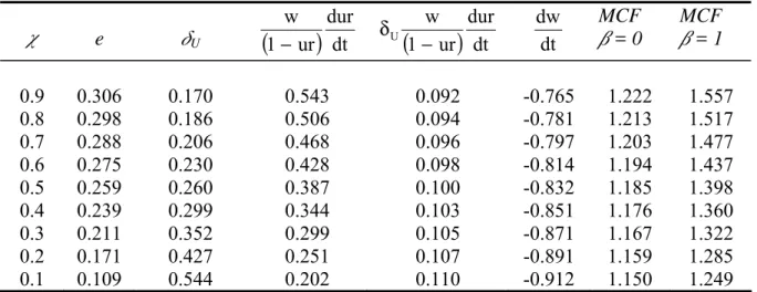
Table 1 shows that if the detection rate was 0.90, the corresponding cost of effort
would have to be 57.9 percent of the wage rate to generate the observed labour market
equilibrium. With these values, about three-quarters of the wage tax would be borne by
employees through a lower wage rate. The MCF would be 1.56 if profit income has the
same distributional weight as labour income. Since the MCF in a competitive labour
market with full employment and a fixed labour supply is 1.00, we can see that the
distortion caused by unemployment adds 0.56 to the MCF if the detection rate is high.
However, the table shows that with lower values for (, and correspondingly lower values
“only” 0.25 to the MCF. So while the effect of incorporating unemployment in the
calculation of the MCF is quite sensitive to the chosen values of the ( and e, it increases
the measured MCF by a significant amount even when the ( is low. The reason for the
decline in the MCF as the ( and e values decline is that although the distortion from
unemployment, U, increases, more of the tax burden is shifted to workers and therefore
the tax increase has a smaller effect on the overall level of unemployment. In other
words, the unemployment distortion per dollar of tax revenue is relatively constant, at
around 0.10, when ( varies from 0.9 to 0.1 and the MCF declines because the loss of
labour income per dollar of additional tax revenue declines.
Table 1 also shows the calculated values of the MCF when the distributional
weight on profit is zero. These MCFs are, not surprisingly, lower because the costs of tax
increases that are borne by firms are “ignored” in these calculations. These values for the
MCF also declined as ( and e decline, but within a narrower range from 1.15 to 1.22.
The model indicates that it may be important to incorporate the distortion caused
by unemployment in the calculation of the MCF. While we have used the framework of
the Shapiro-Stiglitz model to calculate U, dur/dt, and dw/dt terms, the results from
econometric studies on the impact of payroll taxes on labour markets could be used
instead, and this might narrow the range of values for the estimated MCF.
3.0 The Optimal Flat Tax
Einstein is reputed to have said “Nothing is as complicated as income tax.” From
this remark, we may speculate that Einstein tried to solve the optimal income tax
to the optimal income tax developed by Mirrlees (1971) is very complicated because
Mirrlees imposed very few restrictions on the structure of the income tax. Few
predictions come out of the general optimal income tax model, other than that the
marginal tax rate should be zero for the taxpayer with the highest wage rate and positive
for other taxpayers. Slemrod et al. (1994) tackled a more restrictive version of the
optimal income tax problem. They restricted the government’s choices to the tax rates in
two tax brackets and a lump-sum demogrant. Using a numerical simulation model, the
authors found, for a wide variety of parameter values, that the optimal two bracket
income tax has a lower marginal tax rate in the higher tax bracket. However, this result
might be specific to the type of utility function that they used to model individuals’
labour leisure decisions. Furthermore, they did not derive any analytical expressions
describing the properties of the optimal two bracket income tax. Hence the relationship
between the optimal income tax and the concept of the SMCF is not well articulated in
the literature, except in the work of Saez (2001).
In this section, we will impose even more structure on the optimal income tax
problem than Slemrod et al. (1994) by focusing on the optimal “flat tax”, i.e. an income
tax in which the marginal income tax rate in the first tax bracket is zero and the marginal
income tax rate in the second bracket is positive. The government’s only policy variables
are X1, which determines the size of the first bracket, and m2, the marginal tax rate on
income in excess of X1. We take the government’s expenditures (including income
transfer programs) as given. In other words, we do not include a lump-sum transfer to all
individuals as policy variable of the government. Imposing this structure on the optimal
expressions for the social marginal cost of funds (SMCF) for the two policy instruments,
X1, and m2. Hopefully, this will give some insights into the nature of the solution to the
more general income tax design problem. Second, the optimal design of a flat tax is an
interesting policy question in its own right because some economists, such as Hall and
Rabuska (1995) have advocated the adoption of a flat tax for the United States. Indeed,
Alberta’s provincial income tax is a flat tax, with an exemption level of $14,337 and a
marginal tax rate of 10 percent in 2004.
We derive the optimal flat tax by developing expressions for the SMCF using the
framework described in Dahlby (1998), except that it now assumed that there is a
continuous distribution of wage rates among the taxpayers. Suppose that the wage rate
varies between 0 and wtop. Let F(w) be the cumulative distribution function for wage
rates, with F(0) = 0 and F(wtop) = 1. The density function will be denoted by f(w). The
total population of individuals will be normalized to equal one.
Individuals have an identical utility function U(C, L), where C is consumption
and L is total labour supplied with UC > 0 and UL < 0. Let Y = wL be the individual’s
income. (Non-labour market income is assumed to be zero.) The individual’s
consumption opportunities are given by:
(
1)
12
1
X Y for X Y m Y C
X Y for Y
C
> −
− =
≤ =
(19)
The individual’s preferences over consumption and income are given by U(C, Y/w), and
the slope of an individual’s indifference curves in (C,Y) space is –(UL/UC)(1/w). This
implies that individuals with higher wage rates have less steeply sloped indifference
curves. Intuitively, for any (C,Y) combination, a high wage person needs to work fewer
consumption to compensate for the additional effort required to earn that additional dollar
of income. We can also represent individuals’ preferences using the indirect utility
function V((1 - m)w, Z) where m is zero if Y < X1 and m = m2 if Y > X1. The
individual’s virtual income is Z = mX1, with Z = 0 if Y [ X1 and Z= m2X1 if Y > X1.
With a continuous distribution of wage rates across individuals, some taxpayers
will find it optimal to earn X1 where there is a kink in their income–consumption
opportunity locus. This possibility is illustrated in Figure 2 where individuals with wage
rates ranging from w1 to w2 have indifference curves that are tangent at kink in their
consumption-income opportunity curve at X1. These wage rates are defined by the
following equations: ⎟⎟ ⎠ ⎞ ⎜⎜ ⎝ ⎛ ⎟⎟ ⎠ ⎞ ⎜⎜ ⎝ ⎛ − = 1 1 1 C 1 1 1 L 1 w X , X U w X , X U
w (20)
(
2)
2 1 1 C 2 1 1 L 2 m 1 1 w X , X U w X , X U w − ⎟⎟ ⎠ ⎞ ⎜⎜ ⎝ ⎛ ⎟⎟ ⎠ ⎞ ⎜⎜ ⎝ ⎛ − = (21)
The total number of individuals who earn exactly X1 is F(w2) – F(w1), and the total
number of taxpaying individuals is 1 – F(w2). An increase in X1 (holding m2 constant)
will increase w1 and w2 because individuals with higher wage rates have less steeply
sloped indifferences curves, and similarly, an increase in m2 will increase w2.
The government’s total tax revenue is equal to:
[
]
(
)
∫
− − = top 1 2 2 w ) X , m ( w 1 22 wL(1 m )w,Z X f(w)dw
m
where L[(1 – m2)w, Z] is the labour supply function of a taxpayer who receives a wage
rate of w. The government can increase revenue by raising m2 or by decreasing X1. We
begin by developing a measure of the marginal social cost of raising revenue by
decreasing X1. We then develop an expression for the SMCF of increasing m2
Applying Leibnitz’s rule, the derivative of (22) with respect to X1 is:
( )
(
[
]
)
∫
−∫
− − − = top 2 top 2 w w ww 2 2 2 2 1 2
1 2 2 1 2 1 ) w ( f X Z , w ) m 1 ( L w m dX dw dw ) w ( f m dw w f dX dZ dZ dL w m dX dR (23)
For taxpayers, i.e. individuals with w > w2, an increase in X1 is equivalent to a lump-sum
tax cut of m2dX1, and the first term reflects the income effect of this tax cut on the
individuals’ supply of labour. The second term is the decline in revenues from an
increase in X1, given the number of individuals in tax bracket two. The last term is the
effect of an increase in X1 on w2, but this effect is zero because an individual with a wage
rate of w2 earns X1. We will denote the income effect for an individual earning a wage
rate w by (w) = (1 – m2)wdL/dZ, and the effect of an increase in X1 on revenues can be
written as:
[
]
∫
θ− + − − = top 2 w w 2 2 2 2 2 1 dw ) w ( f ) w ( m 1 m m ) w ( F 1 m dX dR (24)
The average income effect for taxpayers will be defined as:
∫
θ − = θ top 2 w w 22 (w)f(w)dw
) w ( F 1 1 ) w ( (25)
Consequently, the effect on tax revenues of an increase in X1 can be expressed in terms
of the average income effect among individuals earning more than w2 as:
[
]
⎟⎟ ⎠ ⎞ ⎜⎜ ⎝ ⎛ θ − − − −= (w )
We will use the general social welfare function S(V(w, Z)) to reflect a
government’s distributional preferences. It will be assumed that the distributional
weights that are implicit in the social welfare function, (w) = SVVZ(w, Z), reflect
pro-poor preferences. Otherwise, the government would want to set X1 [ 0. It will be
convenient to decompose social welfare as:
∫
∫
∫
⎟⎟ + − ⎠ ⎞ ⎜⎜ ⎝ ⎛ ⎟ ⎠ ⎞ ⎜ ⎝ ⎛ + = top 2 2 1 1 w w 2 w w 1 1 w0 w f(w)dw S(V((1 m )w,Z))f(w)dw
X , X U S dw ) w ( f )) w ( V ( S S (27)
where the first term reflects the well-being of individuals who do not pay the tax, the
second term reflects the well-being of individuals who are the kink in the
income-consumption curve, and the third term reflects the well-being of taxpayers. Applying
Leibnitz’s rule, the effect of an increase in X1 can be written as:
(
)
(
)
∫
∫
+ − ⎟ ⎠ ⎞ ⎜ ⎝ ⎛ + ⎥ ⎦ ⎤ ⎢ ⎣ ⎡ − − ⎟⎟ ⎠ ⎞ ⎜⎜ ⎝ ⎛ + ⎥ ⎦ ⎤ ⎢ ⎣ ⎡ ⎟⎟ ⎠ ⎞ ⎜⎜ ⎝ ⎛ − = top 2 2 1 w w 1 2 v w w 1 1 1 V 2 1 2 2 2 1 1 1 V 1 2 1 1 1 1 1 V 1 1 1 ) w ( f dX Z , w ) m 1 ( dV S dw ) w ( f dX w X , X dU S ) w ( f X m , w ) m 1 ( V w X , X U S dX dw ) w ( f w X , X U ) w ( V S dX dw dX dS (28)The first two terms in this expression are equal to zero and therefore the effect of an
increase in X1 on social welfare is measured by the third term―the effect of an increase
in X1 on the well-being of individuals at the kink―and fourth term―the effect on the tax
paying individuals. For the taxpaying individuals, the marginal benefit from an increase
in X1 is simply m2. For the individuals who are at the kink, the marginal benefit from an
) w ( mb U w U U 1 U dX dU X C C L C 1 = ⎥ ⎥ ⎥ ⎥ ⎥ ⎦ ⎤ ⎢ ⎢ ⎢ ⎢ ⎢ ⎣ ⎡ ⎟⎟ ⎠ ⎞ ⎜⎜ ⎝ ⎛− − = (29)
Note that the mbX will vary from zero, for individuals earning w1, to m2 for individuals
earning w2. The mbX for individuals who earn between w1 and w2 is less than m2 because
these individuals are “off their labour supply curves” and consuming too much leisure.
We will define the smbX(w1, w2) as the distributionally-weight average mbX for
individuals at the kink where:
dw ) x ( f ) w ( mb ) w ( ) w ( F ) w ( F 1 ) w , w (
smb w X
w 1 2 2 1 X 2 1
∫
β −= (30)
Therefore the effect of an increase in X1 on social welfare can be written as:
[
F(w ) F(w )]
(w )m[
1 F(w )]
smb dX dS 2 2 2 1 2 X 11 − + β −
= (31)
where β(w2)is the average distributional weight among individuals earning more than
w2:
∫
β − = β top 2 w w 22 (w)f(w)dw
) w ( F 1 1 ) w ( (32)
Combining (26) with (31), we obtain the following expression for the social marginal
cost of raising revenue through a reduction in X1:
[
]
[
]
[
]
⎟⎟ ⎠ ⎞ ⎜⎜ ⎝ ⎛ θ − − − − β + − = − = ) w ( m 1 m 1 ) w ( F 1 m ) w ( F 1 m ) w ( ) w ( F ) w ( F smb dX dR dX dS SMCF 2 2 2 2 2 2 2 2 1 2 X 1 1 X 11 (33)
Note that the first term in the numerator of this expression is the
income-consumption curve. The smb may be greater than X1 β(w2)m2if the distributional
preferences implicit in the social welfare function are sufficiently pro-poor. Therefore,
even though the number of individuals who are at the kink will likely be much smaller
than the number of taxpayers, this first term may be important in the measuring the
1 X
SMCF if preferences are sufficiently pro-poor. Note that in the absence of this term,
the expression for the
1 X
SMCF would be very similar to the expression for the MCF for a
lump-sum tax increase in the presence of a proportional wage tax. Equation (33)
indicates, not surprisingly, that the social marginal cost of raising revenue through
lowering X1 and imposing taxes on a larger percentage of the population will be lower
the stronger the average income effect.
The derivation of the SMCF proceeds in a similar fashion. First, taking the m2
derivative of tax revenue with respect to m2, we can obtain:
(
)
∫
∫
⎥ ⎦ ⎤ ⎢ ⎣ ⎡ + − − + − = top 2 top 2 w w w w 1 2 2 1 2 dw ) w ( f X dZ dL ) w ( ) w ) m 1 (( d dL w m dw ) w ( f X wL dm dR[
]
[
]
⎟⎟ ⎠ ⎞ ⎜⎜ ⎝ ⎛ θ ζ − η − − ζ − −= ˆ(w ) (w )
m 1 m 1 ) w ( F 1 ) w (
Y 2 2
2 2 2
2 (34)
where Y(w2) is the average income of the taxpayers:
∫
− = top 2 w w 22 wL(w,Z)f(w)dw
) w ( F 1 1 ) w (
Y (35)
ζ is the ratio of X1 to Y(w2), and ηˆ(w2)is the (uncompensated) income-weighted
average labour supply elasticity for taxpayers:
∫
η − = η top 2 w w 2 22 (w)f(w)dw
Taking the derivative of the social welfare function, we obtain:
[
]
[
]
(
)
∫
λ − = − β −β ζ=
− top
2 w
w v 1 2 2 2 2
2 ) w ( ) w ( ˆ ) w ( F 1 ) w ( Y dw ) w ( f X ) Z , w ( wL ) w ( S dm dS (37)
where )βˆ(w2 is the income-weighted average distributional weight for the taxpayers:
∫
β − = β top 2 w w 2 22 (w)f(w)dw
) w ( Y wL ) w ( F 1 1 ) w ( ˆ (38)
Combining (34) with (37), we obtain the following expression for the
2 m
SMCF :
[
ˆ(w ) (w )]
m 1 m 1 ) w ( ) w ( ˆ SMCF 2 2 2 2 2 2 m2 θ ζ − η − − ζ − ζ β − β = (39)
The roles played by each component of the SMCF can be easily identified. In the
numerator, the two s reflect the social cost of the tax rate increase. The first is an
income-weighted average value because individuals with higher incomes will have higher
tax increases. The second enters the formula with a negative sign because it reflects the
off-setting increase in virtual income that occurs when m2 increases. Since the increase
in virtual income is the same for each taxpayer, this is an unweighted average. It is
multiplied by because the increase in virtual income is larger when X1 is higher. In the
denominator, the (1 - ) component reflects the proportion of income, on average, that is
subject to the tax rate increase. The term in square brackets indicates the labour supply
responses, where ηˆ(w2)reflects the income-weighted average response to the decline in
taxpayers’ net wage rates. It is an income-weighted average because the labour supply
changes by high income taxpayers have a proportionately larger effect on tax revenues.
The ζθ(w2)term in square brackets reflects the reduction in labour supplies because of
relatively high and when the average income effect among taxpayers is relatively strong.
The optimal flat tax can be defined as the (m2, X1) combination that, for a given
level of tax revenue, maximizes the social welfare function. The optimal (m2, X1)
combination will be found by equating the
2 m
SMCF in (39) with the
1 X
SMCF in (33).
Note that this solution involves various parameters, such as ηˆ(w2), θ(w2), )βˆ(w2 , and
) w ( 2
β which are functions of w2 and therefore functions of m2 and X1. Therefore, it is
not possible to derive simple reduced-form equations for m2 and X1 for the most general
case where the labour supply responses and distributional weights vary with the
individuals’ wage rates. However, some insights can be gleaned by equating (33) with
(39), and solving for the m2/(1 – m2) ratio:
(
)
[
]
(
)
(
)
[
−]
β(
η−ζθ)
+(
−)
(
βη−βθ)
− β − β + β −
ζ − =
− F(w ) F(w ) ˆ 1 F(w ) ˆ ˆ
) w ( F 1 ˆ )
w ( F ) w ( F 1 m
1 m
2 kink
1 2
2 kink
1 2
2
2 (40)
where kink = smbx/m2, can be interpreted as the average effective distributional weight
that is applied to the individuals who are at the kink in the income-consumption curve.
The numerator in (40) can be interpreted as the marginal social gain from a lump-sum
transfer financed by a marginal tax rate increase, MTT . To provide an intuitive
interpretation of the denominator, we make the simplifying assumption that and are
constant, and using the Slutsky decomposition = c + to eliminate , we can obtain
the following:
θ β + η β
β =
− MTT
c LST
MTT
2 2
m 1
m
(41)
LST is the marginal social gain from a pure lump-sum transfer, or:
[
−]
β +(
−)
β=
Since the left-hand side of (41) is increasing in m2, we can interpret this relation as
indicating that the optimal marginal tax rate will be higher when (a) the marginal social
gain from a marginal tax rate financed transfer is higher relative to a pure lump-sum
transfer, (b) the income effect on earnings of a lump-sum transfer is large (in absolute
value) and (c) if the substitution effect of a wage rate increase is low. All of these factors
accord well with our intuition, but unfortunately (41) does not allow us to solve for m2
because MTT and LST both depend on m2 and X1.
3.1 Computing the Optimal Flat Tax
To gain more insight into the nature of the optimal flat tax, we have used the
model developed above to compute the optimal m2 and X1. Suppose individuals have the
following CES utility function:
U
(
1−α)
Cσ−1 σ
⋅ α(T−L)
σ−1 σ
⋅ +
⎡ ⎢ ⎣
⎤ ⎥ ⎦
σ σ−1
(43)
where T – L is the total amount of time available for leisure, " is the elasticity of
substitution between consumption of goods, C, and leisure, and α is a positive parameter
determining strength of the preference for leisure. Following Stern (1976), the
individual’s labour supply function will be equal to:
L
T Z α
1−α
(
)
⋅[(1−m) w⋅ ]⎡ ⎢ ⎣
⎤ ⎥ ⎦
σ
⋅ −
1 (1−m) w⋅ α
1−α
(
)
⋅[(1−m) w⋅ ]⎡ ⎢ ⎣
⎤ ⎥ ⎦
σ
⋅ +
(44)
θ
1−m ( ) w⋅
[ ]
− α
1−α
(
)
⋅[(1−m) w⋅ ]⎡ ⎢ ⎣ ⎤ ⎥ ⎦ σ ⋅
1 (1−m) w⋅ α
1−α
(
)
⋅[(1−m) w⋅ ]⎡ ⎢ ⎣ ⎤ ⎥ ⎦ σ ⋅ + (45)
It also implies that the individuals at the kink in the income-consumption locus will have
wage rates between:
σ ⎟ ⎟ ⎟ ⎟ ⎠ ⎞ ⎜ ⎜ ⎜ ⎜ ⎝ ⎛ − ⎟⎟ ⎠ ⎞ ⎜⎜ ⎝ ⎛ α − α = 1 1 1 1 1 w X T X 1 w (46) ⎟⎟ ⎠ ⎞ ⎜⎜ ⎝ ⎛ − ⎟ ⎟ ⎟ ⎟ ⎠ ⎞ ⎜ ⎜ ⎜ ⎜ ⎝ ⎛ − − ⎟⎟ ⎠ ⎞ ⎜⎜ ⎝ ⎛ α − α = σ 2 1 2 2 1 1 2 m 1 1 w ) m 1 ( X T X 1 w (47)
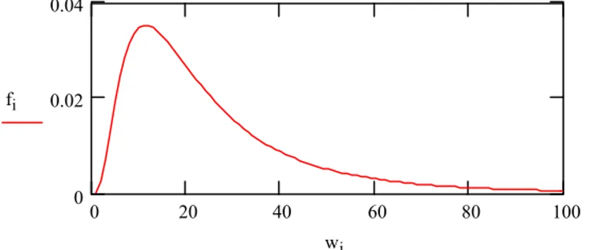
It was assumed that hourly wage rates follow a log normal distribution, where the mean
wage rate is w = 20. Therefore µw = ln(w) = 2.99573. The standard deviation of the
ln w was assumed to be σw = 0.75. The highest hourly wage rate was assumed to be
400. The corresponding distribution of wage rates across the population is shown in
Figure 3.
The preference parameters were selected in the following manner. It was
assumed that an individual earning the average hourly wage rate would choose to earn
$36,000 per year in the absence of taxation and that the income effect at the average
wage rate would be equal to -0.15. It was also assumed that α = 0.5. This implies that
T = 2117.65 and " = 1.579. This elasticity of substitution is considerably higher than the
would lead to relatively low values for the optimal marginal tax rate in our calculations.
As we will see, this is not the case. The social welfare function used to calculate the
distributional weights was S=
∫
(
1−ξ) (
−1 V(w))
1−ξf(w)dw, where > 0 reflects the strength of social preference for equality. The distributional weights were normalized sothat β(w)=1. The optimal flat tax was calculated such that it would yield the same
revenue as a 20 percent proportional tax on earnings.
Table 2 shows our results for = 0.5 and = 1.5. With = 0.5, the optimal
marginal tax rate is close to 41 percent, with an exemption level of $25,661 such that
only 57 percent of the population would pay the tax. However, 8.8 percent of the
population would at the kink in the income consumption curve. The average income of a
taxpayer would be $67,089. The uncompensated labour supply elasticities would be
positive but decline as the wage rate rose. The income-weighted average labour supply
elasticity would be 0.14169, which is within the usually range of values used in
simulating the labour supply effects of tax policies. Similarly the income effect of a
lump-sum transfer on earnings would decline (in absolute value) at higher income levels
with the average value for the income effect equal to -0.15425. The distributional
weights that underlie these computations ranged from 1.0628 at the bottom of the tax
bracket to 0.15953 at the highest income level. The model implies that even with
‘relatively moderate’ distributional preferences and with labour supply elasticities that are
in the normal range of values used in applied tax policies studies, the marginal tax rate
under the optimal flat tax would be significantly higher than the flat tax rates proposed
for the U.S. economy. In other words, the optimal flat tax may be considerably more
that with = 1.5 and distributional weights that range from 0.929 at the bottom of the tax
bracket to 0.1057 at the top of the tax bracket, the optimal flat tax rate would be over 50
percent.
Of course these computations are based on a simple model that used a rather
arbitrary distribution function for wage rates and ignored other features of taxpayer
behaviour, such as the ability of taxpayers, especially at high income levels, to receive
income in non-taxable, or low tax, forms such as fringe benefits. It has also ignored the
potential for under-reporting of earnings or tax evasion by working in the underground
economy. All of these factors are relevant in designing the optimal income tax and