www.geosci-model-dev.net/7/249/2014/ doi:10.5194/gmd-7-249-2014
© Author(s) 2014. CC Attribution 3.0 License.
Geoscientiic
Model Development
Methodological aspects of a pattern-scaling approach to produce
global fields of monthly means of daily maximum and
minimum temperature
S. Kremser, G. E. Bodeker, and J. Lewis
Bodeker Scientific, Alexandra, New Zealand
Correspondence to:S. Kremser ([email protected])
Received: 6 August 2013 – Published in Geosci. Model Dev. Discuss.: 13 September 2013 Revised: 4 December 2013 – Accepted: 23 December 2013 – Published: 30 January 2014
Abstract. A Climate Pattern-Scaling Model (CPSM) that
simulates global patterns of climate change, for a prescribed emissions scenario, is described. A CPSM works by quan-titatively establishing the statistical relationship between a climate variable at a specific location (e.g. daily maximum surface temperature, Tmax) and one or more predictor time
series (e.g. global mean surface temperature,Tglobal) –
re-ferred to as the “training” of the CPSM. This training uses a regression model to derive fit coefficients that describe the statistical relationship between the predictor time series and the target climate variable time series. Once that relationship has been determined, and given the predictor time series for any greenhouse gas (GHG) emissions scenario, the change in the climate variable of interest can be reconstructed – re-ferred to as the “application” of the CPSM. The advantage of using a CPSM rather than a typical atmosphere–ocean global climate model (AOGCM) is that the predictor time series re-quired by the CPSM can usually be generated quickly us-ing a simple climate model (SCM) for any prescribed GHG emissions scenario and then applied to generate global fields of the climate variable of interest. The training can be per-formed either on historical measurements or on output from an AOGCM. Using model output from 21st century simu-lations has the advantage that the climate change signal is more pronounced than in historical data and therefore a more robust statistical relationship is obtained. The disadvantage of using AOGCM output is that the CPSM training might be compromised by any AOGCM inadequacies. For the pur-poses of exploring the various methodological aspects of the CPSM approach, AOGCM output was used in this study to train the CPSM. These investigations of the CPSM method-ology focus on monthly mean fields of daily temperature
extremes (TmaxandTmin). The methodological aspects of the
CPSM explored in this study include (1) investigation of the advantage gained in having five predictor time series over having only one predictor time series, (2) investigation of the time dependence of the fit coefficients and (3) investigation of the dependence of the fit coefficients on GHG emissions scenario. Key conclusions are (1) overall, the CPSM trained on simulations based on the Representative Concentration Pathway (RCP) 8.5 emissions scenario is able to reproduce AOGCM simulations ofTmax and Tmin based on predictor
time series from an RCP 4.5 emissions scenario; (2) access to hemisphere average land and ocean temperatures as predic-tors improves the variance that can be explained, particularly over the oceans; (3) regression model fit coefficients derived from individual simulations based on the RCP 2.6, 4.5 and 8.5 emissions scenarios agree well over most regions of the globe (the Arctic is the exception); (4) training the CPSM on concatenated time series from an ensemble of simulations does not result in fit coefficients that explain significantly more of the variance than an approach that weights results based on single simulation fits; and (5) the inclusion of a lin-ear time dependence in the regression model fit coefficients improves the variance explained, primarily over the oceans.
1 Introduction
computationally demanding and expensive to run, typically only a limited number of long-term simulations, for only a few GHG emissions scenarios, can be conducted in support of any scientific study. However, a fully probabilistic assess-ment of future regional climate change and its potential im-pacts requires simulations of climate change that span a wide range of possible future GHG and aerosol emissions. Simple climate models (SCMs), while computationally less expen-sive than AOGCMs, provide only annually and globally (or sometimes hemispherically) averaged time series of surface temperature and therefore cannot represent spatial patterns of changes in surface climate variables (Mitchell, 2003). SCMs can, however, simulate changes in global annual mean surface temperature (Tglobal) for any prescribed GHG and
aerosol emissions scenarios and can be tuned to emulate any specific AOGCM (Frieler et al., 2012; Meinshausen et al., 2009).
To generate fields of climate variables for a range of emis-sions scenarios, the climate pattern-scaling method was de-veloped (Mitchell et al., 1999; Mitchell, 2003) and encoded, in what is referred to, in this study, as a climate pattern-scaling model (CPSM). This CPSM provides a tool to con-duct regional-scale climate projections for a range of climate variables such as daily maximum and minimum temperatures (TmaxandTmin) for a wide range of GHG emissions
scenar-ios. Using maximum and minimum temperatures as opposed to monthly mean temperature is more useful for some spe-cific applications, for example, for agriculture and for public health officials tasked with providing warnings of extreme climate events. Crop growth, and therefore crop yields, are more sensitive to maximum and minimum temperature than to daily mean values. Furthermore, probabilistic projections of Tmax andTmin provide means to estimate future energy
demand (e.g. increase/decrease in the usage of air condition-ing or heatcondition-ing). As a result, this study uses monthly means of daily maximum and minimum temperature rather than monthly means of daily mean temperature to explore the methodological aspects of climate pattern scaling. The cli-mate pattern-scaling method has been used to capture the statistical relationship between time series of surface climate variables (such as maximum and minimum temperatureTmax
andTmin) and predictor time series (typicallyTglobal), based
either on measurement time series or on AOGCM output – referred to as the “training” of the CPSM. Those statistical relationships can then be used to project the spatial pattern of changes in a climate variable for different emissions sce-narios, or for future time periods, that were not covered by the data set used for the training – referred to as the “appli-cation” of the CPSM. Once the data required for the train-ing are available, the pattern-scaltrain-ing approach is computa-tionally inexpensive and therefore provides a mechanism for representing a more complete range of uncertainties associ-ated with climate projections that arise from equally probable emissions scenarios and from uncertainties in our knowledge of key parameters in the climate system. The pattern-scaling
method is based on the assumption that the local response of a given climate variable, such as daily maximum and min-imum surface temperatures (TmaxandTmin), and to a lesser
extent precipitation, can be statistically related to the change in a more easily modelled climate variable such as Tglobal
(Giorgi et al., 2005; Frieler et al., 2012), irrespective of the forcing that caused the change inTglobal. Non-linearities can
arise, for example, as a result of local climate change depend-ing on the rate of global mean temperature change in addition to the magnitude of the change (Mitchell, 2003). Giorgi et al. (2005) showed that the non-linear fraction of the climate change signal tends to decrease with increasing magnitude of the signal, suggesting that the linear response assumption will be increasingly robust as the climate change signal be-comes more pronounced.
Different methods have previously been developed to de-termine the statistical relationship between the climate vari-able of interest and its predictors (e.g. Huntingford et al., 2000; Mitchell, 2003; Ruosteenoja et al., 2007). Linear least squares regression models, in general, produce more robust statistical results than an approach that uses two time-slice simulations separated in time (Mitchell, 2003; Ruosteenoja et al., 2007).
In this study, a CPSM is used to explore some of the methodological aspects of the pattern-scaling approach that have not been, to our knowledge, investigated in detail in the existing literature. The motivation is to define more clearly where the assumptions underlying the CPSM approach are valid, possible reasons for breakdowns in those assumptions, and potential strategies to improve the CPSM approach to mitigate the effects of methodological weaknesses. Follow-ing the best practice approaches outlined in Mitchell et al. (1999), Huntingford et al. (2000), and Mitchell (2003), the climate pattern response is obtained by using a linear least squares regression model to relate the anomaly in a surface climate variable (the predictand) to the anomaly in the dictor. By using anomalies in both the predictor and the pre-dictand with respect to the same baseline period, more sta-tistically robust results are obtained than in the case where absolute values are modelled. CPSM generated patterns of change can be added to an observations-based climatology over the baseline period to obtain absolute values of the cli-mate variable of interest. Throughout this paper, unless oth-erwise specified, all anomalies are with respect to the 1961– 1990 mean as this is the baseline period recommended by the World Meteorological Organization (WMO) Commission on Climatology and is used as the climatological baseline in cli-mate impact studies (Parry et al., 2007).
In this studyTglobal′ , where the prime denotes that it is an anomaly, is usually used as the predictor. In addition to using
Tglobal′ as a predictor, and unlike previous studies, the CPSM
of the CPSM explored in this study (see Sect. 4) is the ad-vantage gained in having five predictor time series (T′
global,
the hemispheric ocean and land temperatures) over having only one predictor time series (Tglobal′ ).
The surface climate variables used to explore selected fea-tures of the CPSM are the monthly means of daily maxi-mum and minimaxi-mum temperature (TmaxandTmin). While the
regression model applied in the CPSM training could use ob-servational data as input, the climate signal to date has been weaker than the signal expected over the 21st century. There-fore, the CPSM has been trained on output from the Met Of-fice Hadley Centre Earth System Model (HadGEM2-ES) per-formed under the Coupled Model Intercomparison Project phase 5 (CMIP5) in support of the Intergovernmental Panel on Climate Change (IPCC) 5th assessment report (see Ap-pendix A). The results presented in this paper are therefore contingent on only a single AOGCM being used and only for simulations to 2100.
The training of the CPSM is described in detail in Sect. 2 which includes the construction of the regression model, how autocorrelation in the regression model residuals is ac-counted for to obtain a robust estimate of the regression model fit coefficient uncertainties, a demonstration of the CPSM training, how seasonality in the fit coefficients is cap-tured, and examples of global maps of fit coefficients. The application of the CPSM is described in Sect. 3. The first of the methodological issues explored in this paper – the value obtained by including additional predictors (basis functions) in the regression model – is documented in Sect. 4. This sec-tion includes a discussion of the need to orthogonalise the multiple basis functions, presents an example of the use of a multiple basis function CPSM, and an assessment of the value of including additional basis functions. The underlying assumption in the CPSM approach of linearity across scenar-ios in the response of the predictor to the predictand(s) is ex-plored in Sect. 5. The training of the CPSM can be performed on more than one simulation, either concatenated (the super-ensemble approach) or in parallel with appropriate weighting of the different outcomes. The methodological aspects of the choices involved in the use of multiple simulations for CPSM training are detailed in Sect. 6. The possibility of time depen-dence in the fit coefficients is examined in Sect. 7. A discus-sion of the results and the concludiscus-sions drawn appear in the final section of the paper.
2 Training of the CPSM
2.1 Model construct
The most simple construct for the regression model underly-ing the CPSM is
Fi,j′ (y, m)=αi,j(m)×Tglobal′ (y)+Ri,j(y, m), (1)
whereF′is the anomaly field of the climate variable of
inter-est (eitherT′
maxorTmin′ in this study) in year (y) and month
(m) and where the subscriptsiandj refer to longitude and latitude indices,Tglobal′ is the annual global mean tempera-ture anomaly andRi,j(y, m)is the residual time series.
Un-certainties on the fit coefficients are derived from the diago-nal elements of the covariance matrix as described further in Bodeker et al. (1998).
2.2 Accounting for autocorrelation in the residuals
Ri,j(y, m)in Eq. (1) is the residual (i.e. that part of the signal
not explained byαi,j(m)×Tglobal′ (y)). Due to the timescales
associated with the climate system, temporal correlation be-tween these residuals is expected, that is, if thenth residual is positive there is a greater chance of the (n+1)th residual be-ing positive rather than negative. This autocorrelation (Tiao et al., 1990; Weatherhead et al., 1998; Reinsel et al., 2005) implies that the data to which the regression model is being fitted are not completely independent and as a result there are effectively fewer independent values than the number of months of data available. This effectively increases the un-certainty on the fit coefficients. If this autocorrelation is not correctly accounted for in the regression model, the uncer-tainty on the fit coefficients will be underestimated (Tiao et al., 1990). Here, a first order autocorrelation model is used, where thenth residual is correlated against the (n−1)th resid-ual to determine the coefficient of autocorrelation. The de-rived coefficient is then incorporated into a revised estimate of the uncertainty on the data to which the model is fitted, as described in Tiao et al. (1990). This autocorrelation also varies with season and this seasonality is captured in the re-gression model.
2.3 Demonstration of CPSM training
To demonstrate the use of this very simple regression model, time series of Tmin′ at Alexandra, New Zealand (45.2◦S, 169.4◦E), extracted from a HadGEM2-ES simulation under Representative Concentration Pathway (RCP) 4.5 emissions (see Appendix A), andTglobal′ from the same model and emis-sions scenario, are shown in Fig. 1.
Unforced variability within a model simulation (e.g. aris-ing from El Niño events) can cause theTmin′ andTglobal′ time series to be correlated in a way that is unique to this par-ticular simulation (e.g. a HadGEM2-ES simulation based on RCP 4.5 emissions). With different initial conditions, how-ever, this particular simulation might produce an equally validTglobal′ time series but with weaker correlation than the time series shown in Fig. 1. In the example presented in Fig. 1 the short-term correlation between the orange and cyan traces appears to be small but the correlation can be greatly exacer-bated if additional predictors are included in the CPSM (see Sect. 4). When it comes to the application of the CPSM, the
! !
Fig. 1. January mean daily minimum temperature anomalies
(with respect to 1961–1990) at 45.2◦S, 169.4◦E extracted from a
HadGEM2-ES simulation under RCP 4.5 emissions (orange), the time series smoothed using the Savitzky–Golay filter (red), the an-nual mean global mean surface temperature anomaly (with respect
to 1961–1990) time series (Tglobal′ ) from the same model
simula-tion and emission scenario (pale blue), and the smoothedTglobal′
time series (blue).
most likely output from a SCM that captures only long-term, forced climate change, and therefore it is essential that none of the correlation betweenTmin′ andTglobal′ arises from short-term, unforced variability. The focus of this study is to apply the CPSM to simulate the underlying forced climate change. To this end, theTmin′ andTglobal′ time series are fil-tered (smoothed) to reduce unforced variability;T′
min time
series are smoothed individually across each calendar month to avoid smoothing away the annual cycle. The time series smoothed with a Savitzky–Golay filter (Savitzky and Golay, 1964; Press et al., 1989), which was found to work well for this application, are also shown in Fig. 1.
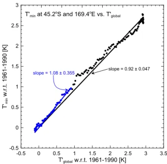
The regression of January meanTmin′ at Alexandra, New Zealand (45.2◦S, 169.4◦E), againstTglobal′ is shown in Fig. 2, where the smoothed AOGCM time series shown in Fig. 1 have been used.
Regression model fits (solid lines in Fig. 2) are shown for two time periods, namely, (1) 1961–2012 to indicate how a fit might look were it is based on observations alone, and (2) 1961–2100 to indicate the result obtained using a much longer time series. A fit using only 1961–2012 data has the benefit that it could be based on observations and therefore not subject to model inadequacies. However, gap-free monthly mean data would not be available for all loca-tions for this period. Access to a longer time series, span-ning a greater range inTmin′ andTglobal′ , produces fit coef-ficients with smaller uncertainties (see fit coefficient values in Fig. 2) but are, of course, subject to any inadequacies of the AOGCM that was used to generate the time series. It be-comes a judgment call on the part of the user whether to use
!
"
# $ % &
Fig. 2. Smoothed January mean daily minimum temperature
anomalies at 45.2◦S, 169.4◦E regressed against annual mean
global mean surface temperature anomalies. The data shown are from a single simulation, with the blue dots showing data from 1961 to 2012 and the black dots showing data from 2013 to 2100. All anomalies are with respect to the 1961–1990 baseline. Regression model fits (solid lines) are shown for 1961–2012 to indicate how a fit might look were it based on observations (blue solid line) alone and 1961–2100 to indicate the result obtained using a much longer time series (black solid line).
a (shorter) observational record or a (longer) model record to calculate the regression model coefficient(s) that constitute the training of the CPSM. Hereafter, output from HadGEM2-ES simulations are used to train the CPSM (more detailed in-formation on the HadGEM2-ES model and simulations used in this study is given in Appendix A).
2.4 Fitting for seasonality
TheTglobal′ time series are obtained at annual resolution, as
the regression model fit coefficient in a Fourier series, that is,
α(m)=α0+ M
X
k=1
[α2k−1sin(2π×k×m/12)
+α2kcos(2π×k×m/12)], (2)
wheremis the month of the year andM is the number of Fourier pairs in which the fit coefficients are expanded (Ran-del and Cobb, 1994; Bodeker et al., 1998; Reinsel et al., 2005). The value ofMcan be set depending on the seasonal structure expected in the fit coefficients. For the analysis pre-sented below,Mwas set to three for all Fourier expansions. In addition to reducing the number of fit coefficients by a factor of 7/12 compared to the approach of fitting the regres-sion model separately in each month, the method used here also reduces the statistical uncertainty on the derived fit co-efficients (we now refer to the fit coco-efficients as plural since the application of Eq. (2) results in more than one coefficient that relatesF′toTglobal′ ).
2.5 Global maps
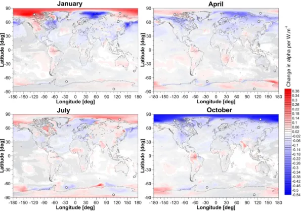
Global spatial patterns ofαfor bothTmax′ andTmin′ together with their 1σ uncertainties are shown in Fig. 3. The fit co-efficients were obtained from the fit of Tglobal′ to Tmax′ and Tmin′ time series, respectively, where all time series were ex-tracted from the HadGEM2-ES RCP 4.5 simulation. The de-rivedαcoefficients are displayed for four selected months of the year.
The α fit coefficient captures the “magnification” of re-gional temperature change compared to the global mean sur-face temperature change, that is, a value ofα=4 forTmax′ indicates that a 1◦C increase inTglobal′ corresponds to a 4◦C increase inTmax′ at that location. The largestα coefficients occur at high latitudes over the Northern Hemisphere in Jan-uary and October (i.e. it is over the Arctic in winter when feedback processes in the climate system are most efficient in amplifying the effects of increases in GHG emissions). This indicates that the CPSM faithfully emulates the Arctic amplification observed in HadGEM2-ES (i.e. that the mag-nitude of the temperature change in the Arctic in response to a change in global climate forcing tends to be significantly larger than the magnitude of the global mean temperature change) (Moritz et al., 2002). Arctic amplification is most pronounced in autumn and winter (Serreze and Barry, 2011) which is consistent with the results shown here (i.e. greaterα and therefore greater sensitivity inT′
maxandTmin′ toT
′
global).
Southern Hemisphere αcoefficients also maximize at high latitudes, particularly around the Antarctic Peninsula, but do not show values as high as over the Arctic. The larger val-ues of α in April over the Weddell Sea may be related to long-term changes in sea ice. The results presented in Fig. 3 indicate that the climate feedbacks that amplify the global signal in the Arctic (e.g. changes in the ice–albedo feedback) are stronger than those active in the Antarctic. Overall, as
expected due to the differences in the heat capacity of ocean and land, theαcoefficients are larger over land than over the ocean showing that land masses are expected to show greater changes inTmax′ and Tmin′ with changes in Tglobal′ than the oceans.
Note that some regions in Fig. 3 exhibit negativeα coeffi-cients, typically over the sub-polar oceans. Negativeαvalues indicate a temperature trend opposite in sign to that ofTglobal′ . This could occur, for example, if changes in the ocean heat transport in a particular model simulation cause some regions of the ocean to warm at the expense of other regions which cool.
2.6 Area averaging
In much the same way that regression model fit coefficients in neighbouring months are related (suggesting the use of Fourier expansions to capture the seasonal coherence), fit coefficients in neighbouring grid cells are also expected to be closely related. Throughout this paper Eq. (1) is applied in isolation in each grid cell of the AOGCM and therefore does not inherently capture the geospatial correlation of the fit coefficients. This may result in structure in the fit coeffi-cients that is a function of the specific emissions scenario(s) on which the CPSM is trained and therefore not represen-tative of the structure of the response of the climate system in general. Previous analyses (e.g. Frieler et al., 2012) have used area averaging of the fields prior to training the CPSM to avoid fine-scale structure in the fit coefficients. However, this results in sharp discontinuities between regions when the CPSM is used in application mode. An alternative ap-proach is to further expand the model fit coefficients (e.g. theαk in Eq. 2) in spherical harmonics where again the
or-der of the meridional and zonal expansions can be selected to capture the broad-scale features of the fit coefficient fields but to smooth over the fine-scale features. The spherical har-monic expansion recognises the geospatial correlation in the fit coefficients between neighbouring grid cells. This also re-quires only a single fit of the regression model to the data. In this study, such an approach has not been followed since it is our goal to explore the issues that may arise when applying the regression model in the traditional way (i.e. separately in each grid cell).
3 Application of the CPSM
Fig. 3. Global maps ofαfit coefficients forTmax′ (left column) andTmin′ (right column) for four selected months of the year. The coefficients
were obtained by fittingTglobal′ (Eq. 1) toTmax′ andTmin′ time series from the HadGEM2-ES RCP 4.5 simulation. The colour scale shows
the value ofαwhile the overlaid contours show the 1σuncertainties onα(hatch marks on the contours show the direction towards smaller
uncertainties). Regions in red show whereTmax′ andTmin′ are warming faster than the global mean surface temperature and regions in blue
where they are warming slower than the global mean surface temperature and possibly even cooling (negativeαvalues).
series from the AOGCM used to train the CPSM, andTglobal′ time series from the SCM for the same emissions scenarios, are identically correlated. Because the SCM and AOGCM may have different climate sensitivities, scaling of the SCM data may be required. This introduces some uncertainty. To avoid the additional complexity and uncertainty introduced by such scaling ofTglobal′ from a SCM, in this paper that ex-plores the methodological aspects of climate pattern-scaling,
Tglobal′ time series are extracted from simulations generated
by the same AOGCM as used in the training, but from differ-ent emissions scenarios, were used in application mode.
The use of the CPSM in application mode is demonstrated in Fig. 4.
!!
Fig. 4. Annual mean Tmin′ smoothed time series at Alexandra,
New Zealand (45.2◦S, 169.4◦E), from a HadGEM2-ES
simula-tion based on RCP 4.5 emissions (light green), together with its
regression model fit (dark green). Theαfit coefficients, resolved by
season, are shown in the lower right inset. When these fit
coeffi-cients are used together with theTglobal′ predictor time series from
HadGEM2-ES simulations under the RCP 2.6 and RCP 8.5 scenar-ios they produce the dark red and dark blue curves, respectively. The
actual annual mean RCP 2.6 and RCP 8.5 smoothedTmin′ time
se-ries at 45.2◦S, 169.4◦E are shown as light blue and light red lines,
respectively. The insert in the upper left shows the mean annual
cycle, calculated from the monthlyTmin′ time series, from 2090 to
2098 for all six time series.
levels required on the monthly meanTmin′ time series, used to derive weights within the regression model, were pro-vided as the standard deviations on the differences between the smoothed and unsmoothed time series for each calendar month. In this way, months exhibiting greater natural ability are given less weight than those with smaller vari-ability. The extent of the agreement between these CPSM derived time series and the original HadGEM2-ES time se-ries (underlying light blue and light red lines in Fig. 4) is in-dicative of the applicability of the CPSM. The CPSM tracks the original HadGEM2-ES output for the RCP 2.6 and RCP 8.5 simulations well, but tends to underestimate the magni-tude of the RCP 8.5 signal and overestimate the magnimagni-tude of the RCP 2.6 signal, suggesting possible non-linearities in the system. Previous studies have found that errors arising from pattern-scaling are much greater when scaling from low to high emissions scenarios than when scaling from high to low scenarios (Huntingford et al., 2000; Mitchell, 2003).
The seasonality of the fit coefficient (lower-right inset in Fig. 4) indicates thatTmin′ at this particular location, in late summer (January–March) increases almost as rapidly as the global mean temperature, but at only around half this rate in late winter. The upper-left inset in Fig. 4 demonstrates that this seasonality is consistent with what is seen in the smoothed raw HadGEM2-ES output.
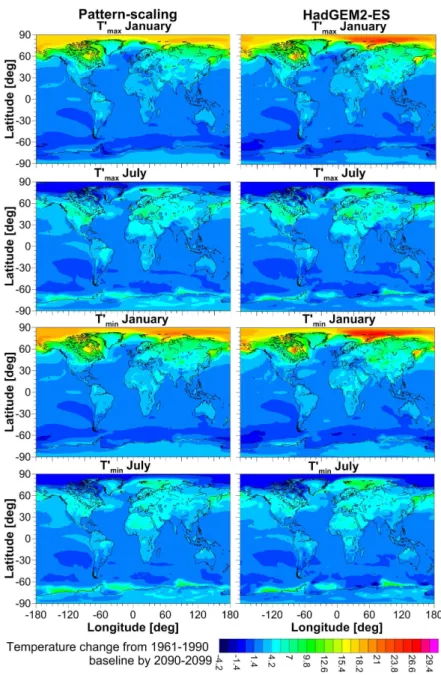
To further compare the results of the HadGEM2-ES RCP45 simulation with the generated fields by the CPSM, global maps of the decadal mean (2090 to 2099) of T′
max
andTmin′ for January and July are displayed in Fig. 5 (i.e. the change inTmax andTmin by the 2090s with respect to
the baseline period). Decadal means are shown to suppress the higher inter-annual variability across individual months displayed by HadGEM2-ES compared to output from the CPSM. The global pattern ofTmax′ andTmin′ derived from the CPSM output generally agrees well with the HadGEM2-ES simulation, although there are some regions (e.g. the Arctic Ocean) and periods (e.g. January) where the signal, that is, the change inTmax′ andTmin′ with respect to the baseline pe-riod 1961–1990, is more pronounced in HadGEM2-ES. This might be the result of simulation-specific decadal-scale un-forced variability in the HadGEM2-ES RCP 4.5 simulation which causes regional changes inT′
maxorTmin′ to be greater
than what is expected from theTglobal′ time series and theα fit coefficients obtained from the RCP 8.5 simulation. An-other reason for the unusual behaviour in this region may be that while two simulations may produce similarTglobal′ evo-lution, that evolution may result from different balances be-tween long-term and short-term climate forcing agents, for example, one simulation has high CO2emissions which are
significantly offset by high sulfate emissions while the sec-ond scenario has both lower CO2and sulfate emissions such
that theTglobal′ evolution in the two simulations is the same. A location outside of the region of sulfate aerosol-induced cool-ing would then be under the influence of different CO2 but
with the sameTglobal′ across the two simulations. The effects of such differences in short-lived radiative forcing agents has not been quantitatively assessed in this study but are recog-nised as a potential factor that may affect the linearity of the regression model fit coefficients across scenarios.
The overall close agreement between the CPSM and HadGEM2-ES fields provides evidence that the CPSM trained on RCP 8.5 simulations is able to provide a robust simulation ofTmax′ andTmin′ time series globally for the RCP 4.5 emissions scenario.
There are a number of methodological aspects of the CPSM approach which extend or improve upon the simple pedagogical example given above. These methodological as-pects are explored in greater detail in Sects. 4 to 7 below.
4 Additional basis functions
4.1 Regression model structure with multiple basis
functions
Some SCMs, such as MAGICC, in addition to generating time series of annual mean global mean surface temperature, are also able to generate annual mean hemispheric mean land
(TSH land andTNH land) and ocean (TSH ocean and TNH ocean)
Fig. 5. The change inTmax′ andTmin′ between 1961–1990 and 2090–2099 in January and July derived from the CPSM (left column) and extracted from the HadGEM2-ES model (right column). Both model simulations are based on RCP 4.5 emissions, while the CPSM was trained on HadGEM2-ES simulations based on RCP 8.5 emissions.
as Tx′. These time series, when used as additional predic-tors, may provide a degree of explanatory power above what would be available when onlyTglobal′ is used as the predic-tor. The construction of the regression model underlying the CPSM would then be of the form:
Fi,j′ (y, m)=αi,j(m)×Tglobal′ (y)+βi,j(m)×TNH land′ (y)
+γi,j(m)×TNH ocean′ (y) (3)
+δi,j(m)×TSH land′ (y)+ǫi,j(m)
×TSH ocean′ (y)+Ri,j(y, m).
As before, all predictor and predictand time series are smoothed with a Savitzky–Golay filter.
4.2 Orthogonalising multiple basis functions
Fig. 6. Plots of the orthogonalised Tx′⊥ time series from the RCP 4.5 simulation ofTmax′ together with their associated annual mean
regression model fit coefficients.⊥denotes that the basis functions have been orthogonalised. Double hatching shows where the coefficients
are not statistically significantly different from zero at the 1σ level and single hatching where they are not different from zero at the 2σlevel.
The thin black line on each map indicates the 0.0 value. Minimum values are shown in blue and pass through cyan, green, yellow and orange to maximum values in red (see lower left corner in each panel).
basis function can offset the negative signal from another to track a small change in the predictand. In addition to preclud-ing a physical interpretation of the fit coefficients, this lack of orthogonality can result in unstable behaviour of the CPSM if theTx′ time series are obtained from an SCM which may have a slightly different distribution of heat content between ocean and land than in the AOGCM on which the CPSM was trained (hereafter referred to asT′
x⊥). The non-orthogonality
of the basis functions also precludes a direct comparison of regression model fit coefficients obtained from training on AOGCM simulations from different emissions scenarios.
explained by the existing basis functions, and that coeffi-cients obtained from fits to different emissions scenarios are directly comparable.
4.3 Demonstration of the use of multiple basis functions
The five basis function time series, extracted from a HadGEM2-ES RCP 4.5 simulation, were smoothed and or-thogonalised and are shown together with their associated re-gression model fit coefficients in Fig. 6. The fit coefficients were derived globally at every grid point by applying the re-gression model toTmax′ , where theTmax′ time series were also extracted from the HadGEM2-ES RCP 4.5 simulation.
The apparent decadal variability seen in the four time se-ries displayed in Fig. 6 (excludingTglobal′ ⊥, where the sub-script⊥indicates that the basis function has been orthogo-nalised) should not be confused with unforced decadal-scale variability in the climate system but rather seen as subtle decadal-scale departures from the monotonically increasing
Tglobal′ time series which may well be forced changes.
Fig-ure 6a shows that for the primary predictor (Tglobal′ ⊥), the associated regression model fit coefficient (αin Eq. 3) is ev-erywhere statistically significantly different from zero, max-imizing in the Arctic and with lowest values over the oceans consistent with what was shown in Fig. 3. When the shape of aFi,j′ time series (see Eq. 1) is simply a linear scaling of
Tglobal′ ⊥, all higher order fit coefficients are zero (the zero line
in all Fig. 6 panels is indicated with a thin black line). Care must be taken when attributing cause and effect in Fig. 6. For example, in this simulation, additional predictive power appears to be gained from the TNH Ocean′ ⊥ time series over the Arctic Ocean but also, interestingly, over the Southern Ocean where a longitudinal dipole in response to the orthog-onalisedT′
NH Ocean⊥ is apparent. Does this suggest that the
Northern Hemisphere ocean is a driver of variability inT′
max
off the Antarctic coast? This is unlikely. Rather the variability inTmax′ off the Antarctic coast, over and above what would be expected from changes inTglobal′ ⊥, is correlated with changes in the orthogonalisedTNH Ocean′ ⊥time series. Had the basis functions been orthogonalised in a different order, it is likely that different conclusions would be drawn.
While additional basis functions may provide additional predictive power (see below), the need to orthogonalise these basis functions obfuscates a physical interpretation of what sources of variability they represent. The exact morphology of the fit coefficients shown in Fig. 6 is also likely to be sim-ulation dependent and dependent on the degree of smoothing applied to theTx′ time series. Analyses with access to an en-semble of simulations made under the same boundary condi-tions might provide more robust results.
4.4 Assessing the value of using multiple basis functions
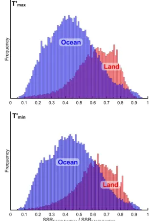
Two different versions of the CPSM were trained on Tmax′ and Tmin′ time series obtained from the HadGEM2-ES
Fig. 7. Histograms of the ratios of the SSR values for the five basis
functions CPSM (SSR5) to the one basis function CPSM (SSR1)
forTmax′ (upper panel) andTmin′ (lower panel). The SSR ratios
were determined for every grid point by dividing SSR5 by SSR1. The grid points and corresponding SSR ratios were assigned to be located over land or ocean and those values are shown in the his-tograms. SSR ratios shown here are based on all three RCP simu-lations, where the regression model has been trained separately on each RCP scenario.
simulations. In the first version onlyTglobal′ was used as a pre-dictor whereas in the second all fiveTx′⊥were used as pre-dictors. To derive a globally applicable measure of the dif-ferences between the two model constructs, the sum of the squares of the residuals (SSR) (i.e. the differences between the HadGEM2-ES time series and the time series produced from the regression model) were calculated for each model construct. For each AOGCM grid cell, the SSR value, calcu-lated from the CPSM with five basis functions (SSR5) was divided by the SSR value calculated from the model with a single basis function (SSR1). This was done for each of the three RCP scenarios for which simulations were available. The calculated SSR ratios for every grid point were assigned to be located either over land or ocean and the results forT′
max
andT′
min, for all RCP scenarios, are shown in the histograms
By using the hemispheric annual mean temperatures over land and ocean as predictors in addition to the global an-nual mean surface temperature, the SSR over land is typi-cally reduced by 25 % to 35 %, for bothTmax′ andTmin′ . Over the oceans, however, the SSR is typically reduced by about 50 % to 60 % when using additional information about hemi-spheric ocean and land temperatures as predictors. The re-sults suggest that while adding more basis functions to the regression model makes a physical interpretation of the as-signment of variability across the different basis functions difficult to interpret, it does result in a CPSM that is better able to track subtle changes inTmax′ and Tmin′ that are not simple linear scalings ofTglobal′ . Whether that additional skill is physically meaningful or just a statistical artefact requires further investigation. For the remainder of this paper the sin-gle basis function version of the CPSM (which is the more traditional version of the CPSM) is used to explore the re-maining methodological issues addressed in this paper.
5 Scenario dependence
The key assumption of the pattern-scaling approach is that the relationship between the predictors and the predictands is linear, that is, the regression model fit coefficients should, ideally, be robust properties of the climate system and should not depend on GHG emissions scenarios or vary with time. To test these assumptions, regression model fit coefficients were derived using all three RCP simulations available from the HadGEM2-ES model where onlyTglobal′ was used as the predictor time series. The seasonal cycles of theseαfit coef-ficients, together with their 1σuncertainties, for four selected sites forT′
maxand for four selected sites forT
′
min(one site in
common), are shown in Fig. 8.
The two Arctic sites showαpeaking in October or Novem-ber during the onset of sea-ice formation suggesting that long-term changes in sea ice in this season may be driving the large sensitivity ofTmax′ andTmin′ toTglobal′ . Interior sites in Greenland and Siberia showαpeaking around the begin-ning and end of winter suggesting that long-term changes in snow cover and hence surface albedo at these times may be driving the high values inα. At the beginning and end of the winter, the magnitudes ofαat both sites over the Arctic Ocean are greater than the magnitudes over the two interior sites. This amplified seasonal change in α over the Arctic Ocean indicates that the long-term changes in sea-ice extent and concentration have a stronger impact on the sensitivity ofT′
maxandT
′
mintoT
′
globalthan surface albedo changes over
land at high latitudes. The Southern Hemisphere mid-latitude site selected (Alexandra) showsαpeaking in summer (De-cember to February; see also Fig. 4) for bothTmax′ andTmin′ with the seasonal cycle inαbeing slightly more pronounced for Tmax′ . At the high southern latitude site over Antarctic sea ice (Weddell Sea),αpeaks in July/August which might be related to changes in sea-ice extent. Over the Antarctic
Fig. 8. αfit coefficients forTmax′ (left column) and Tmin′ (right
column) at seven selected sites (the Alexandra, New Zealand, site is
examined for bothTmax′ andTmin′ ) derived by fitting the regression
model to output from three simulations of the HadGEM2-ES model based on the RCP emissions scenarios denoted in the legend. The solid lines show the regression model coefficients while the shaded
regions bordered by dashed lines show the 1σ uncertainties on the
fit coefficients. The horizontal dashed black line marks the zero line.
Note the different scales on theyaxes.
continental site, both the seasonal amplitude and absolute magnitude ofαare smaller than over the Weddell Sea. This suggests that long-term changes in sea-ice albedo also drive the changes inTmax′ andTmin′ in the Antarctic, though to a lesser extent than in the Arctic.
Fig. 9. The trend inαforTmax′ across the three RCP scenarios from which theαvalues were derived (see colour scale on right). Regions of
dense stippling show where the trend is not statistically significantly different from zero at the 1σlevel and less dense stippling shows where
the trend is significant at the 1σlevel but not at the 2σ level. Unstippled regions show where the trend is significant at the 2σ level. White
dots show the location of the sites presented in Fig. 8.
In most regions of the world, particularly over the North-ern Hemisphere land and the Arctic in January and Octo-ber, the trend inαis statistically significantly different from zero at the 2σ level (unstippled regions in Fig. 9). These re-sults indicate that the coefficients are dependent on the emis-sions scenario, and non-linearities between the predictor and predictand exists. Those non-linearities are most pronounced at high northern latitudes in January and October. In Octo-ber, in the Arctic, theα coefficients decrease with increas-ing GHG concentrations (reflected in the negative trend in αin Fig. 9). This suggests that there are processes at work which damp the response ofTmax′ to changes inTglobal′ with increasing radiative forcing. In January, on the other hand, αincreases with increasing GHG concentrations, amplifying the response ofTmax′ to changes inTglobal′ . The strength of this amplification in mid-winter is somewhat weaker than the damping in autumn. Over the oceans and most regions of the Antarctic, the small trend inαis not statistically significantly different from zero at the 2σ level, indicating that the coeffi-cients are independent of the emissions scenario from which they were derived. Whatever processes are causing the non-linear behaviour between the predictor and predictand, they do not influence the behaviour ofTmax′ over the ocean and most parts of the Antarctic. An investigation of the causes
of these non-linearities, and the seasonality of the amplify-ing/damping processes in the response patterns, is beyond the scope of this paper.
6 The use of multiple simulations for training
6.1 The super-ensemble approach
In the super-ensemble approach, the available time series of
Tmax′ ,Tmin′ andTglobal′ required to train the regression model
are each sequentially concatenated and a single set of re-gression model fit coefficients is derived (Ruosteenoja et al., 2007). The implicit assumption in this approach is that the regression model fit coefficients do not depend significantly on the scenario on which they are derived (i.e. that the de-pendence ofTmax′ andTmin′ onTglobal′ is largely linear). This assumption was tested in Sect. 5. The advantage of such an approach is that many more data are available for deriving the fit coefficients and therefore, more statistically robust re-sults are obtained. If the simulations used for the fitting are based on a number of different emissions scenarios, the re-sultant regression model fit coefficients will be less sensitive to any specific scenario. Furthermore, fitting to a number of simulations reduces the likelihood of generating geospatial structure in the fit coefficients (see Sect. 2.6) that may re-sult from multi-decadal variability in any specific simulation as discussed further in Sect. 6.3. If, however, the regression fit coefficients are simulation/scenario dependent, the uncer-tainty on the fit coefficients will increase when they are ob-tained from a super-ensemble fit.
As detailed above, to use the CPSM in application mode, the fit coefficients derived by fitting to multiple simulations can then be applied toTglobal′ time series obtained from, for example, SCM output to produce the final anomaly fields for any prescribed emissions scenario (provided as input to the SCM) and time.
6.2 The weighted contributions approach
In the weighted contributions approach, multiple sets of re-gression model fit coefficients are obtained by fitting Eq. (1) individually to the available simulations that are based on different emissions. When the CPSM is used in application mode, and the fit coefficients are applied toTglobal′ , the mul-tiple sets of regression model coefficients result in mulmul-tiple realisations of theTmax′ andTmin′ fields. A weighted sum of these fields then produces a single time series ofTmax′ and T′
minfields. The weights are calculated using
Wi=
AWi
PY
y=1(Tglobal SCM′ (y)−T
′
global AOGCMi(y))
2, (4)
where AWi are prescribed a priori weights that, if desired,
can be used to give a regression coefficient set greater em-phasis in the derivation of the surface climate variable fields,
Tglobal SCM′ are the global mean temperature anomalies from
the prescribed SCM simulation,Tglobal AOGCM′ are the global mean temperature anomalies from the AOGCM simulation used to derive that particular set of regression model co-efficients, and Y is the total number of years for which
bothTglobal SCM′ andTglobal AOGCM′ are available. The weights
are normalised to sum to 1.0. In this approach, fields gen-erated using regression model fit coefficients derived from an AOGCM simulation whereTglobal′ is very similar to the
Tglobal′ from the SCM, will be given greater weight than
fields generated using regression fit coefficients derived from an AOGCM simulation which was more different. The final anomaly fieldV′is then calculated using
V′(y, m)=
N
X
k=1
Wk×F′(y, m)k, (5)
whereNis the number of simulations available for deriving the regression model fit coefficients andF′are the anomaly fields derived from the application of the regression model using theNsets of fit coefficients.
6.3 Relative merits of super-ensemble and weighted
contribution approaches
To explore the relative performance of the super-ensemble and weighted contribution approaches, these two methods were applied for training the CPSM.Tmax′ andTmin′ time se-ries from HadGEM2-ES simulations based on RCP 2.6 and RCP 8.5 emissions were used to derive the fit coefficients for (i) training the regression model using the super-ensemble approach (Sect. 6.1) and (ii) training the regression model on RCP 2.6 and RCP 8.5 separately resulting in two sets of coefficients (Sect. 6.2). These three sets of fit coefficients (one from the super-ensemble approach and two from the weighted contributions approach) were then used to model T′
max andTmin′ , where T
′
global from the HadGEM2-ES RCP
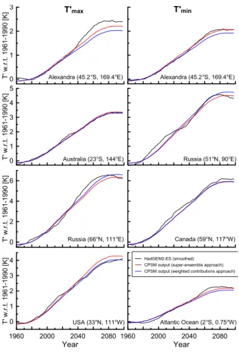
4.5 simulation was used as the predictor time series. As men-tioned in Sect. 3, in this study the focus is on exploring the methodological aspects of the pattern-scaling approach and therefore output from the same AOGCM (but different emis-sions scenario) is used in application mode instead of using time series from a SCM. By comparing time series generated by the CPSM with time series from the HadGEM2-ES RCP 4.5 simulation, a validation of the CPSM can be achieved. The Savitzky–Golay smoothedTmax′ andTmin′ annual mean time series from the raw HadGEM2-ES RCP 4.5 simulation are compared to the annual mean time series derived from the CPSM output for four selected locations and are shown in Fig. 10.
The results from the weighted contributions approach (blue line in Fig. 10) agree reasonably well with the re-sults derived from the super-ensemble approach (red line in Fig. 10) for both T′
max and T
′
min. Both the output from
!"
# $% !"
& ' !"
( ' )"
* %+!, ! - . %" /0 , 1 1 $ -2 11 3." /0 , 1 4. % 3 $ 2 $ 11 3."
/ $ % ' 5 )" & ' !"
$ 3 63 $ 5 )"
# $% !"
Fig. 10. Annual mean Tmax′ (left column) and Tmin′ (right
col-umn) time series from the HadGEM2-ES RCP 4.5 simulation (smoothed) compared to annual mean CPSM output based on the same emissions scenario using the regression model fit coefficients from the super-ensemble (Sect. 6.1) and the weighted contributions (Sect. 6.2) approaches based on RCP 2.6 and RCP 8.5 training. Note
the different scales on theyaxes.
in both the super-ensemble and weighted contribution ap-proach. Furthermore,Tmax′ warms faster than it would be ex-pected fromTglobal′ . Theα value for RCP 4.5 is effectively greater than for RCP 2.6 and RCP 8.5 (see Fig. 8) and, there-fore, when the training is performed on RCP 2.6 and RCP 8.5, the amplitude of theTmax′ signal is underestimated.
Since theTglobal′ time series from the RCP 4.5 simulation is more similar in magnitude to the RCP 2.6 simulation than the RCP 8.5 simulation, in the weighted contributions approach the fields derived from the RCP 2.6 derived fit coefficients (F′in Eq. 5) is weighted more than the fields obtained using the regression model fit coefficients derived from the RCP 8.5 simulation. In contrast, in the super-ensemble approach, the correlation between Tmax′ andTglobal′ is driven primar-ily by the strongest signal which, in this study, comes from theTmax′ time series obtained from the RCP 8.5 simulation. Therefore, if the evolution of the climate variable of interest
for RCP 2.6 emissions scenario is similar to the one from the RCP 4.5 emissions scenario, using the coefficients from the weighting contribution approach in the CPSM applica-tion will reproduce the evoluapplica-tion of the climate variable un-der RCP 4.5 better than the application of the super-ensemble coefficients (e.g. the USA site in Fig. 10). If, however, the evolution of the climate variable of interest for RCP 8.5 is similar to that from RCP 4.5, using the fit coefficients from the super-ensemble approach will reproduce the evolution of the climate variable slightly better (e.g.Tmin′ for Alexandra in Fig. 10).
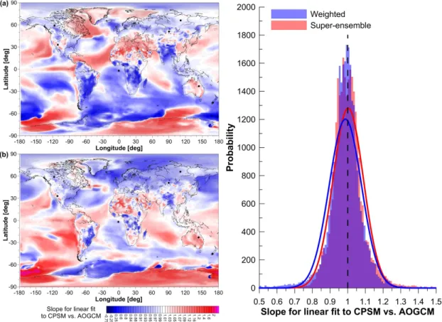
To derive a more robust and global measure of how well the CPSM (based on (a) the weighted contribution, and (b) the super-ensemble approaches) can reproduce the RCP 4.5Tmin′ time series modelled by HadGEM2-ES when trained on the RCP 2.6 and RCP 8.5 simulations, time series ofT′
min
obtained from the CPSM were regressed against smoothed time series of the same variable from the AOGCM. The slopes of linear fits to the scatter plots of CPSM data against AOGCM data from the two approaches are shown in Fig. 11 together with the probability distribution function of the slopes (histogram in the rightmost panel of Fig. 11). If the Tmin′ time series from the CPSM and from the AOGCM out-put at each grid point showed the same secular variation, all values plotted in Fig. 11 would be 1.0.
The calculated slopes using results from both methods bracket the range 0.8 to 1.2 almost everywhere, with regions in the high northern and southern latitudes exhibiting slopes that are statistically significantly different from 1.0 at the 2σ level (hatched area in Fig. 11). The probability distribu-tion funcdistribu-tions of the slopes indicate that the super-ensemble approach seems to be marginally better in reproducing the AOGCM results than the individual weighting approach; the most likely value derived from a Gaussian fit to the his-tograms is 1.006±0.0991 for the super-ensemble approach compared 0.983±0.107 for the weighted contributions ap-proach.
The results presented here do not robustly discriminate between the super-ensemble and individual weighting ap-proaches. Which of the two approaches gives better agree-ment with the AOGCM signal depends on the location, for example, in the north-east of Scandinavia the individ-ual weighting approach reproduces the AOGCM time se-ries more accurately while over India the super-ensemble ap-proach might be a better choice.
7 Time dependence of the fit coefficients
Fig. 11. The linear slopes obtained by regressingTmin′ time series from the CPSM against time series obtained from HadGEM2-ES
(smoothed) using(a)the weighted contributions approach and(b)the super-ensemble approach. Stippled regions show where the slopes
are not statistically significantly different from 1.0 at the 2σ level. Small black dots show the locations of the sites from Fig. 10. The
rightmost panel shows the PDF of the linear slopes for both the weighting contributions approach and the super-ensemble approach.
dependence on time, that is, theαkof Eq. (2) were expanded
as
αk=αk0+αk1×t, (6)
wheret represent the number of years after 1980 (t is nega-tive for years before 1980).
The regression model was then trained onTmax′ andTmin′ time series from the HadGEM2-ES RCP 4.5 simulation, whereTglobal′ was the only predictor.α was expanded first as shown in Eq. (2) and then, secondly, with each of theαk
of Eq. (2) expanded further as in Eq. (6).
As in Sect. 4.4, the SSR value was calculated for each AOGCM grid cell, where the SSR value, calculated from the model with time dependent fit coefficients, was divided by the SSR value calculated from the model where time depen-dent in the fit coefficients was excluded. The resultant ratios forTmax′ andTmin′ , usingTglobal′ from the RCP 4.5 emissions scenario as the sole predictor, are shown in Fig. 12.
Over most of the globe the inclusion of time dependence in the regression model fit coefficient reduces the sum of the squares of the residuals. Reductions are smallest over north-ern hemispheric land and Antarctic landmass with a most
common reduction of 30 % or less. Over the Weddell Sea and over the Arctic ocean, the sum of the squares of the residu-als of the regression model fit to HadGEM2-ES time series ofTmax′ andTmin′ can be reduced by up to 50 % by including time dependence in the regression model fit coefficients. The blue patches in Fig. 12 over the Pacific and Indian oceans indicate that including this time dependence can reduce the SSR by about 70 %. While including time dependence in the fit coefficients can improve the variance explained by the re-gression model, these gains are observed more over ocean than over land. We consider the gains over land to be suffi-ciently small as to not warrant including time dependence in the fit coefficients.
8 Discussion and conclusions
Fig. 12.SSRincl. time/SSRexcl. timeratios for(a)Tmax′ and(b)Tmin′ .
The ratios were derived by dividing theTmax′ (Tmin′ ) time series
from the HadGEM2-ES RCP 4.5 simulation and theTmax′ (Tmin′ )
from the regression model based on the same emissions scenarios
where (i) the time dependence was included (SSRincl. time, Eq. 6),
and (ii) time dependence was excluded (SSRexcl. time, Eq. 2).
on which it was not trained. This study has shown that this test is passed over most regions of the globe; again the Arc-tic is where it is most likely to fail. However, validating the performance of the CPSM with a single AOGCM simulation may be partially compromised by unforced variability (e.g. El Niño–Southern Oscillation, ENSO) in the AOGCM, al-though in this study we have smoothed the time series with the goal of removing such variability. Access to ensembles of simulations would be valuable in this regard. Dealing with non-linearities in the response of a local climate variable to global forcings also presents a challenge to the CPSM. Cross-scenario linearity and linearity in time-dependence of the fit coefficients were both explored. It was found that a break-down in linearity across scenarios (i.e. regression model fit coefficients are scenario dependent) occurs primarily in the Arctic. Including a linear time dependence in the regres-sion model fit coefficients improves the performance of the
CPSM, primarily over the oceans. Access to additional pre-dictor time series, such as hemispheric mean ocean and land temperatures also improves model performance, again pri-marily over the oceans. However, when more than one pre-dictor time series is used, it is essential that the prepre-dictor basis functions are orthogonalised prior to use. Where more than a single simulation are available to train the CPSM, two different approaches were explored, namely, (1) the super-ensemble approach and (2) the weighted contributions ap-proach. Our CPSM diagnostics did not provide a robust in-dication which of these two methods best reproduces the cli-mate response pattern from an AOGCM.
The RCP scenarios which formed the basis for the sim-ulations used in this study do not only differ in their long-term forcing agents (such as CO2) but also in their short-term
forcing agents (such as black carbon aerosol) and differences in the balance between short-lived and long-lived radiative forcing agents in the RCP scenarios may affect the robust-ness of the derivation of the regression model fit coefficients. The effects of such differences in short-lived radiative forc-ing agents, which act locally, and long-lived radiative forcforc-ing agents, which act globally, across the RCP scenarios has not been quantitatively assessed in this study. This might, in part, cause the non-linearity which manifests as emissions sce-nario dependence in the fit coefficients at some locations. The differing effects of short-term and long-term forcing agents on the derivation of the regression model fit coefficients will be investigated in a future study.
The scope of this study was to present a newly developed CPSM and to investigate some methodological aspects of the pattern-scaling approach. For that purpose the climate pat-terns were derived from one AOGCM only, HadGEM2-ES. In a future study we intend to apply the pattern-scaling ap-proach to a number of simulations from different AOGCMs. This will allow an estimate of the spread of sensitivities of climate variables to changes in global mean temperature due to different model parameterisations.
Appendix A
The HadGEM2-ES AOGCM
The HadGEM2-ES simulations were obtained from the World Climate Research Programme’s (WCRP’s) CMIP5 multi-model data set which is collected, organised, and archived by the Program for Climate Model Diagnostics and Intercomparison (PCMDI). Only a brief description of HadGEM2-ES is provided here since detailed documentation can be found in Collins et al. (2011) and Jones et al. (2011).
HadGEM2-ES is a coupled AOGCM with a spectral horizontal resolution of the atmospheric model component of N96, comparable to 1.875◦×1.25◦ on a transformed longitude–latitude grid. The atmospheric component of the model consists of 38 vertical layers, extending to over 39 km in altitude. The ocean component has a horizontal resolution of 1◦ (decreasing to 1/3◦ at the equator) and 40 unevenly spaced vertical levels. HadGEM2-ES includes an interac-tive land and ocean carbon cycle and an interacinterac-tive tropo-spheric chemistry scheme which simulates the evolution of atmospheric composition and interaction with atmospheric aerosols.
The HadGEM2-ES data sets used in this study consist of daily output from an historical simulation and simulations based on the following Representative Concentration Path-way (RCP) emissions scenarios (Moss et al., 2010):
– RCP 2.6 whose radiative forcing peaks at∼3 W m−2 before 2100 and then declines to stabilise at 2.6 W m−2
after 2100.
– RCP 4.5 whose radiative forcing increases monotoni-cally to 4.5 W m−2in 2100 and stabilises thereafter.
– RCP 8.5 with radiative forcing rising to 8.5 W m−2in 2100.
Monthly mean global fields ofTmaxandTminwere
calcu-lated from the daily fields, as were (up to five) globally and regionally averaged annual mean time series used as the pre-dictors. In all cases, anomalies were calculated by subtracting the 1961–1990 climatology, obtained from the historical sim-ulation, from the monthly mean fields. By using the CPSM to model only the anomalies away from the 1961–1990 base-line, an observations-based climatology can later be used to provide the baseline, thereby producing fields that are not af-fected by systematic AOGCM biases.
Mitchell (2003) showed that more statistically robust re-gression model fit coefficients can be obtained by lengthen-ing the period over which the model is fitted. Therefore the calculated monthly mean fields from the historical simula-tion (1961 to 2005) were extended with monthly mean fields from the three RCP simulations (2006 to 2100) to produce three continuous time series extending from 1961 to 2100 on which the regression model can be trained. Since the RCP
simulations were initialised using the historical simulation, a smooth transition from the historical to the future simulations is ensured.
Acknowledgements. We acknowledge the modelling groups, the Program for Climate Model Diagnosis and Intercomparison (PCMDI) and the WCRP’s Working Group on Coupled Modelling (WGCM) for their roles in making available the WCRP CMIP5 multi-model data set. For CMIP the US Department of Energy’s Program for Climate Model Diagnosis and Intercomparison provides coordinating support and led development of software infrastructure in partnership with the Global Organization for Earth System Science Portals. This work was funded under Ministry of Primary Industries contract CX09X1004 and, in part, under the Ministry of Business, Innovation and Employment contract C01X1225.
Edited by: J. Annan
References
Bodeker, G. E., Boyd, I. S., and Matthews, W. A.: Trends and vari-ability in vertical ozone and temperature profiles measured by ozonesondes at Lauder, New Zealand: 1986–1996, J. Geophys. Res., 103, 28661–28681, 1998.
Collins, W. J., Bellouin, N., Doutriaux-Boucher, M., Gedney, N., Halloran, P., Hinton, T., Hughes, J., Jones, C. D., Joshi, M., Lid-dicoat, S., Martin, G., O’Connor, F., Rae, J., Senior, C., Sitch, S., Totterdell, I., Wiltshire, A., and Woodward, S.: Develop-ment and evaluation of an Earth-System model – HadGEM2, Geosci. Model Dev., 4, 1051–1075, doi:10.5194/gmd-4-1051-2011, 2011.
Frieler, K., Meinshausen, M., Mengel, M., Braun, N., and Hare, W.: A Scaling Approach to Probabilistic Assessment of Regional Cli-mate Change, J. CliCli-mate, 25, 3117–3144, 2012.
Giorgi, F.: Interdecadal variability of regional climate change: im-plications for the development of regional climate change sce-narios, Meteorol. Atmos. Phys., 89, 1–15, 2005.
Huntingford, C. and Cox, P.M.: An analogue model to derive addi-tional climate change scenaios from exisiting GCM simulations, Clim. Dynam., 16, 575–586, 2000.
Jones, C. D., Hughes, J. K., Bellouin, N., Hardiman, S. C., Jones, G. S., Knight, J., Liddicoat, S., O’Connor, F. M., Andres, R. J., Bell, C., Boo, K.-O., Bozzo, A., Butchart, N., Cadule, P., Corbin, K. D., Doutriaux-Boucher, M., Friedlingstein, P., Gor-nall, J., Gray, L., Halloran, P. R., Hurtt, G., Ingram, W. J., Lamar-que, J.-F., Law, R. M., Meinshausen, M., Osprey, S., Palin, E. J., Parsons Chini, L., Raddatz, T., Sanderson, M. G., Sellar, A. A., Schurer, A., Valdes, P., Wood, N., Woodward, S., Yoshioka, M., and Zerroukat, M.: The HadGEM2-ES implementation of CMIP5 centennial simulations, Geosci. Model Dev., 4, 543–570, doi:10.5194/gmd-4-543-2011, 2011.
Meinshausen, M., Meinshausen, N., Hare, W., Raper, S. C. B., Frieler, K., Knutti, R., Frame, D. J., and Allen, M. R.: Greenhouse-gas emission targets for limiting global warming to 2oC, Nature, 458, 1158–1162, 2009.
ibration, Atmos. Chem. Phys., 11, 1417–1456, doi:10.5194/acp-11-1417-2011, 2011.
Mitchell, J. F. B., Johns, T. C., Eagles, M., Ingram, W. J., and Davis, R. A.: Towards the construction of climate change scenarios, Cli-matic Change, 41, 547–581, 1999.
Mitchell, T. D.: Pattern scaling: An Examination of the Accuracy of the Technique for Describing Future Climates, Climatic Change, 60, 217–242, 2003.
Mitchell, T. D. and Jones, P. D.: An improved method of construct-ing a database of monthly climate observations and associated high-resolution grids. Int. J. Climatol., 25, 693–712, 2005. Moritz, R. E., Bitz, C. M., and Steig, E. J.: Dynamics of recent
climate change in the Arctic, Science, 297, 1497–1502, 2002. Moss, R. H., Edmonds, J. A., Hibbard, K. A., Manning, M. R., Rose,
S. K., van Vuuren, D. P., Carter, T. R., Emori, S., Kainuma, M., Kram, T., Meehl, G. A., Mitchell, J. F. B., Nakicenovic, N., Riahi, K., Smith, S. J., Stouffer, R. J., Thomson, A. M., Weyant, J. P., and Wilbanks, T. J.: The next generation of scenarios for climate change research and assessment, Nature, 463, 747–756, 2010. Parry, M. L., Canziani, O. F., Palutikof, J. P., van der Linden, P. J.,
and Hanson, C. E. (Eds.): Climate Change 2007: Impacts, Adap-tation and Vulnerability, Contribution of Working Group II to the Fourth Assessment Report of the Intergovernmental Panel on Climate Change, Cambridge University Press, 976 pp., 2007. Press, W. H., Flannery, B. R., Teukolsky, S. A., and Vettering, W.
T.: Numerical Recipes in Pascal, Cambridge University Press, 759 pp., 1989.
mean total ozone and lower stratospheric temperature, J. Geo-phys. Res., 99, 5433–5447, 1994.
Reinsel, G. C., Miller, A. J., Weatherhead, E. C., Flynn, L. E., Na-gatani, R. M., Tiao, G. C., and Wuebbles, D. J.: Trend analysis of total ozone data for turnaround and dynamical contributions, J. Geophys. Res., 110, D16306, doi:10.1029/2004JD004662, 2005. Ruosteenoja, K., Tuomenvirta, H., and Jylhä, K.: GCM-based re-gional temperature and precipitation change estimates for Europe under four SRES scenarios applying a super-ensemble pattern-scaling method, Climatic Change, 81, 193–208, 2007.
Savitzky, A. and Golay, M. J. E.: Smoothing and differentiation of data by simplified least squares procedures, Vol. 36, 1964. Serreze, M. C. and Barry, R. G.: Processes and impacts of Arctic
amplification: A research synthesis, Global Planet. Change, 77, 85–96, 2011.
Tiao, G. C., Reinsel, G. C., Xu, D., Pedrick, J. H., Zhu, X., Miller, A. J., DeLuisi, J. J., Mateer, C. L., and Wuebbles, D. J.: Effects of autocorrelation and temporal sampling schemes on estimates of trend and spatial correlation, J. Geophys. Res., 95D12, 20507– 20517, 1990.