Export Performance and Economic Growth in
East Asian Economies
–
Application of
Cointegration and Vector Error Correction
Model
Neena MALHOTRA
*, Deepika KUMARI
**Abstract
East Asian Economies are considered to be most successful economies in the world. Following the footsteps of other East Asian economies such as Japan and South Korea, China also shifted towards export-led growth strategy in 80s. This study analyzes the effect of export performance on economic growth of three major East Asian economies i.e. Japan, South Korea, and China. This study has conducted the econometric analysis of macro data under multivariate framework for the period 1980-2012. In order to examine the causal relationship between exports and economic growth, the study has applied time series techniques such as Augmented Dickey-Fuller (ADF) and Phillips-Perron (PP) unit root tests to check stationarity of variables, Johansen cointegration test for long run relationship, vector error correction model (VECM) for short run dynamics and for estimating speed of adjustment towards long run equilibrium. The analysis also made use of techniques Impulse Response Function (IRF) and Variance Decomposition Analysis (VDA) to investigate the interrelationships within the system. The estimated results suggested that all variables were cointegrated for East Asian economies. The study concluded that export-led growth (ELG) was only long run phenomenon in China and South Korea. The results for Japan supported growth led exports (GLE) particularly for short run.
Keywords: Export-led Growth, Southeast Asia, time series, cointegration, VECM, impulse response function, variance decomposition analysis
JEL Code Classification: C12, C32, F14, F43 UDC: 339.564(5-12):330.35
DOI: https://doi.org/10.17015/ejbe.2016.018.08
*
Corresponding author. Associate Professor, Punjab School of Economics, Guru Nanak Dev University, Punjab, India. E-mail: [email protected].
**
1.
Introduction and Background
After Second World War, Japan focused on industrialization and expansion of exports which led to rapid economic growth of the e o o . Later o , Japa s export-led growth model was adopted by four Asian tigers or first tier of newly industrialized economies (NIEs) namely Hong Kong, South Korea, Singapore and Taiwan in the 1960s. After the success of four Asian tigers since 1970, second tier of newly industrialized economies (NIEs) of Southeast Asia namely Indonesia, Malaysia, Thailand and Philippines replicated this strategy. Finally China and India gradually followed this strategy. Hence, rapidly growing economies of Asian region have widely followed export-led growth strategy as an effective tool for development (Page, 1994; Kokko, 2002; Chow, 2012).
East Asia is considered as most successful sub region of Asia. China is the largest country in terms of geographic and demographic features. Chi a s populatio is te
ti es ore tha Japa s populatio a d t e t se e ti es that of South Korea.
Japan and South Korea are located just off the coast of mainland China. In 2012, China, Japan and South Korea together constituted about 20 percent of world economic output in nominal terms. Moreover, China was also the largest trading partner of both Japan and South Korea in the same year. Industrialization was the main reason behind the economic development of these economies (Berglee, 2012; O ‘eill , ; Park & Patrick, 2013).
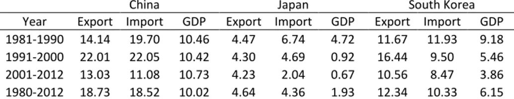
The compound growth rates of exports, imports and trade for East Asian economies have been reported in Table 1. Table indicates remarkable exports performance of China and South Korea during 1981-2012. However, Japa s e port performance was low during 80s and further declined during later decades. In case of GDP, only China was able to secure double digit growth throughout the study period. Growth rates of exports and GDP are relatively lower for Japan, which is due to Japan being a mature developed economy as well as slowdown in developed world.
Table 1. Growth performance of East Asian Economies (Compound
Growth Rates)
China Japan South Korea
Year Export Import GDP Export Import GDP Export Import GDP 1981-1990 14.14 19.70 10.46 4.47 6.74 4.72 11.67 11.93 9.18 1991-2000 22.01 22.05 10.42 4.30 4.69 0.92 16.44 9.50 5.46 2001-2012 13.03 11.08 10.73 4.23 2.04 0.67 10.56 8.47 3.86 1980-2012 18.73 18.52 10.02 4.64 4.36 1.93 12.34 10.33 6.15
Source: Calculations based on data from World Development Indicators (WDI), online database.
includes structural breaks, diagnostic tests and forecasting methods such as impulse response function (IRF) and variance decomposition analysis (VDA). The first section includes introductory part and brief background of East Asian economies. The next section reports review of literature. Further, methodology and empirical results have been given. Final section presents conclusions and also contains comparison of our results with previous studies.
2.
Review of Literature
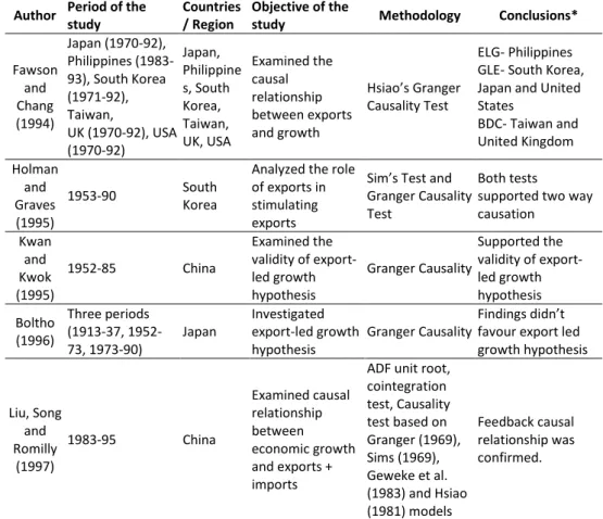
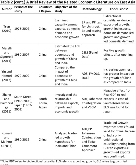
The literature reviewed indicates that comprehensive studies based on rigorous statistical analysis comprising forecasting methods and identifying structural breaks are lacking (Table 2). Therefore, the present study has made an attempt to analyze the relationship between exports and economic growth by adopting above mentioned methods. The evidence for export-led growth hypothesis is inconclusive as the results provided by these studies are not unanimous. Hence, in the light of above facts, the study takes into account these issues in further investigation.
Table 2. A Brief Review of the Related Economic Literature on East Asia
Author Period of the study
Countries / Region
Objective of the
study Methodology Conclusions*
Fawson and Chang (1994)
Japan (1970-92), Philippines (1983-93), South Korea (1971-92), Taiwan,
UK (1970-92), USA (1970-92)
Japan, Philippine s, South Korea, Taiwan, UK, USA
Examined the causal relationship between exports and growth
Hsiao s Granger Causality Test
ELG- Philippines GLE- South Korea, Japan and United States
BDC- Taiwan and United Kingdom
Holman and Graves (1995)
1953-90 South Korea
Analyzed the role of exports in stimulating exports
Si s Test a d
Granger Causality Test
Both tests
supported two way causation
Kwan and Kwok (1995)
1952-85 China
Examined the validity of export-led growth hypothesis
Granger Causality
Supported the validity of export-led growth hypothesis
Boltho (1996)
Three periods (1913-37, 1952-73, 1973-90)
Japan
Investigated export-led growth hypothesis
Granger Causality
Fi di gs did t
favour export led growth hypothesis
Liu, Song and Romilly
(1997)
1983-95 China
Examined causal relationship between economic growth and exports + imports
ADF unit root, cointegration test, Causality test based on Granger (1969), Sims (1969), Geweke et al. (1983) and Hsiao (1981) models
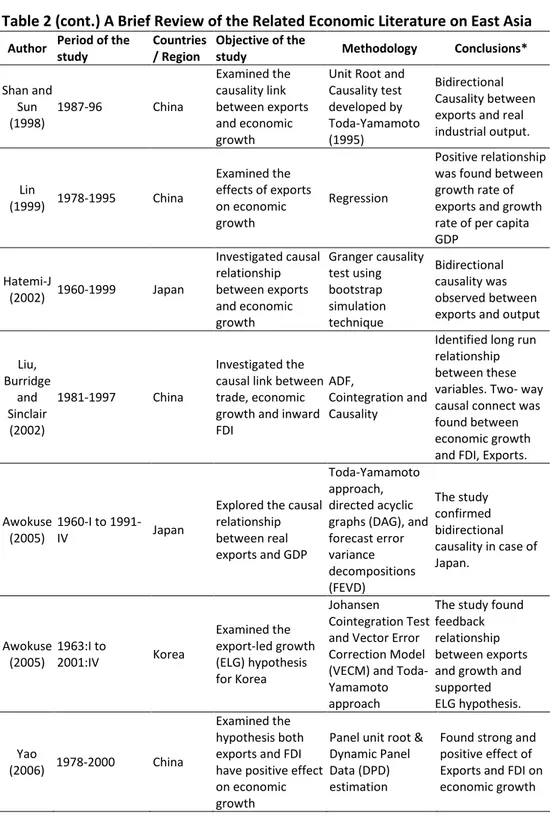
Table 2 (cont.) A Brief Review of the Related Economic Literature on East Asia
Author Period of the study
Countries / Region
Objective of the
study Methodology Conclusions*
Shan and Sun (1998)
1987-96 China
Examined the causality link between exports and economic growth
Unit Root and Causality test developed by Toda-Yamamoto (1995)
Bidirectional Causality between exports and real industrial output.
Lin
(1999) 1978-1995 China
Examined the effects of exports on economic growth
Regression
Positive relationship was found between growth rate of exports and growth rate of per capita GDP
Hatemi-J
(2002) 1960-1999 Japan
Investigated causal relationship between exports and economic growth
Granger causality test using bootstrap simulation technique
Bidirectional causality was observed between exports and output
Liu, Burridge
and Sinclair (2002)
1981-1997 China
Investigated the causal link between trade, economic growth and inward FDI
ADF,
Cointegration and Causality
Identified long run relationship between these variables. Two- way causal connect was found between economic growth and FDI, Exports.
Awokuse (2005)
1960-I to
1991-IV Japan
Explored the causal relationship between real exports and GDP
Toda-Yamamoto approach, directed acyclic graphs (DAG), and forecast error variance decompositions (FEVD)
The study confirmed bidirectional causality in case of Japan.
Awokuse (2005)
1963:I to
2001:IV Korea
Examined the export-led growth (ELG) hypothesis for Korea
Johansen Cointegration Test and Vector Error Correction Model (VECM) and Toda-Yamamoto approach
The study found feedback relationship between exports and growth and supported ELG hypothesis.
Yao
(2006) 1978-2000 China
Examined the hypothesis both exports and FDI have positive effect on economic growth
Panel unit root & Dynamic Panel Data (DPD) estimation
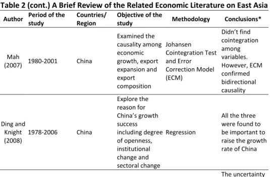
Table 2 (cont.) A Brief Review of the Related Economic Literature on East Asia
Author Period of the study
Countries/ Region
Objective of the
study Methodology Conclusions*
Mah
(2007) 1980-2001 China
Examined the causality among economic growth, export expansion and export composition
Johansen Cointegration Test and Error Correction Model (ECM)
Did t fi d
cointegration among variables. However, ECM confirmed bidirectional causality
Ding and Knight (2008)
1978-2006 China
Explore the reason for
Chi a s gro th
success including degree of openness, institutional change and sectoral change
Regression
All the three were found to be important to raise the growth rate of China
Mahade van and Suardi (2008)
Up to 2005 (more than 30 years)
Japan, Korea, Taiwan & Hong-Kong
Examined the stability of trade-growth nexus by incorporating the effects of uncertainty or volatility
ADF, KPSS tests for unit root,
Cointegration, VECM
The uncertainty results revealed GDP growth was import led in Japan, both export & import led in Hong-Kong, mutually causative in Taiwan. No causation from GDP growth to exports and imports was observed for Korea (vice versa). Herreria
s and Orts (2010)
1964-2004 China
Analyzed whether growth is export- led or investment- led
ADF, VECM Found evidence for both
Sun and Heshmat i (2010)
2002-2007 China
Evaluated the effect of international trade on economic growth
Likelihood Ratio Test, One Way ANOVA, Non Parametric Test
Table 2 (cont.) A Brief Review of the Related Economic Literature on East Asia
Author Period of the study
Countries / Region
Objective of the
study Methodology Conclusions*
Tsen
(2010) 1978-2002 China
Examined causality among exports, domestic demand and economic growth
ER and PP test for Unit root, Bound testing approach
Bidirectional causality, evidence of export-led growth, growth led exports, domestic demand led growth and growth led domestic demand
Marelli and Signorelli
(2011)
1980-2007 China
Estimated the link between
openness and growth of China and India
2SLS (Panel Data)
Positive growth effects after opening up.
Yin and Hamori (2012)
1970-2009 China
Compared the impact of openness on growth of China and India
ADF, FMOLS, DOLS
Increasing openness has greater impact on the growth of China as compare to India
Zhang and Baimbrid
ge (2011)
South Korea (1963-2003), Japan (1957-2003)
South Korea, Japan
Investigated the relationship between exports, imports and economic growth
ADF, Johansen Cointegration and VECM
Negative effect from Real GDP to real exports in case of South Korea while ELG was found for Japan
Kumari and Malhotr a (2014)
1980-2012 China
Analyzed trade-led growth hypothesis for India and China
ADF,PP, Johansen Cointegration and Toda-Yamamoto Approach
Trade-led Growth hypothesis was found valid for China. In case of India only
unidirectional causality running from GDP to exports i.e. growth-led exports was confirmed.
*Note: BDC refers to bi-directional causality, ELG refers to export led growth, GLE refers to growth led export.
3.
Model, Database and Econometric Strategy
The aggregate production function used in the study can be expressed as:
Y= f (K, L, X, M) (1)
export-led growth (ELG) hypothesis for major East Asian economies. The study has used annual data at the 2005 constant US dollar prices from 1980 to 2012. Data on real GDP per capita(GDPPC), real exports(EXP), real imports(IMP), real gross capital formation(GCF) has been compiled from World Development Indicators (WDI) online database, World Bank, while data on total labour force(LAB) is collected from United Nation Conference on Trade and Development (UNCTAD) Statistics.
All the variables are taken in their natural logarithms to avoid the problem of heteroskedasticity (Gujarati 1995).For the application of multivariate econometric techniques, the above stated model can be expressed in the following linear logarithmic form:
= + + + + +
The prefi LN sta ds for atural logarith . The stud takes i to a ou t du ies
for Asian Financial Crisis (1997) and Global Economic Crisis (2008). To examine the export-led growth hypothesis cointegration and VECM based causality tests have been used.
4.
Estimates of Multivariate Analysis
4.1.
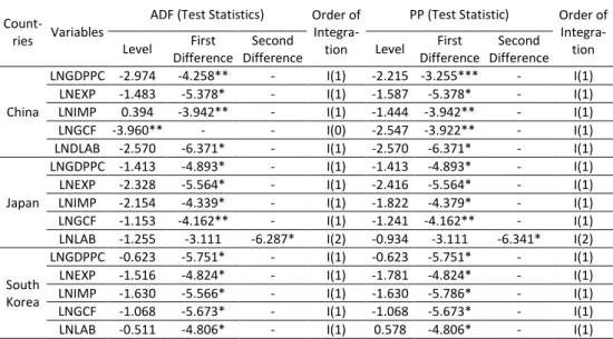
Unit Root Results
The results in Table 3 give the summary of ADF and PP tests for East Asian economies.
Table 3. Results of Unit Root test for variables
Count-ries Variables
ADF (Test Statistics) Order of
Integra-tion
PP (Test Statistic) Order of
Integra-tion Level First
Difference
Second
Difference Level
First Difference
Second Difference
China
LNGDPPC -2.974 -4.258** - I(1) -2.215 -3.255*** - I(1)
LNEXP -1.483 -5.378* - I(1) -1.587 -5.378* - I(1)
LNIMP 0.394 -3.942** - I(1) -1.444 -3.942** - I(1)
LNGCF -3.960** - - I(0) -2.547 -3.922** - I(1)
LNDLAB -2.570 -6.371* - I(1) -2.570 -6.371* - I(1)
Japan
LNGDPPC -1.413 -4.893* - I(1) -1.413 -4.893* - I(1)
LNEXP -2.328 -5.564* - I(1) -2.416 -5.564* - I(1)
LNIMP -2.154 -4.339* - I(1) -1.822 -4.379* - I(1)
LNGCF -1.153 -4.162** - I(1) -1.241 -4.162** - I(1)
LNLAB -1.255 -3.111 -6.287* I(2) -0.934 -3.111 -6.341* I(2)
South Korea
LNGDPPC -0.623 -5.751* - I(1) -0.623 -5.751* - I(1)
LNEXP -1.516 -4.824* - I(1) -1.781 -4.824* - I(1)
LNIMP -1.630 -5.566* - I(1) -1.630 -5.786* - I(1)
LNGCF -1.068 -5.673* - I(1) -1.068 -5.673* - I(1)
LNLAB -0.511 -4.806* - I(1) 0.578 -4.806* - I(1)
Augmented Dickey- Fuller (ADF) test and Phillip-Perron (PP) test (including constant with trend) for five variables namely LNGDPPC, LNEXP, LNIMP, LNGCF &LNLAB have been applied to check whether series are stationary or not. The results revealed the presence of unit root for all series at levels. After differencing, all series were found to be stationary except the series LNLAB for Japan. The variable integrated of order two or I(2) was dropped from the model in case of Japan.
4.2.
Chow Test Results
Time series plotting of the variables indicated the presence of structural breaks. Hence, Chow breakpoint test has been used to identify and confirm structural break in dataset. This test analyzes the null hypothesis of no structural break.
The results in Table 4 clearly indicate the absence of structural break in dataset as
the ull h pothesis of o stru tural reak a t e reje ted for Chi a. For Japa a d
South Korea, the results affirmed the presence of structural break in dataset. Asian
risis of had se ere i pa t o South Korea s e o o . The results sho ed the prese e of stru tural reak for Japa a d South Korea s dataset for .
Table 4. Results of Chow Breakpoint Test
China
Chow Breakpoint Test: 2008
Null Hypothesis: No breaks at specified breakpoints Equation Sample: 1981 2012
F-statistic 0.230 Prob.F 0.945
Log likelihood ratio 1.634 Prob. Chi-Square 0.897 Wald Statistic 1.152 Prob. Chi-Square 0.949
Japan
Chow Breakpoint Test: 2008
Null Hypothesis: No breaks at specified breakpoints Equation Sample: 1981 2012
F-statistic 2.460 Prob.F 0.064
Log likelihood ratio 14.212 Prob. Chi-Square 0.014 Wald Statistic 12.300 Prob. Chi-Square 0.030
South Korea
Chow Breakpoint Test: 1997 & 2008
Null Hypothesis: No breaks at specified breakpoints Equation Sample: 1981 2012
F-statistic 10.408 Prob.F 0.000
Log likelihood ratio 39.023 Prob. Chi-Square 0.000 Wald Statistic 52.040 Prob. Chi-Square 0.000
F-statistic 4.637 Prob.F 0.004
4.3.
VAR Lag Order Selection Criteria
The next step involves investigation of the long run relationship among variables. Before applying Johansen cointegration procedure appropriate lag length must be set. In Table 5, the results of VAR lag order selection criteria have been presented. Schwarz information criterion was adopted to estimate cointegration and unrestricted VAR.
Table 5. Results of VAR Lag Order Selection Criteria
China
Endogenous variables: LNGDPPC LNEXP LNIMP LNGCF LNDLAB Exogenous variables: C Sample: 1980 2012
Lag LR FPE AIC SC HQ
0 NA 2.21e-08 -3.440 -3.204 -3.366
1 235.495 4.56e-12 -11.955 -10.541* -11.512 2 40.505* 3.19e-12 -12.481 -9.888 -11.669 3 35.946 1.84e-12* -13.522* -9.750 -12.341*
Japan
Endogenous variables: LNGDPPC LNEXP LNIMP LNGCF Exogenous variables: C DUMMY Sample: 1980 2012
Lag LR FPE AIC SC HQ
0 NA 1.51e-08 -6.656 -6.467 -6.596
1 249.127 1.43e-12 -15.932 -14.989* -15.637 2 27.590* 1.17e-12* -16.208* -14.511 -15.677* 3 9.649 2.33e-12 -15.708 -13.256 -14.940 4 16.891 2.59e-12 -16.012 -12.806 -15.008
South Korea
Endogenous variables: LNGDPPC LNEXP LNIMP LNGCF LNLAB Exogenous variables: C DUMMY1 DUMMY2 Sample: 1980 2012
Lag LR FPE AIC SC HQ
0 NA 1.09e-13 -15.659 -14.959 -15.435
1 192.166 9.90e-17 -22.727 -20.859* -22.130 2 38.459* 6.94e-17 -23.323 -20.287 -22.352 3 27.603 6.88e-17* -23.957* -19.753 -22.612*
* indicates lag order selected by the criterion
LR: sequential modified LR test statistic (each test at 5% level) FPE: Final prediction error
AIC: Akaike information criterion SC: Schwarz information criterion HQ: Hannan-Quinn information criterion
4.4.
Cointegration Results
e n a M A LH O T R A & De e p ika KU MA R I g e | 144 E JB E 2016, 9 ( 18 )
Table 6. Johansen Co-integration Test Statistics for the variables
Unrestricted Cointegration Rank Test (Maximum Eigenvalue) Prob.** 0.008 0.230 0.379 0.601 0.444 0.019 0.036 0.326 0.158 0.000 0.024 0.096 0.075 0.249
Note: * indicate significance at the 5% level respectively
Critical Value 0.05 38.331 32.118 25.823 19.387 12.517 27.584 21.131 14.264 3.841 38.331 32.118 25.823 19.387 12.517 Trace 44.425 26.024 17.970 10.162 6.124 30.624 22.073 8.537 1.990 55.065 34.525 23.554 18.117 8.025 Eigen value 0.772 0.579 0.450 0.287 0.184 0.627 0.509 0.240 0.062 0.830 0.671 0.532 0.442 0.228 Hypothesized
No. of CE(s)
None *
At most 1
At most 2
At most 3
At most 4
None *
At most 1 *
At most 2
At most 3
None *
At most 1 *
At most 2
At most 3
At most 4 Unrestricted Cointegration Rank Test (Trace)
Prob.** 0.002 0.096 0.276 0.469 0.444 0.001 0.023 0.242 0.158 0.000 0.000 0.009 0.046 0.249 Critical Value 0.05 88.803 63.876 42.915 25.872 12.517 47.856 29.797 15.494 3.841 88.803 63.876 42.915 25.872 12.517 Trace 104.707 60.281 34.256 16.286 6.124 63.226 32.601 10.528 1.990 139.287 84.222 49.696 26.142 8.025 Eigen value 0.772 0.579 0.450 0.287 0.184 0.627 0.509 0.240 0.062 0.830 0.671 0.532 0.442 0.228 Hypothesized
No. of CE(s)
None *
At most 1
At most 2
At most 3
At most 4
None *
At most 1 *
At most 2
At most 3
None *
At most 1 *
At most 2 *
At most 3 *
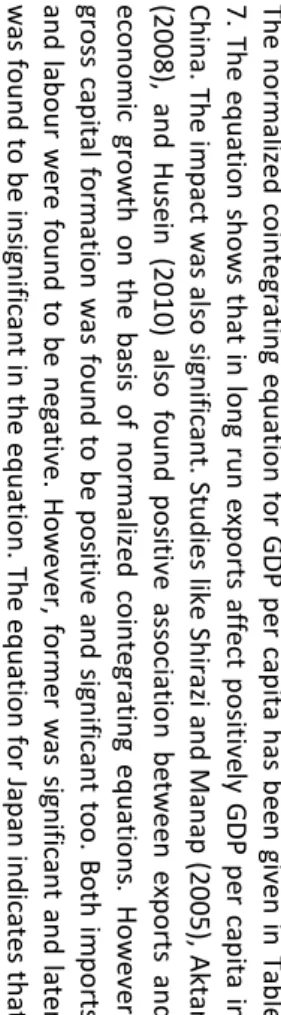
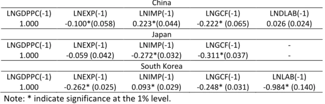
imports growth and gross capital formation have positive and significant effect on GDPPC. Although the variable exports hold positive sign but it was found to be insignificant. For South Korea, the normalized cointegrating equation indicated that in the long run all variables except imports have positive and significant impact on GDPPC.
Table 7. Normalized Cointegrating Coefficients for GDPPC Equation
China
LNGDPPC(-1) LNEXP(-1) LNIMP(-1) LNGCF(-1) LNDLAB(-1) 1.000 -0.100*(0.058) 0.223*(0.044) -0.222* (0.065) 0.026 (0.024)
Japan
LNGDPPC(-1) LNEXP(-1) LNIMP(-1) LNGCF(-1) - 1.000 -0.059 (0.042) -0.272*(0.032) -0.311*(0.037) -
South Korea
LNGDPPC(-1) LNEXP(-1) LNIMP(-1) LNGCF(-1) LNLAB(-1) 1.000 -0.262* (0.025) 0.093* (0.029) -0.248* (0.031) -0.984* (0.140) Note: * indicate significance at the 1% level.
4.5.
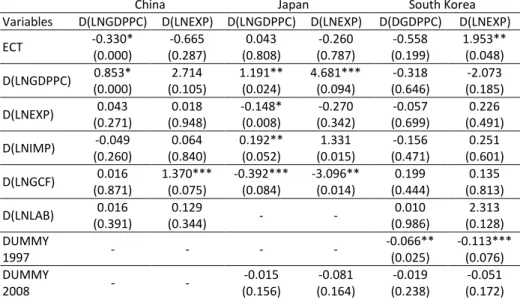
VECM Short Run Causality Results
VECM results comprise the estimate of the speed of adjustment coefficients and short run properties of series. Table 8 reports the short run causality results obtained from VECM. For China, the coefficients of error correction terms (ECT) with GDPPC and exports as dependent variable were negative but former was statistically significant at 5% level of significance indicating there is convergence from short dynamics towards long run equilibrium. The adjustment coefficient was found to be 0.33 percent implying that speed of adjustment was 33 percent towards long run equilibrium in case of disequilibrium situation. However, short run coefficients of first difference of LNEXP lagged one period for GDP per capita as dependent variable and first difference of LNGDPPC lagged one period for exports equation were found to be statistically insignificant which indicates the absence of short run causality in any direction.
In case of Japan, the results exhibit that coefficient of error correction term (ECT) was not significant in any of two cases for GDPPC and exports. However, the sign was negative (correct) for exports equation. Further, short run coefficient of first difference of LNGDPPC lagged one period for exports equation was found to be positively significant which indicated unidirectional short run causality from GDPPC to exports or growth led exports. The short run coefficient of first difference of LNEXP lagged one period for GDPPC equation was found to be negatively significant. Dummy variable was found to be negative in both cases.
towards long run equilibrium in any disequilibrium situation. Further, short run coefficients of first difference of LNEXP lagged one period for GDPPC equation and first difference of LNGDPPC lagged one period for export equation were negative and insignificant.
Table 8. Short Run Causality Results VECM
China Japan South Korea
Variables D(LNGDPPC) D(LNEXP) D(LNGDPPC) D(LNEXP) D(DGDPPC) D(LNEXP)
ECT -0.330* (0.000)
-0.665 (0.287)
0.043 (0.808)
-0.260 (0.787)
-0.558 (0.199)
1.953** (0.048)
D(LNGDPPC) 0.853* (0.000)
2.714 (0.105)
1.191** (0.024)
4.681*** (0.094)
-0.318 (0.646)
-2.073 (0.185)
D(LNEXP) 0.043 (0.271)
0.018 (0.948)
-0.148* (0.008)
-0.270 (0.342)
-0.057 (0.699)
0.226 (0.491)
D(LNIMP) -0.049 (0.260)
0.064 (0.840)
0.192** (0.052)
1.331 (0.015)
-0.156 (0.471)
0.251 (0.601)
D(LNGCF) 0.016 (0.871)
1.370*** (0.075)
-0.392*** (0.084)
-3.096** (0.014)
0.199 (0.444)
0.135 (0.813)
D(LNLAB) 0.016 (0.391)
0.129
(0.344) - -
0.010 (0.986)
2.313 (0.128) DUMMY
1997 - - - -
-0.066** (0.025)
-0.113*** (0.076) DUMMY
2008 - -
-0.015 (0.156)
-0.081 (0.164)
-0.019 (0.238)
-0.051 (0.172)
Note: *, ** and *** indicate significance at the 1%, 5% and 10% level respectively.
Thus, the results indicated the absence of short run causality between these two variables. Thus results are similar to those reported in the study by Lawrence and Weinstein (1999). Dummy variable for Asian crisis 1997 was found to be negative and statistically significant implying the negative impact of crisis on Korean economy. However, dummy variable for Global crisis 2008 was also found to be negative but statistically insignificant.
Table 9. Summary of Results
Country Cointegration Results
VECM Results (For Short Run Causality)
Impact of Dummies
China Cointegrated No short run causality -
Japan Cointegrated GLE Significant
South Korea Cointegrated No short run causality Significant
4.6.
Diagnostic Tests
that deviation from normality in case of parametric tests is not very sensitive. Wooldridge (2012) pointed out that non- normality of errors is not a serious problem with large sample size. Ghasemi and Zahediasl (2012) also suggested that with large enough sample sizes (> 30 or 40), the violation of the normality assumption should not cause major problems this implies that we can use parametric procedures even when the data are not normally distributed.
Table 10. Results of Diagnostic Tests
China Japan South Korea
Jarque-Bera Normality Test 5.870(0.053) 0.312(0.855) 45.049(0.000) ARCH Heteroskedasticity Test 0.030(0.861) 0.290 (0.589) 0.032(0.857) Breusch-Godfrey LM test 0.498(0.480) 2.184 (0.139) 02.129(0.144) Note: p-values are reported in parentheses.
4.7.
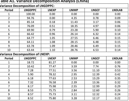
Impulse response function and variance decomposition analysis results
5.
Conclusion and Policy Implications
In order to observe the relationship between exports and economic growth for East Asian economies during 1980-2012, this study constructed multivariate framework using the variables GDP per capita, exports, imports, gross capital formation and labour. Time series techniques such as Augmented Dickey-Fuller (ADF) and Phillips-Perron (PP) unit root tests, Johansen cointegration test, vector error correction model (VECM) were employed. The analysis also made use of forecasting techniques namely Impulse Response Function (IRF) and Variance Decomposition Analysis (VDA). The study also conducts diagnostic tests for normality, heteroskedasticity, autocorrelation using Jarque-Bera Normality test, ARCH Heteroskedasticity test and Breusch-Godfrey LM test.
The estimated results suggested that all variables were cointegrated for East Asian economies. The normalized equation shows that in long run exports affects positively GDP per capita in China and South Korea. The impact was also significant. The result exhibits that coefficient of error correction term (ECT) for GDPPC equation was significant only for China indicating significant adjustments towards long run equilibrium in any disequilibrium situation. No short run causality was found between GDPPC and exports in case of China. The short run coefficient of first difference of LNGDPPC lagged one period for exports equation was found to be positively significant for Japan. In case of South Korea, the results indicated the absence of short run causality between these two variables. Hence, export-led growth (ELG) hypothesis was not found valid for China, Japan and South Korea particularly in short run however, reverse causation i.e. growth led exports (GLE) was confirmed for Japan in short run. Thus, the study concluded that export-led growth (ELG) was only long run phenomenon in China and South Korea. The results for Japan supported growth led exports (GLE) particularly for short run. Although East Asian economies export performance remained exceptionally well. But the Asian Financial Crisis 1997 and Global Economic Crisis 2008 resulted in long term adverse effects excluding China.
The results of the study clearly highlight the importance of exports in the selected East Asian economies. In the long run exports are positively affecting GDP per capita in China and South Korea. Hence, these economies should continue to promote their exports. Japan is matured developed economy with high per capita income and has different structure of the economy. Japan has experienced growth led exports in short run and hence this economy will have to promote growth internally as it is suffering from past two decades of stagnation.
Baimbridge (2011) for causality results. The study partially supported Awokuse (2005) for cointegration results while it contradicts causality results given by Fawson and Chang (1994) and Holman and Graves (1995).
References
Afzal, M., & I. Hussain (2010). Export-led Growth Hypothesis: Evidence from Pakistan. Journal of Quantitative Economics, 8(1), 130-147.
Aktar, S. T. İ. . A E piri al E a i atio of the E port-led Growth Hypothesis in Turkey. Journal of Yaşar University, 3(11), 1535-1551.
Awokuse, T. O. (2005). Export-led growth and the Japanese Economy: Evidence from VAR and Directed Acyclic Graphs. Applied Economics Letters, 12(14), 849-858. https://doi.org/10.1080/13504850500358801
Awokuse, T. O. (2005). Exports, Economic Growth and Causality in Korea. Applied Economics Letters, 12(11), 693-696. https://doi.org/10.1080/13504850500188265
Berglee, R (2012). World Regional Geography: People, Places and Globalization. Retrieved from: https://saylordotorg.github.io/text_world-regional-geography-people-places-and-globalization/index.html
Boltho, A. (1996). Was Japanese Growth Export-led?. Oxford Economic Papers, 48(3), 415-432. https://doi.org/10.1093/oxfordjournals.oep.a028576
Chow, P. C. (2012). Trade and Industrial Development in East Asia: Catching up or Falling Behind.Edward Elgar Publishing. https://doi.org/10.4337/9781849804837
Ding, S., & J. Knight (2008). Why has China Grown so Fast? The Role of Structural Change. Department of Economics Discussion Paper Series 415, University of Oxford, 1-65.
Engle, R. F., & Granger, C. W. (1987). Co-integration and Error Correction: Representation, Estimation, and Testing. Econometrica: Journal of the Econometric Society, 251-276. https://doi.org/10.2307/1913236
Evans, O. (2013). Testing Finance-Led, Export-Led and Import-Led Growth Hypotheses on Four Sub-Saharan African Economies .MPRA Paper No. 52460, University Library of Munich, Germany.
Eviews. (2006).E ie s User s Guide II , ©1994-2007 Quantitative Micro Software.
Fawson, C., & Chang, T. (1994). Cointegration, Causality, Error-Correction, and Export-Led growth in Six Countries: Japan, Philippines, South Korea, Taiwan, United Kingdom and United States. Economics Research Institute Study Paper, 94(9), 1.
Ghasemi, A., & Zahediasl, S. (2012). Normality tests for statistical analysis: a guide for non-statisticians. International journal of endocrinology and metabolism, 10(2), 486-489. https://doi.org/10.5812/ijem.3505
Gujarati, D.N. (1995).Basic Econometrics (3rd ed.), New York, Tata McGraw-Hill.
Hatemi-J, A. (2002). Export Performance and Economic Growth Nexus in Japan: A Bootstrap Approach. Japan and the World Economy, 14(1), 25-33.
Herrerias, M. J., & Orts, V. (2010). Is the Export-led Growth Hypothesis Enough to Account
for Chi a s Gro th, China & World Economy, 18(4), 34-51. https://doi.org/10.1111/j.1749-124X.2010.01203.x
Husein, J. (2010). Export-Led Growth Hypothesis in the MENA Region: A Multivariate Cointegration, Causality and Stability Analysis. Applied Econometrics and International Development, 10(2), 161-174.
Johansen, S. (1991).Estimation and Hypothesis Testing of Cointegration Vectors in Gaussian Vector Autoregressive Models. Econometrica: Journal of the Econometric Society, 1551-1580. https://doi.org/10.2307/2938278
Johansen, S. (1995).Likelihood-Based Inference in Cointegrated Vector Autoregressive Models, OUP Catalogue. https://doi.org/10.2307/2938278
Kokko, A. (2002). Export-led Gro th I East Asia: Lesso s For Europe s Tra sitio E o o ies,
Working Paper No. 142. Retrieved from:
http://citeseerx.ist.psu.edu/viewdoc/download?doi=10.1.1.578.8828&rep=rep1&type=pdf Kumari, D., & N. Malhotra (2014). Export- led Growth in India: Cointegration and Causality Analysis. Journal of Economics and Development Studies, 2(2), 297-310.
Kwan, A. C. C., & Kwok, B. (1995). Exogeneity and the export-led growth hypothesis: the case of China. Southern Economic Journal, 61(4), 1158-1166. https://doi.org/10.2307/1060747 Lawrence, R. Z., & Weinstein, D. E. (1999). Trade and Growth: Import-led or Export-led? Evidence from Japan and Korea (No. w7264).National Bureau of Economic Research. https://doi.org/10.3386/w7264
Lin, S. (1999). Export Expansion and Economic Growth: Evidence from Chinese Provinces, Pacific Economic Review, 4(1), 65-77. https://doi.org/10.1111/1468-0106.00062
Liu, X., H. Song, & P. Romilly (1997). An empirical investigation of the causal relationship between openness and economic growth in China. Applied Economics29(12), 1679-1686. https://doi.org/10.1080/00036849700000043
Liu, X., P. Burridge, & P.J.N. Sinclair (2010). Relationships between Economic Growth, Foreign Direct Investment and Trade: Evidence from China, Applied Economics, 34(11), 1433-1440. https://doi.org/10.1080/00036840110100835
Mah, J. S. (2007). Economic Growth, Exports and Export Composition in China. Applied Economics Letters, 14(10), 749-752. https://doi.org/10.1080/13504850600592572
Mahadevan, R. & Suardi, S. (2008). A dynamic analysis of the impact of uncertainty on import-and/or export-led growth: The experience of Japan and the Asian Tigers. Japan and the World Economy, 20(2), 155-174. https://doi.org/10.1016/j.japwor.2006.10.001
Marelli, E. & M. Signorelli (2011). China and India: Openness, Trade and Effects on Economic Growth. The European Journal of comparative economics, 8(1), 129-154.
McDonald, J.H. (2014). Handbook of Biological Statistics (3rd ed.). Sparky House Publishing, Baltimore, Maryland. pp.133-136 Retrieved from: http://www.biostathandbook.com/normality.html
O ‘eill , B. . Tri-lateral Trade Pact an Asian Game-Changer. Asia Times, dated 23 May 2012, Retrieved fromhttp://www.atimes.com/atimes/China_Business/NE23Cb01.html Page, J. (1994). The East Asian Miracle: Four Lessons for Development Policy. In NBER
Macroeconomics Annual 1994, Volume 9 (pp. 219-282). MIT Press.
https://doi.org/10.1086/654251
Park, Y. C. & Patrick, H. (Eds.). (2013). How Finance is Shaping the Economies of China, Japan, and Korea. Columbia University Press. https://doi.org/10.7312/park16526
Shan, J. & F. Sun (1998). On the export-led growth hypothesis: the econometric evidence from China. Applied Economics, 30(8), 1055-1065. https://doi.org/10.1080/000368498325228
Shirazi, N. S. & Manap, T. A. A. (2005). Export-led Growth Hypothesis: Further Econometric Evidence from South Asia. Developing Economies, 43(4), 472-488. https://doi.org/10.1111/j.1746-1049.2005.tb00955.x
Sun, P. & A. Heshmati (2010). International Trade and its Effect on Economic Growth in China, IZA Discussion Paper No. 5151, 1-38.
Tsen, W. H. (2010). Exports, Domestic Demand and Economic Growth in China: Granger Causality Analysis, Review of Development Economics, 14(3), 625-639. https://doi.org/10.1111/j.1467-9361.2010.00578.x
Wooldridge, J. (2012). Introductory econometrics: A modern approach. Cengage Learning, Nelson Education.
Yao, S. (2006). On Economic Growth, FDI and Exports in China.Applied Economics, 38, 339-351. https://doi.org/10.1080/00036840500368730
Yin, F. & S., Hamori (2012). Economic Openness and Growth in China and India: A Comparative Study, Journal of Reviews on Global Economics, 1, 139-149.
Zang, W. & Baimbridge, M. (2012). Exports, imports and economic growth in South Korea and Japan: a tale of two economies. Applied Economics 44(3), 361-372. https://doi.org/10.1080/00036846.2010.508722
Appendices
Table A1. Variance Decomposition Analysis (China)
Variance Decomposition of LNGDPPC:
Period LNGDPPC LNEXP LNIMP LNGCF LNDLAB
1 100.00 0.00 0.00 0.00 0.00
2 94.76 0.00 4.35 0.78 0.09
3 85.14 0.18 11.43 3.17 0.06
4 76.09 0.51 18.35 4.97 0.06
5 69.90 0.79 23.28 5.90 0.10
6 66.42 0.96 26.14 6.32 0.14
7 64.77 1.05 27.55 6.46 0.15
8 64.11 1.08 28.15 6.48 0.15
9 63.78 1.09 28.46 6.49 0.15
10 63.44 1.10 28.76 6.53 0.14
Variance Decomposition of LNEXP:
Period LNGDPPC LNEXP LNIMP LNGCF LNDLAB
1 18.72 81.27 0.00 0.00 0.00
2 10.42 77.47 3.59 7.74 0.76
3 7.28 77.51 3.56 11.10 0.53
4 5.90 78.32 2.95 12.39 0.42
5 6.18 77.63 2.53 13.29 0.35
6 7.32 76.58 2.39 13.36 0.32
7 8.17 75.98 2.55 12.99 0.29
8 8.53 75.75 2.84 12.60 0.26
9 8.57 75.73 3.11 12.32 0.24
Table A2. Variance Decomposition Analysis (Japan)
Variance Decomposition of LNGDPPC:
Period LNGDPPC LNEXP LNIMP LNGCF
1 100.00 0.00 0.00 0.00
2 86.40 8.59 1.90 3.10
3 72.70 23.47 1.40 2.42
4 66.76 30.79 0.86 1.57
5 63.18 35.00 0.63 1.17
6 59.85 38.64 0.54 0.96
7 57.37 41.28 0.53 0.79
8 55.75 43.01 0.54 0.67
9 54.55 44.29 0.55 0.59
10 53.58 45.30 0.56 0.53
Variance Decomposition of LNEXP:
Period LNGDPPC LNEXP LNIMP LNGCF
1 38.52 61.47 0.00 0.00
2 24.90 63.52 4.75 6.82
3 19.32 64.40 7.65 8.61
4 16.70 67.12 8.34 7.82
5 14.69 69.01 8.83 7.45
6 12.98 70.04 9.41 7.54
7 11.77 70.96 9.74 7.51
8 10.89 71.77 9.92 7.40
9 10.17 72.38 10.08 7.35
10 9.58 72.86 10.23 7.31
Table A3. Variance Decomposition Analysis (South Korea)
Variance Decomposition of LNGDPPC:
Period LNGDPPC LNEXP LNIMP LNGCF LNLAB
1 100.00 0.00 0.00 0.00 0.00
2 95.01 3.04 0.19 0.93 0.80
3 95.18 2.19 0.55 0.81 1.25
4 94.16 1.70 1.43 0.63 2.06
5 93.14 1.47 2.29 0.51 2.56
6 92.48 1.30 2.88 0.44 2.87
7 92.04 1.17 3.29 0.38 3.10
8 91.68 1.08 3.60 0.33 3.28
9 91.36 1.01 3.87 0.30 3.43
10 91.11 0.96 4.08 0.27 3.55
Variance Decomposition of LNEXP:
Period LNGDPPC LNEXP LNIMP LNGCF LNLAB
1 25.79 74.20 0.00 0.00 0.00
2 22.59 75.17 1.00 1.15 0.07
3 23.50 73.58 0.75 1.40 0.74
4 25.54 70.03 1.30 1.20 1.91
5 27.11 66.67 2.23 1.15 2.81
6 28.29 64.33 2.87 1.10 3.38
7 29.20 62.62 3.30 1.03 3.82
8 29.95 61.15 3.68 0.98 4.22
9 30.58 59.85 4.03 0.95 4.57