Eurasian Journal of Business and Economics 2016, 9 (17), 37-50.
The Nexus between Military Spending and
Economic Growth in Newly Industrialized
Countries: Panel Evidence from
Cross-Sectional Dependency
Mehmet Akif DESTEK
*Abstract
In this study, the long term relationship between military spending and economic growth in newly industrialized countries is analyzed with panel data methods for the years of 1988-2013. The study, where panel unit root, panel co-integration, panel co-integration estimator and panel causality tests that allow cross-sectional dependence are used, shows that the feedback hypothesis is valid in newly industrialized countries. And when these countries are analyzed separately, it is seen that the growth hypothesis is valid for India, Malaysia, Mexico and South Africa; the neutrality hypothesis is valid for China, Indonesia, Philippines, Thailand and Turkey and the growth detriment hypothesis is valid for Brazil.
Keywords: Military spending; Economic growth; Panel data; Dependency; Newly Industrialized Countries.
JEL Codes Classification: H56, O11, C33 UDC: 330.35:339.724.8
DOI: https://doi.org/10.17015/ejbe.2016.017.03
*
1. Introduction
During the past decades, there have been so many studies performed for analyzing the relationship between military spending and economic growth. Depending on the determination of the optimum military spending level, this relationship is tried to be determined for countries at different levels of development; and political suggestions are given accordingly. The relationship between military spending and economic growth is analyzed generally based on two fundamental views. Focusing on the supply side approach, the neoclassical view states that economic activities are affected by military spending through the factors such as infrastructure originating externalities, technological spin-off, human capital etc. On the other hand, the Keynesian view focuses on the demand side approach and argues that military spending affects economic growth through the crowding-out effect and fields such as export, education and health (Karagol & Palaz, 2004; Yildirim et al., 2004; Aye et al., 2014).
In studies where the relationship between military spending and economic growth is analyzed, it is studied in terms of causality and the findings obtained are evaluated accordingly. However, the use of different econometric methods and data sets in these studies led to contradictory results as well. It is seen that the validities of four different hypotheses are analyzed depending on the causality relationship between military spending and economic growth.
The first hypothesis is ased o the gu s a d utter hypothesis, hi h is put forward by Benoit (1973; 1978) and accepted as preliminary works on the relationship between military spending and economic growth. According to
gro th hypothesis , there is a u idire tio al positi e ausality relatio ship fro
military spending to economic growth. Benoit (1973; 1978) argues that the military spending will increase the total level of demand, put idle resources into production especially in developing countries, increase investments and create new opportunities. Deger (1986) asserted that the positive effects of military spending to economic growth would actualize through the technological spin-off effect and argues that these effects would come true via physical and social infrastructure investments such as roads, transport and R&D. Whe the gro th hypothesis is valid, increasing the level of military spending will be a rational policy for countries. In the study they performed for the Middle East countries, Yildirim et al. (2005), in the study they performed for 27 OECD and 62 non-OECD countries, Lee and Chen (2007), in the study they performed for EU15 countries, Kollias et al. (2007), and in the study they performed for the USA, Kollias and Paleologou (2013) concluded that the growth hypothesis is valid. Similarly, Dunne et al. (2001), Atesoglu (2002), Karagol (2006) and Feridun et al. (2011) obtained results supporting the growth hypothesis as well. In their study they performed on the EU 15 countries, one of
the studies i re e t years, Cha g et al. supported the gro th hypothesis
While the se o d hypothesis is ased o the argu e t hi h is k o as the gu s or utter i the literature, it is the hypothesis that is alled gro th detriment
hypothesis hi h argue that the military spending has negative effects on the economic growth? According to this hypothesis, there is a unidirectional causal relationship from military spending to economic growth, but the causality relationship in this hypothesis is negative. It is put forward that military spending to be financed generally with taxes and current resources to be transferred from more productive areas such as education and health to military spending will create a crowding-out effect on the private sector investments and effect the economic activities negatively (Deger & Smith, 1983; Dunne & Vougas, 1999). If this hypothesis is valid, the rational policy for countries would be to reduce the level of military spending. As a result of their studies, Smith (1980), Cappelen et al. (1984), Batchelor et al. (2000) obtained findings supporting that the military spending had negative effects on the economic growth.
The third hypothesis is k o as the feed a k hypothesis , hi h states that the
bidirectional causal relationship is valid between military spending and economic growth. According to this hypothesis, the increase (decrease) in the military spending will increase (decrease) the economic growth, and in a similar way, economically more (less) developed economies will allocate more (less) resources for military spending (Kollias et al. 2004). Chowdhury (1991), LaCivita and
Frederikse 99 supported the feed a k hypothesis i their studies. “i ilarly,
in the study he carried out on 5 Asian countries, Pradhan (2010) supported the feedback hypothesis for Philippines and defended that a unidirectional causal relationship from economic growth to military spending is valid for Indonesia, Malaysia, Singapore and Thailand.
The fourth a d fi al hypothesis is the eutrality hypothesis hi h states that
there is not any causal relationship between military spending and economic growth. According to this hypothesis, while changes in military spending levels do not affect the economic activities; economic growth does not affect the determination of the level of military spending either (Biswas & Ram, 1986). In the study they performed for China and the G7 countries, Chang et al. (2014) stated that the neutrality hypothesis is valid in France and Germany, the feedback hypothesis is valid in Japan and the USA and a unidirectional causal relationship from economic growth to military spending is valid in China.
BRICS countries (except for Russia), which are asserted to give direction to the world economy in the forthcoming years, will be beneficial in terms of military policies recommended to developing economies.
The remainder of this paper is divided into following sections; in the second section, the model and data sources to be used are introduced. Information about the methods used in the analysis are given in the third section and the results of analysis are transferred in the fourth section. Finally, conclusions and policy recommendations are given in the fifth section.
2. Model and Data
Due to military spending is accepted as a type of public expenditure, the function obtained by using the production function developed by Barro (1990) and Cuaresma and Reitschuler (2003) and in line with the studies of Karagol and Palaz (2004), Lai et al. (2005), Lee and Chen (2007), Chang et al. (2014) and Chang et al. (2015) is shown the by the following equation;
(1)
where i = 1…, N and t = 1…, Trespectively show the cross-section and the time period. And Y, MILEX, L and K represent the real output, real military spending, labor force and real capital stock. Inclusion of military spending to the aggregate production function arises from Keynesian aggregate demand multiplier stated by Kollias et al. (2004) and the spin-off effect stated by Deger (1986).
The empirical model obtained by separating the aggregate demand function according to labor and converting it into logarithmic form is as follows;
(2)
where InGDP is the logarithmic form of real per capita income, InMIL is the logarithmic form of per capita military spending and InPK is the per capita real capital stock.
Data covering the years 1988-2013 for Brazil, India, Indonesia, Malaysia, Mexica, Philippines, South Africa, Thailand and Turkey, which are considered as the newly industrialized countries (NICs), is used in our study. The GDP and PK data is obtained from the World Development Indicators database and used with 2005 constant prices of US Dollar. And the MIL data is obtained from the SIPRI military expenditure database.
3.Methodology
The unit root and cointegration tests based on the assumption that there are no dependencies between the cross-sections in the panel data analyses are called as
first ge eratio tests ; hile tests ased o the assu ptio that there are
based on the military spending of enemy, allied and neighboring countries, benefitting from the first generation tests in the analyses examining the effects of military spending on economic growth may lead to erroneous conclusions. Therefore in this study, particularly the existence of cross-sectional dependence between the countries involved in the analyses is proved with tests and then homogeneity tests are performed. Accordingly, the unit root test, which is accepted as the second generation panel unit root test and developed by Hadri and Kurozumi (2012), is used for investigate the stationary process of the series. Similarly, the long term relationship between the variables is analyzed with LM bootstrap cointegration test considering the cross-sectional dependence and developed by Westerlund and Edgerton (2007). Finally, the causality relationship between the variables is examined with the Panel causality method developed by Dumitrescu and Hurlin (2012).
3.1. Cross-sectional dependency and homogeneity tests
Lagrange multiplier (LM) test, which is used frequently in the literature and is developed by Breusch and Pagan (1980), is used on the purpose of examining the cross-sectional dependence. LM test is examined with the use of the following equation;
(3)
where i and t state respectively the cross-section dimension and the time period. While the null hypothesis of states that there is not any dependency between the cross-sections, the alternative hypothesis of
indicates the dependency between at least one pair of
cross-sections. And the calculation of the LM test is as follows;
(4)
where is the sample of the pair-wise correlation of the residuals from ordinary least squares estimation of Equation (3) for each cross section. While the LM test is suitable for panels providing the condition of small N and sufficiently large T, for
situatio s here T → ∞ a d N → ∞, the s aled LM ersio de eloped y Pesara
(2004) is as follows;
(5)
Due to CDLM test tends to dimension failures in case of large N and small T, Pesaran (2004) developed a more comprehendible test. The calculation of the CD test is as follows;
However the CD test will lack power in certain situations that the population average pair-wise correlations are zero (Pesaran et al. 2008). Therefore, Pesaran et al. (2008), suggest a bias-adjusted test which is a modified version of the LM test. The bias-adjusted LM test is;
(7)
where k, and are the number of regressors, exact mean and variance of
(Pesaran et al. 2008).
Another important thing that needs to be determined is the homogeneity of the slope. Pesaran and Yamagata (2008) developed the revised version of the Swamy test (which is called as test) in order to determine the slope homogeneity in large panels. In this test, particularly the revised version of the Swamy (1970) test is calculated as follows;
(8)
where and are the pooled OLS and the weighted fixed effect pooled estimation of Equation (3) respectively. is the estimator of and is an identity matrix of order T. The modified statistic is;
(9)
where k is the number of explanatory variables. Under the null hypothesis with the condition of N,T → ∞ so long as → ∞. The small sample properties of the test can be improved under normally distributed errors by using the following bias-adjusted version;
(10)
where the mean and the variance .
3.2. Panel unit root test
Developed by Hadri and Kurozumi (2012), the unit root test allows both heterogeneity and cross-sectional dependence. While the test is composed of two different statistics as and , Hadri and Kurozumi (2012) named the calculated statistics as the panel augmented-KPSS statistic. The data generating process is calculated as follows;
(11)
(12)
the long-term variance of equality; , variance of SPC
and statistics;
(13)
in order to obtain statistics, is seperated with AR(p+1) process;
(14)
the long-term variance of equality; , variance of LA
and statistics;
(15)
In this test, the null hypothesis indicating the stationarity process is tested against the alternative hypothesis that expresses the unit root process.
3.3. Panel cointegration and panel long-run estimator
In this study, it is made use of the LM bootstrap panel cointegration test, which is developed by Westerlund and Edgerton (2007), in order to determine the long term relationship between the variables. The LM bootstrap panel cointegration test is based on the Lagrange multiplier test developed by McCoskey and Kao (1998). The LM statistics is calculated with the following equation;
(16)
where , expresses the partial sums of the error terms and , expresses the long term variances of the error terms. Test to allow to cross-sectional dependence and determine the cointegration relationship for all countries in the panel are its major advantages. The null hypothesis of the test suggests that the cointegration relationship existed for all countries in the panel and the bootstrap method is used in its calculation. The bootstrap critical values are used in case of cross-sectional dependence.
In case of cointegration relationship is valid between the variables of lnGDP, lnMIL and lnPK (if we sum up the InGDP variable under Y, InMIL and InPK variables under X) under the assumption of cross-sectional dependence, to estimate the cointegration coefficients for each cross section;
(17)
assumption of cross-sectional dependence, represents the long term coefficient of X variable for each cross section.
3.4. Panel causality test
In this study, the causality relationship between variables is analyzed through the causality test developed by Dumitrescu and Hurlin (2012). This test is a version of Granger causality test adapted to heterogeneous panel data analyses. Besides, the Monte Carlo simulations show that the test gave consistent results in small samples and in case of cross-sectional dependence.
(18)
(19)
The hypotheses are tested for each cross section and statistics is calculated for the panel by averaging the N pieces of Wald statistics ( ) obtained. While the null hypothesis of the test states that there is no homogeneous causality relationship for any of the units in the panel, the alternative hypothesis indicates that the causality between the units in the panel is heterogeneous.
4.Empirical results
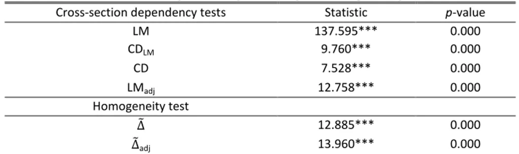
Countries to be dependent in terms of military spending is an expected situation. Therefore, implementing the tests, which allows the cross-section dependence and are accepted as the second generation panel data tests, in studies where the relationship between military spending and economic growth gives more reliable results. The cross-section dependence and slope homogeneity test results are seen in Table 1.
Table 1. Cross-Section dependency and slope homogeneity tests
Cross-section dependency tests Statistic p-value
LM 137.595*** 0.000
CDLM 9.760*** 0.000
CD 7.528*** 0.000
LMadj 12.758*** 0.000
Homogeneity test
12.885*** 0.000
adj 13.960*** 0.000
Note: *, ** and *** indicate statistical significance at 10, 5 and 1 percent level respectively
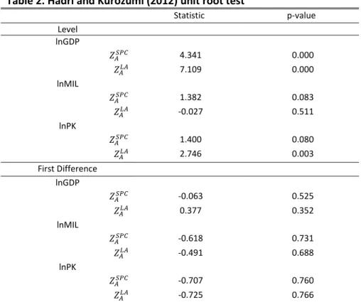
According to Pesaran and Yamagata (2008) test results, it is seen that the null hypothesis that represents the slope homogeneity assumption is rejected and the country-specific heterogeneity assumption is valid. It is supported the unit root, cointegration, cointegration estimator and causality tests to be implemented based on these findings should be second generation panel data tests. Hadri and Kurozumi (2012) panel unit root test results are seen in Table 2.
Table 2. Hadri and Kurozumi (2012) unit root test
Statistic p-value
Level lnGDP
4.341 0.000
7.109 0.000
lnMIL
1.382 0.083
-0.027 0.511
lnPK
1.400 0.080
2.746 0.003
First Difference lnGDP
-0.063 0.525
0.377 0.352
lnMIL
-0.618 0.731
-0.491 0.688
lnPK
-0.707 0.760
-0.725 0.766
Note: The maximum lag lengths were set to 3 and Schwarz Bayesian Criterion was used to determine the optimal lag length.
When the level values of the series are analyzed, it is seen that the null hypothesis that represents the stationary process for GDP and PK variables is rejected and is not rejected only for the MIL variable according to statistics. When the difference values of the series are analyzed, it is seen that the null hypothesis can not be rejected for all variables and the series become stationary.
is no cross-sectional dependence. In cases where the cross-sectional dependence is valid, it is seen that the cointegration relationship is valid between the series according to the bootstrap critical values.
Table 3. Westerlund and Edgerton (2007) cointegration test
Statistic Asymptotic p-value Bootstrap p-value LM bootstrap
4.554 0.000 0.149
Note: Bootstrap based on 10000 replications
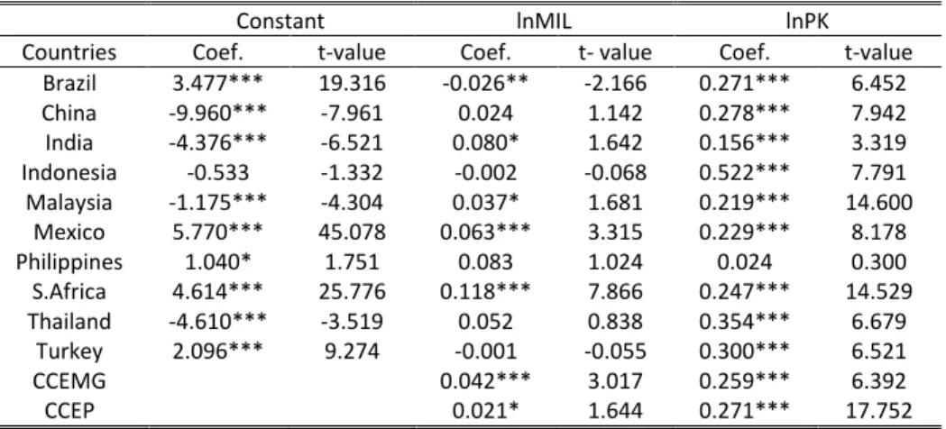
After the determination of the cointegration relationship between the series, the CCE estimator method is used to determine the coefficients separately for each country. When the results are analyzed, it is seen that the effects of military spending on economic growth are positive and significant in India, Malaysia, Mexico and South Africa. And in Brazil, it is seen that the effects of military spending on economic growth were negative and statistically significant. It is seen that there is not any relationship between military spending and economic growth in China, Indonesia, Philippines, Thailand and Turkey. The effects of real capital stock on economic growth are positive in all countries except for Philippines and statistically significant at the level of 1 percent. According to the results of common correlated effects mean estimator (CCEMG) and common correlated effects pooled estimator, it is seen that both military spending and real capital stock has positive effects on economic growth.
Table 4. Individual country CCE estimates for newly industrialized countries
Constant lnMIL lnPK
Countries Coef. t-value Coef. t- value Coef. t-value
Brazil 3.477*** 19.316 -0.026** -2.166 0.271*** 6.452
China -9.960*** -7.961 0.024 1.142 0.278*** 7.942
India -4.376*** -6.521 0.080* 1.642 0.156*** 3.319
Indonesia -0.533 -1.332 -0.002 -0.068 0.522*** 7.791
Malaysia -1.175*** -4.304 0.037* 1.681 0.219*** 14.600 Mexico 5.770*** 45.078 0.063*** 3.315 0.229*** 8.178
Philippines 1.040* 1.751 0.083 1.024 0.024 0.300
S.Africa 4.614*** 25.776 0.118*** 7.866 0.247*** 14.529 Thailand -4.610*** -3.519 0.052 0.838 0.354*** 6.679
Turkey 2.096*** 9.274 -0.001 -0.055 0.300*** 6.521
CCEMG 0.042*** 3.017 0.259*** 6.392
CCEP 0.021* 1.644 0.271*** 17.752
Note: *, ** and *** indicate statistical significance at 10, 5 and 1 percent level respectively
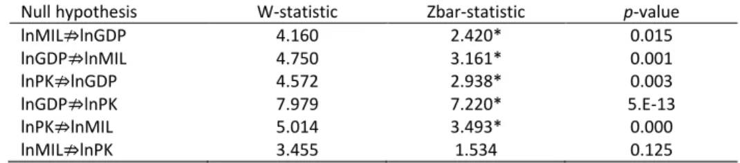
Table 5. Dumitrescu and Hurlin (2012) causality test
Null hypothesis W-statistic Zbar-statistic p-value
lnMIL lnGDP 4.160 2.420* 0.015
lnGDP lnMIL 4.750 3.161* 0.001
lnPK lnGDP 4.572 2.938* 0.003
lnGDP lnPK 7.979 7.220* 5.E-13
lnPK lnMIL 5.014 3.493* 0.000
lnMIL lnPK 3.455 1.534 0.125
Note: * indicates statistical significance at 1 percent level respectively. The results do not change with 1, 2, 3 lag structures.
In addition, while there is a causality relationship from real capital stock to real military spending, it is not determined any causality relationship from real military spending to real capital stock. According to Dumitrescu and Hurlin (2012) causality test, the feedback hypothesis is valid in the newly industrialized countries. When compared to previous studies, the result obtained in this study seems to support the studies of Chowdhury (1991), LaCivita (1991), Pradhan (2010) and Chang et al. (2015).
5. Conclusions and policy implications
In this study, the relationships between military spending and economic growth in Brazil, China, India, Indonesia, Malaysia, Mexico, Philippines, South Africa, Thailand and Turkey between the years 1988-2013 are analyzed through current panel data methods. Firstly, a strong degree of cross-sectional dependence and homogeneity are observed among the countries in the panel. This shows that a shock in one of the countries taking part in the panel affected the other countries as well, and each country has its own military policies. Then the second generation panel unit root test that is benefitted in case of cross-sectional dependence is valid is used and it is accepted that the level values of the surfaces are not stationary. For analyzing the long term relationship between the series, again it is made use of the cointegration estimator and the cointegration test that allows the cross-sectional dependence. And finally, the causal relationship between the series is examined.
and real military spending. The unidirectional causality exists from real capital stock to military spending.
Even if the feedback hypothesis is valid, policy recommendations to be made separately for each country would be more accurate in the newly industrialized countries group. Therefore, it is considered that reducing the military spending in India, Mexico and South Africa will lead to negative effects on economic activities and military spending should not be reduced. Reducing military spending and allocating the resources to more productive fields will be a rational policy for Brazil. Finally, reducing military spending will not create any effect on the economic activities of China, Indonesia, Philippines, Thailand and Turkey.
References
Atesoglu, H.S. (2002). Defense spending promotes aggregate output in the United States – Evidence from cointegration analysis. Defence and Peace Economics, 13(1), 55–60. http://dx.doi.org/10.1080/10242690210963
Aye, G.C., Balcilar, M., Dunne, J.P.,Gupta & R., Eyden, R.V. (2014). Military expenditure, economic growth and structural instability: a case study of South Africa. Defence and Peace Economics, 25(6), 619-633. http://dx.doi.org/10.1080/10242694.2014.886432
Barro, R.J. (1990). Government spending in a simple model of endogenous growth. Journal of Political Economy, 98(5), 103-125. http://dx.doi.org/10.1086/261726
Batchelor, P., Dunne, P. & Saal, D. (2000). Military spending and economic growth in South
Africa. Defence and Peace Economics, 11(6), 553–571.
http://dx.doi.org/10.1080/10430710008404966
Benoit, E. (1973). Defense and economic growth in developing countries. Boston: D.C. Heath & Company.
Benoit, E. (1978). Growth and defense spending in developing countries. Economic Development and Cultural Change, 34, 176-196.
Biswas, R. & Ram, R. (1986). Military expenditure and economic growth in LDC: An augmented model and further evidence. Economic Development and Cultural Change, 34(2), 361–372. http://dx.doi.org/10.1086/451533
Breusch, T. & Pagan, A. (1980). The LM test and its application to model specification in econometrics. Review of Economic Studies, 47(1), 239–253. http://dx.doi.org/10.2307/2297111
Cappelen, A., Gleditsch, N.P. & Bjerkholt, O. (1984). Military spending and economic growth in the OECD countries. Journal of Peace Research, 21(4), 361–373. http://dx.doi.org/10.1177/002234338402100404
Chang, T., Lee, C. C., Hung, K & Lee, K, H. (2014). Does military spending really matter for economic growth in China and G7 countries: The roles of dependency and heterogeneity.
Chowdhury, A.R. (1991). A causal analysis of defence spending and economic growth.
Journal of Conflict Resolution, 35(1), 80–97.
http://dx.doi.org/10.1177/0022002791035001005
Cuaresma, J.C. & Reitschuler, G. (2003). A nonlinear defence-growth nexus? Evidence from the US economy. Defence and Peace Economics, 15(1), 71–82. http://dx.doi.org/10.1080/1024269042000164504
Deger, S. & Smith, R. (1983). Military expenditure and growth in less developed countries.
Journal of Conflict Resolution, 28(2), 335–353.
http://dx.doi.org/10.1177/0022002783027002006
Deger, S. (1986). Economic development and defense expenditure. Economic Development and Cultural Change, 35(1), 179-196. http://dx.doi.org/10.1086/451577
Dumitrescu, E.I., & Hurlin, C. (2012). Testing for Granger non-causality in heterogeneous
panels. Economic Modelling, 29(4),1450-1460.
http://dx.doi.org/10.1016/j.econmod.2012.02.014
Dunne, P. & Vougas, D. (1999). Military spending and economic growth in South Africa.
Journal of Conflict Resolution, 43(4), 521–537.
http://dx.doi.org/10.1177/0022002799043004006
Dunne, P., Nikolaidou, E. & Vougas, D. (2001). Defence spending and economic growth: a causal analysis for Greece and Turkey. Defence and Peace Economics, 12(1), 5–26. http://dx.doi.org/10.1080/10430710108404974
Feridun, M., Sawhney, B. & Shahbaz, M. (2011). The impact of military spending on economic growth: The case of north Cyprus. Defence and Peace Economics, 22(5), 555–562. http://dx.doi.org/10.1080/10242694.2011.562370
Hadri, K., & Kurozumi, E. (2012). A simple panel stationarity tests in the presence of
cross-sectional dependence. Economics Letters, 115(1), 31–34.
http://dx.doi.org/10.1016/j.econlet.2011.11.036
Karagol, E. & Palaz, S. (2004). Does defence expenditure deter economic growth in Turkey? A cointegration analysis. Defence and Peace Economics, 15(3), 289–298. http://dx.doi.org/10.1080/10242690320001608908
Karagol, E. (2006). The relationship between external debt, defence expenditures and GNP revisited: the case of Turkey. Defence and Peace Economics, 17, 47-57. http://dx.doi.org/10.1080/10242690500369199
Kollias, C., Naxakis, C., & Zaranga, L. (2004). Defence spending and growth in Cyprus: a causal
analysis. Defence and Peace Economics, 15, 299-207.
http://dx.doi.org/10.1080/1024269032000166864
Kollias, C., Manolas, G. & Paleologou, S.Z. (2004). Defence expenditure and economic growth in the European Union: A causality analysis. Journal of Policy Modeling, 26(5), 553–569. http://dx.doi.org/10.1016/j.jpolmod.2004.03.013
Kollias, C., Mylonidis, N. & Paleologou, S. (2007). A panel data analysis of the nexus between defence spending and growth in the European Union. Defence and Peace Economics, 18(1), 75–85. http://dx.doi.org/10.1080/10242690600722636
Lai, C.N., Huang, B.N. & Yang, C.W. (2005). Defense spending and economic growth across the Taiwan Straits: A threshold regression model. Defence and Peace Economics, 16, 45–57. http://dx.doi.org/10.1080/1024269052000323542
LaCivita, C.J. & Frederiksen, P.C. (1991). Defense spending and economic growth, an alternative approach to the causality issue. Journal of Development Economics, 35(1), 117– 126. http://dx.doi.org/10.1016/0304-3878(91)90069-8
Lee, C.C. & Chen, S.T. (2007). Do defence expenditures spur GDP: A panel analysis from OECD and non-OECD countries. Defence and Peace Economics, 18(3), 265–280. http://dx.doi.org/10.1080/10242690500452706
McCoskey, S., & Kao, C. (1998). A residual-based test of the null of cointegration in panel data. Econometric Reviews, 17(1), 57–84. http://dx.doi.org/10.1080/07474939808800403 Pesaran, M.H. (2004). General diagnostic tests for cross section dependence in panels. (Cambridge Working Papers in Economics No. 0435), Faculty of Economics, University of Cambridge.
Pesaran, M.H., (2006). Estimation and inference in large heterogenous panels with multifactor error structure. Econometrica,Journal of the Econometric Society, 74, 967–1012. http://dx.doi.org/10.1111/j.1468-0262.2006.00692.x
Pesaran, M.H., Ullah, A. & Yamagata, T. (2008). A bias-adjusted LM test of error cross-section independence. Econometrics Journal, 11(1), 105–127. http://dx.doi.org/10.1111/j.1368-423X.2007.00227.x
Pesaran, M.H. & Yamagata, T. (2008). Testing slope homogeneity in large panels. Journal of Econometrics, 142(1), 50–93. http://dx.doi.org/10.1016/j.jeconom.2007.05.010
Pradhan, R. (2010). Modelling the nexus between defense spending and economic growth in Asean-5: Evidence from cointegrated panel analysis. African Journal of Political Science and International Relations, 4(8), 297–307.
Smith, R.(1980). Military expenditure and investment in OECD countries 1954–73. Journal of Comparative Economics, 4, 19–32. http://dx.doi.org/10.1016/0147-5967(80)90050-5
Swamy, P.A.V.B. (1970). Efficient inference in a random coefficient regression model.
Econometrica, 38(2), 311–323. http://dx.doi.org/10.2307/1913012
Westerlund, J., & Edgerton, D. (2007). A panel bootstrap cointegration test. Economics Letters, 97, 185–190. http://dx.doi.org/10.1016/j.econlet.2007.03.003