A bidimensional model of matching in the marriage market with women labor decision

FUNDAC

¸ ˜

AO GETULIO VARGAS

ESCOLA DE P ´

OS-GRADUAC

¸ ˜

AO EM ECONOMIA

Luiza Gueller Zardin

A Bidimensional Model of Matching in the Marriage

Market with Women Labor Decision

Luiza Gueller Zardin

A Bidimensional Model of Matching in the Marriage

Market with Women Labor Decision

Dissertac¸˜ao submetida a Escola de P´os-Graduac¸˜ao em Economia como requisito parcial para a obtenc¸˜ao do grau de Mestre em Economia.

Orientador: Carlos Eugˆenio da Costa

Ficha catalográfica elaborada pela Biblioteca Mario Henrique Simonsen/FGV

Zardin, luiza Gueller

A bidimensional model of matching in the marriage market with women labor decision /luiza Gueller Zardin. - 2016.

42 f.

Dissertação (mestrado)- Fundação Getulio Vargas, Escola de Pós-Graduação em Economia.

Orientador: Carlos Eugênio da Costa. Inclui bibliografia.

1. Economia - Modelos matemáticos. 2. Teoria dos casamentos. 3. Mercado de trabalho. 4. Mulheres - Emprego. I. Costa, Carlos Eugênio da. li. Fundação Getulio Vargas. Escola de Pós-Graduação em Economia. III. Título.

- - - ＭｾＭＭＭＭＭＭＭＭＭＭＭＭＭＭＭＭＭＭＭ

,..,.FGV

LUIZA GUELLER ZARDIN

A BIDIMENSIONAL MODEl OF MATCHING IN THE MARRIAGE MARKET WITH WOMEN LABOR DECISION.

Dissertação apresentada ao Curso de Mestrado em Economia da Escola de Pós-Graduação em Economia para obtenção do grau de Mestre em Economia.

Data da defesa: 22/03/2016

ASSINATURA DOS MEMBROS DA BANCA EXAMINADORA

ＦｕＢＧｅｾｴｯｳ｡＠ da Costa

Orientador (a)

/

￪ＬｾＢＢｊＢＮ＠

U:.ru'l.

_clJunw

Abstract

We construct a frictionless matching model of the marriage market where women have bidimensional attributes, one continuous (income) and the other dichoto-mous (home ability). Equilibrium in the marriage market determines intrahouse-hold allocation of resources and female labor participation. Our model is able to predict partial non-assortative matching, with rich men marrying women with low income but high home ability. We then perform numerical exercises to eval-uate the impacts of income taxes in individual welfare and find that there is con-siderable divergence in the female labor participation response to taxes between the short run and the long run.

Contents

1 Introduction 8

2 Literature Review 9

3 The Model 13

4 Equilibrium 19

a Existence . . . 19 b Characterization . . . 19 c A Particular Specification . . . 22

5 Taxation and equilibrium outcomes 26

6 Conclusion 30

Appendices 31

List of Figures

1

Introduction

An increasing concern in economics and policy making is inequality. Neverthe-less, the unitary approach often adopted in economic models treats the household as if consisting of a single decision maker, despite being indisputable that marriage plays an important role in the generation of welfare and its distribution both within and across households.

Furthermore, it is difficult to disentangle the interaction of the labor and the mar-riage markets, specially because whom one marries might determine how time is al-located in different tasks within the couple and also because the ability to perform certain tasks might lead to different choices of spouse.

This paper explores labor decisions and policy implications when female labor market participation and individual welfare are equilibrium outcomes of the mar-riage market. We build on a two-sided matching model of the marmar-riage market as in Becker (1973), where agents in the same household have transferable utility (TU).

Here couples make a decisions in the labor and marriage markets concomitantly and based on multidimensional traits. More specifically, we consider bidimensional attributes and allow women to allocate time in two different activities based on their bidimensional types and on whom they marry with.

Our hypotheses allow the simple characterization of the possible equilibria and a distinctive matching configuration arises in equilibrium. We are able to predict partial non-assortative matching: the men with the highest income renouncing the women in the top of the income distribution and marrying poorer high-ability women. However, if we consider only the households where the women join the labor market, matching is assortative.

The model also serves well our specific purpose of demonstrating some of the potential welfare implications of taxation in a multidimensional context with labor decisions. For a particular specification we perform numerical exercises and are able to illustrate impacts of policies for the welfare at the individual level. We find that the introduction of taxes benefits the housewives the most, mostly by a shift in the welfare division in such couples, with utility flowing from the husband to the wife.

female labor participation in the short and the long run, indicating that the interac-tion of the marriage and labor markets might play an important role in the effect of policies in the long run.

The outline of the rest of the paper is as follows. Section 2 reviews related litera-ture and Section 3 describes the model. Section 4 characterize the possible matching equilibria and specializes the model to the setting which we adopt in the numerical exercises of Section 5. Finally, Section 6 concludes.

2

Literature Review

In the last couple of decades the literature has taken important steps in the di-rection of addressing questions such as who marries whom and how couples make decisions, and two main strategies have been developed to attack these problems.

The collective approach of Chiappori (1988) and Apps and Rees (1988) makes solely one assumption: within each marriage Pareto efficient allocations are attained. Frequently, however, this model is further specialized in order to consider a Nash bargain game. The relative bargain power of each person can be represented either by his or her Pareto weight or by the assumed threat points. These are allowed to vary with prices, total income, and distribution factors, the latter being any variable that does not change the budget constraint or preferences but affect the weights. This framework provides insights into how the resources are allocated in a particular household by assuming that the Pareto weights are exogenously-given functions.

Alternatively, since Becker (1973) matching models have been employed in order to characterize the intra-household allocation of resources as an equilibrium out-come of the marriage market. As a result, it is possible to endogenously determine who marries whom, the division of marital output in every marriage, and the vari-ables that are able to shift the allocation of power between spouses. Since one of the goals of this work is to understand what are the policies that can change the al-location of marital output (and how they change it), it seems more appropriate to address this question with the use of matching models and this is the direction we follow here.

(TU) and agents on each side of the market characterized by a set of characteristics on which the matching takes place. Agents on one side of the market choose whom to match with on the other side of the market in order to maximize their own indi-vidual payoff. Due to the assumption of transferable utility, it is possible to condense the relevant information of a potential marriage into a surplus function, which is de-fined as the total utility generated in the marriage minus the sum of the utilities of each spouse when single.

Matching models in which individual traits are unidimensional have been largely studied, with the well-known result of positive assortative matching when the sur-plus function is supermodular, that is, the partners’ traits complement each other in the production of marital surplus.1 _{For instance, Chiappori and Oreffice (2008)} study the impact of innovations in birth control technology on intrahousehold al-location of resources by allowing men and women to differ in their preferences for children. Another interesting application of the unidimensional model is Chiappori et al. (2015), where an equilibrium lifecycle model of education, marriage and la-bor supply and consumption is considered and individuals match based on human capital.

Nonetheless, observed marriage patterns are much more complex and it is natu-ral to assume that there are sevenatu-ral traits one takes into account when contemplat-ing potential spouses. To brcontemplat-ing the restrictive outcomes derived by the nonfrictional unidimensional matching model more close to reality, there are two options. First, as was first done in Shimer and Smith (2000), it is possible to introduce frictions in the meeting process, which is then assumed to be sequential and random. Since agents discount their time, this implies that one does not wait for his or her perfect assorta-tive mate anymore and also that who marries whom has now a random component, features that resemble more those of the real world. The alternative to this is to keep a frictionless setting and allow multidimensionality.

Multidimensional settings, however, are difficult to theoretically characterize. In order to simplify the problem, some papers have attempted to condense several traits into a one-dimensional index. This approach was used in Chiappori et al. (2012) and allowed the authors to recover the marginal rates of substitution between

1_{More precisely, a functionf : R}2 _→ R_{is supermodular if, for every(x, y)and(x}′_{, y}′_{)such that}

characteristics such as body mass index and wages or education. However, this strat-egy might not represent well how multidimensional traits affect marriage decisions, a point that is emphasized in Dupuy and Galichon (2012). By rejecting the hypothe-sis that sorting occurs on a single dimension they show that individuals face impor-tant trade offs between the attributes of their spouses which are not amenable to a one-dimensional index combining the various characteristics.

Fortunately, beginning with Choo and Siow (2006), a large body of the literature2 has assumed that each individual can be characterized by a set of observable at-tributes and also by an unobserved heterogeneity, defined by characteristics that the researcher cannot observe but are relevant to the matching process.

This new branch of the literature builds on discrete choice theory and is therefore restricted to the case of discrete characteristics. Under some assumptions about the distribution of the unobserved heterogeneity, if there is a relatively small number of observable attributes, and if marital output is restricted to be independent of the interaction of the unobservables, it is possible to estimate the surplus generated by each couple and its division for an observed matching.

Testability would then come from the observation of several isolated marriage markets with the same surplus function but with different population characteris-tics. In practice, however, it is difficult to verify whether the considered markets in-deed have the same surplus function.

Also, this approach is clearly a powerful tool from an empirical perspective, but since multidimensional models have not been greatly explored in order to generate clear predictions from the theory, it is hard to disentangle the empirical results and understand their meaning.

Another point of concern is that currently there is no approach to handle sorting on multiple attributes if one of them is continuous, or, even if all of them are discrete, it might be the case that some of the unobservable traits interact with each other in the composition of the marital surplus, breaking a crucial hypothesis in Choo and Siow (2006). The present work sheds some light on both problems.

In this work we deviate from the current mainstream literature (e.g., Choo and Siow (2006)) and take a more theoretical approach as we look at a model for which

the primitives are the preferences and the household production function. We con-sider bidimensional attributes and the structure of the marriage market is very simi-lar to that of Quintana-Domeque et al. (2014). In their work, traits are also bidimen-sional: one continuous, representing socioeconomic status and the other dichoto-mous, indicating whether the individual is a smoker or not. Their starting point is a surplus function, which is supermodular in the socioeconomic traits of the couple and is affected by the spouses’ smoking status in a multiplicative way so that if at least one of the members of the household is a smoker, the surplus is diminished by a constant factor.

An important departure from their work is our formulation of how one’s own at-tributes interact in the generation of marital surplus. Since we further restrict the model so that a woman’s decision to allocate time in one type of occupation pre-cludes the participation in the other type and each activity requires a specific trait – income if the choice is for the labor market and home productivity for the alternative of home production – a person who is endowed with high levels of both attributes will not be able to apply them at the same time, eliminating any complementarity of traits.

In this aspect, our model resembles a sector model as in Roy (1951), whereas in Quintana-Domeque et al. (2014) there is the possibility of complementarity between a person’s own characteristics. For example, in their paper a nonsmoking man in a marriage with a nonsmoking woman generates strictly higher surplus than what would be generated in the marriage of a smoking man with the same socioeconomic status and the same woman. This leads to significant different matching patterns as the ones found in this paper, which are in turn similar to the patterns found in Low (2015), where matching is based in income and women’s “reproductive capital”. A major difference between the two papers is that in her work there are no labor deci-sions but there is a prior stage in which women decide whether to invest in human capital facing a trade-off between higher income and reduced fertility.

they develop a multidimensional matching model of the marriage market together with labor decisions in order to study the impact of taxes. Still, their work is based on Choo and Siow (2006) and is, therefore, empirical, facing limitations which will be discussed in the literature review section.

3

The Model

This section introduces a relatively general specification of the model, for which we are able to prove equilibrium existence and characterize it. Later, we specialize some of the described functions (utilities and distributions) in order to achieve fur-ther characterization and provide numerical examples.

This paper builds on a two-sided assignment model. We assume that individuals are characterized by their potential labor incomes, denotedx∈X = [

¯x,x¯]for women

andy ∈ Y = [

¯y,y¯]for men. Additionally, women can differ in an extra discrete

di-mensionα∈ { ¯

α,α¯}, which we denote home ability. Based on these traits, a matching game takes place, in which agents on one side of the market choose whom to match with on the other side in order to maximize their own individual payoff.

Transferable utility is commonly assumed in the literature of family economics since it implies a one-to-one utility exchange rate within the household which al-lows us to summarize the marital output from any match in a single number. This greatly simplifies equilibrium characterization. Here, we condense all the relevant information of a potential marriage into the total utility function.

With the purpose of improving tractability, we consider that couples make labor decisions in a very simplistic way. Since women have both home ability and income characteristics, they face a trade-off between boosting home production or joining the labor force and increasing the household total income. We allow them to de-cide where to allocate their time, but the choice of one activity precludes the other, leaving them with the binary decision of whether to work (t=1) or not (t=0).

The total utility generated within any particular household can be decomposed in two parts that interact in a multiplicative way:

U(x, α, y, t) =f(t

¯

In the first part, the increasing function f : R_{+ →} R_{++ accounts for how the}

female home ability dimension might increase (or not) the total household utility. The second term,g :R_+→R_{+, depends on the total earned income of the household}

and is assumed to be three times differentiable. We further request thatg(0) = 0, g′

>

0, g′′_>0

andg′′′ _≤0

.

The assumption thatg′′

> 0implies that the total household utility is supermod-ular in the spouses’ income. Moreover, g′′′

< 0 implies that the surplus function is not ”more” supermodular the higher the couple’s total income. For example, if we consider three women (x,x+δ andx+ 2δ) and three men (y,y+σand y+ 2σ), the gains from the assortative matching (versus nonassortative matching) of the pair (x,x+δ) with the pair (y,y+σ) are higher than the gains that arise from the assor-tative matching (versus nonassorassor-tative matching) of the pair (x+δ,x+ 2δ) with the pair (y+σ,y+ 2σ).3 _{We need this hypothesis for later proof of the equilibrium} char-acteristics, more specifically to show that once a many∗

marries a woman who stays at home in equilibrium, every men with higher income also does so.

In order to account for the possibility of singles, we introduce fictional types in each side of the market. If a woman is single, we represent her partner as man ∅_y

and assume their union generates no surplus relatively to the woman being sin-gle. Clearly a single woman will always join the workforce since otherwise her utility would be the lowest possible. Analogously, if a man is single, we represent his wife as

∅_{xand in the same way assume there is no surplus from their fictional marriage.}

To simplify the notation, we introduce the superscripts S, W and H to denote whether the function refers to a household composed, respectively, of a single per-son, a couple in which the woman works or a couple in which the woman contributes to home production.

Giving the so far exposed, singles’ utility only depends on labor income (z ∈X∪Y) and can be written as

US_{(z) =f(}

¯

α)g(z).

3_{g(x+y) +g(x+δ+y+σ)−g(x+δ+y)−g(x+y+σ)> g(x+δ+y+δ) +g(x+ 2δ+y+ 2σ)−}

Differently, a couple’s total utility will depend on labor decisions according to

UH(x, y, α) =f(α)g(y)

UW(x, y, α) =f(

¯

α)g(x+y),

which results in a total utility of

U(x, y, α) = max{UH(x, y, α), UW(x, y, α)}.

The hypotheses made so far imply that there are no gains from the interactions between the ability dimension of spouses (since men here have no ability) and be-tween the ability and wage dimensions of the same individual (since women cannot split their time between activities). What persists is a potential synergy between the spouses’ wages if both of them work and between the wage of one of them and the ability of the other otherwise. This allows the simple characterization of the possible equilibria, which are not totally assortative in income, and also serves well our spe-cific purpose of demonstrating some of the potential welfare implications of taxation in a multidimensional context with labor decisions.

It is customary in the TU matching literature to represent a match by the total surplus it generates, instead of the total utility as we have done so far. In accordance, we can write the surplus for each case as

SH_{(x, y, α) =U}H_{(x, y, α)−U}S_(x)−US_(y)

SW(x, y, α) =UW(x, y, α)−US(x)−US(y)

which results in a final surplus of

S(x, y, α) = max{SH(x, y, α), SW(x, y, α)}.

it is equivalent to formulate the matching problem in terms of any of these functions. Because some of the utilities presented so far depend only on a subset of the types, we will simplify the notation and omit the irrelevant variables whenever it is convenient.

Given these functions, women and men take part in a one-to-one matching game where a woman’s type is characterized by (x,α) ∈ X˜ = X × {

¯

α,α¯} ∪ {∅_{x} and a}

man’s type is solely his income y ∈ Y˜ = Y ∪ {∅_{y}. The income measures of low}

ability women, high ability women and men are respectively denoted

¯γx : X →

R_+,

¯

γx : X → R+, andγy : Y → R+ and are assumed to be absolutely continuous with

respect to the Lebesgue measures on each set.4

In this context, a matching is a measureγon the product spaceX˜ ×Y˜, the pro-jections of which coincide with the initial distributions on each set.

A matching is said to be pure if almost all agents are matched with probability 1 to exactly one other agent, that is, ifγ takes values in{0,1}almost everywhere in

˜

X×Y˜. If this is the case, then there is a bijection betweenX˜ andY˜ which defines for any woman (any man) who she (he) is married to. As we shall later see, this does not need to be the case in the equilibrium defined below.

The stable matching concept of Shapley and Shubik (1971) is the relevant equi-librium definition in this framework. A matching is said to be stable if (i) there is no man and woman who would both prefer to be married to each other rather than re-main in their current situation, and (ii) there is no married person who would rather be single.

The mass of the types∅_xand∅_{y will be an equilibrium outcome. Since any}

mar-riage in which both spouses have strictly positive labor incomes generates a strictly positive surplus, the definition of stable matching implies that in equilibrium there will only be singles if there is an excess mass of people in one of the sides of the market, in which case the side in excess supply will have singles. It is without loss of generality to assume that the male population has measureγy(Y) = 1and that

the total mass of women is

¯

γx(X) + ¯γx(X) = µ > 1, since this would not change the

equilibrium matching patterns except for which side of the market bares the singles. Therefore, there will be a total ofµ−1men of type∅_{y and no woman of type}∅_{x in}

4_{The associated probability distributions are denoted}

¯

equilibrium.

Additionally, we definep= γ¯x(X)

µ as the fraction of high ability women in the total

population and assume thatpµ <1and(1−p)µ <1, so that at least some women of both ability types are married.

Underlying any particular stable matching, there are payoff functions that sup-port it as an equilibrium outcome. We denote these functionsu(x, α)for women and

v(y)for men. Since the utilityUW _{generated in a marriage in which the woman works}

does not depend on the woman’s home ability, it follows from the definition of a sta-ble matching that if(x,

¯

α) and(x,α¯) work with positive probability in equilibrium, thenu(x,

¯

α) = u(x,α¯) ≡ uW_{(x), since no woman would accept to be in a marriage if}

she can get a higher payoff in another. Analogously, if two women(x′

,α¯)and(x′′

,α¯)

stay at home in equilibrium with a positive probability, thenu(x′

,α¯) = u(x′′

,α¯), since no man married to a woman who stays at home would accept offering her more than the payoff that any other woman who stays at home gets.

Bearing this in mind, we simplify the notation as follows:5

u(x, α) =

(

uW(x) if the woman(x, α)works

uH if the woman(x,α¯)stays at home.

For what follows, we assume that at least some high ability women join the work-force.6 _{As a consequence, the payoffu}H _{of the women who stay at home is pinned}

down by the greater outside option that a woman who makes this decision has, that is

uH _{= sup} x∈XH

uW_(x),

whereXH _{⊆X is the subset of women who have a positive probability of being in a}

marriage in which they stay at home in equilibrium.

It is a direct consequence of the stable matching definition that the resulting

util-5_{Note that no woman with the low ability type will stay at home in equilibrium.}

6_{This will be the case if eitherα¯is not too high or if the maximum income in the support ofγ¯is}

itiesuW_{(x)of any woman who work and the utilitiesv(y)of any man satisfy}

uW(x) +v(y)≥UW(x, y)∀x∈X∀y∈Y (1)

uH +v(y)≥UH(y)∀y∈Y, (2)

since otherwise it would be possible for a man and a woman to marry and get payoffs strictly higher than what they would get in equilibrium. If woman(x, α)and many

are married and woman(x, α)works in equilibrium, then equation (1) holds if equal-ity. In the same way, if woman(x, α)and manyare married and woman(x, α)stays at home in equilibrium, then equation (2) holds with equality.

This in turn implies two separate maximization problems. One for women,

uW(x) = max

y∈Y U W

(x, y)−v(y) (3)

and the other for men

v(y) = max{max

x∈X U

W_{(x, y)−u}W_{(y), U}H_(y)−uH_{}. (4)}

If we consider only couples where the woman works in equilibrium, then match-ing becomes unidimensional and, becauseUW_{(x, y)is supermodular, the matching}

must be positively assortative in income (Becker (1973)). Therefore, spouses in mar-riages where the woman works are assigned to each other with probability one in equilibrium.7 _{This allows us to describe who marries whom in marriages where the} woman works by bijective functions. We let ψ(x) denote the husband of womanx

andφ(y)the wife of many. Obviously we have thatψ(φ(y)) = y.

Hence, the solution to problem (3) can be obtained by integration of the following envelope condition

∂uW_(x)

∂x =

∂UW_{(x, y)}

∂x |y=ψ(x).

Because the utility of single women is pinned down by equation (3), we can use it as an initial condition, yielding

7_{This need not be true for the cases where one of the spouses is indifferent between a marriage}

uW(x) =US(xS) +

Z x

xS

∂UW_{(x, ψ(x))}

∂x dx∀x > xS,

wherexSis the single woman with the highest income.

4

Equilibrium

a

Existence

The existence of a stable matching is guaranteed by a very general result that states the equivalence between a particular stable matching in a multidimensional transferable utility context and a particular solution to an optimal transportation problem. More precisely, a matching γ is stable if and only if it is also a solution to the maximization of aggregate surplus over all possible measures on the product space X˜ ×Y˜. Since the setX˜ ×Y˜ is a compact subset of a compact metric space, the set of measures on X˜ × Y˜ is also compact. Combining this with the fact that the surplus function is continuous, there is a solution to the above mentioned trans-portation problem. The payoffs that support a measure as a stable matching can be obtained from the solution of a dual problem.8

b

Characterization

Proposition 1(Characterization of the set of stable matchings). In any stable match-ing there exists cutoffsy∗

∈Y andxT, xS ∈Xsuch that:

(i) Women of type(x,

¯

α), withx < xS are single with probability one:

γ(B,

¯

α,∅_{y) =}

¯γx(B)∀B ∈ B(

R_)∩[

¯x, xS).

(ii) Women of type(x,α¯), withx < xT do not work with probability one:

γ(BH_{,α,¯ Y}˜_{) = ¯γ}

x(B)∀B ∈ B(R)∩[

¯

x, xT), whereBH ={x∈B|uH > u(x)}.

(iii) Women of type(x,α¯), withx > xT work with probability one:

γ(BW_{,α,¯ Y}˜_{) = ¯γ}

x(B)∀B ∈ B(R)∩(xT,x¯], whereBW ={x∈B|u(x)> uH}.

(iv) Men of type y, withy > y∗

marry women of type(x,α¯), withx≤xT with

proba-bility one:

γ(XH_{,α, B¯ ) = γ}

y(B)∀B ∈ B(R)∩[y∗,y¯], whereXH ={x∈X|x≤xT}.

(v) Men of type y, withy < y∗

match with women who work positive-assortatively in income:

γ(φW_{(B),α, B¯ ) +γ(φ(B),}

¯

α, B) =γy(B)∀B ∈ B(R)∩[

¯y, y

∗

), where

φW_{(B) ={x∈φ(B)|x > x}

T}.

Proof. In the Appendix.

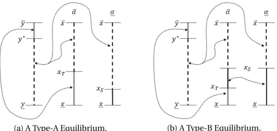
A direct way of grasping Proposition (1) is through Figure (1). The structure out-lined in the proposition gives rise to two classes of equilibria, depending on whether

xT > xS or otherwise. The first diagram in Figure (1) represents the Type-A

equilib-ria, wherexT > xS. In this case, the bijective functions that represent the matches

where the woman works can be determined from:

1−Fy(y∗) = ¯Fx(xT)

¯

Fx(xS) =µ−1

Fy(ψ(x)) =

¯

Fx(x)−

¯

Fx(xS)ifx∈(xS, xT]

Fy(ψ(x)) =

¯

Fx(x)−

¯

Fx(xS) + ¯Fx(x)−F¯x(xT)ifx > xT.

Analogously, the second diagram in Figure (1) represents the Type-B equilibria, wherexT ≤xS. In this case, the high ability womanx ∈ (xT, xS)are also single and

the corresponding matching functions are obtained from:

1−Fy(y∗) = ¯Fx(xT)

¯

Fx(xS) + ¯Fx(xS)−F¯x(xT) = µ−1

Fy(ψ(x)) =

¯

Fx(x)−

¯

Fx(xS) + ¯Fx(x)−F¯x(xS).

Everything else held constant, the higher the ratioα/¯ ¯

α, the largest the cutoffxT

(a) A Type-A Equilibrium. (b) A Type-B Equilibrium.

Figure 1: The two types of equilibrium. Same patterns in the two sides of the mar-ket indicate which group of men marry which group of women. For the dotted line group, matching is assortative in income and therefore unique. Couples of the dou-ble line group might be formed by any two individuals, one of each side, and the equilibrium definition even allows for randomization. Single women are indicated by the fainted line, and in the equilibria of Type-B they are of both low and high abil-ity.

It is noteworthy that in the Type-B Equilibrium the women of the high home abil-ity type who are single have higher income than the ones of the same abilabil-ity type who are married and stay at home. This has to be the case since if there were a single woman of high ability with incomex′

and another woman with high ability who mar-ries and stays at home with incomex′′

, such thatx′

< x′′

, then(x′′

,α¯)’s husband could offer(x′

,α¯)a payoffU for her to stay at home such thatu(x′′

,α¯) > U > u(x′

,α¯). In

this case both him and woman(x′

,α¯)would be better off, breaking the equilibrium. A feature that stands out is that the described equilibria need not be pure, since spouses in couples(x, α, y)wherex∈[0, xT], α= ¯αandy > y∗are actually indifferent

between any other partner in the same subspace of types. It follows that there are multiple equilibria. Yet, it might be the case that the cutoffsxT,xSandy∗are unique,

but so far we haven’t been able to proof this for a general surplus function.

c

A Particular Specification

Here we introduce the primitives of an economy where the total utilities of the households are a particular case of the model we have explored so far. This results in a quadraticg, which is also considered in Quintana-Domeque et al. (2014).

Agents derive utility from the consumption of a marketable private good and also from a public good which is produced within the household and exclusively con-sumed by its members.

Each person cares only about his or her own consumption of the two types of goods in the economy and individual utility takes the following form:9

Vi(qi, P) = qiP

whereqiis the private consumption of agentiandP is the household public good.

This utility is a particular case of the generalized quasi-linear (GQL) form of Bergstrom (1989) and accomplishes two goals.10 _{First, utility transfers between spouses can be} achieved by shifting the division of the private good and holding public good con-sumption fixed. Second, there is always a positive surplus from marriage due to the presence of the public good.

The public good can be produced using the private good and time at home t ∈ {0,1}according to the following production function:

P(Q, t, α) = [t

¯

α+ (1−t)α]Q

where,Qis the amount of private good used in the production and, as before,t = 0

if the woman contributes to home production andt = 1otherwise.

First we consider the decision faced by a single woman with wage dimensionx. If a single woman decides to contribute to the home production, she will have no earnings and, therefore, no consumption. As a result, irrespective of their ability di-mension, singles always join the workforce. Therefore, their problem can be written as

9_{The same utility is used in Chiappori et al. (2009) and Browning et al. (2014).} 10_{The GQL preferences are represented byu}

i(qi, P) =F(P)qi+Gi(P)and in the case of only one

max

q,Q ¯αqQ

subject toq+Q≤z

with resulting utility

US_{(z) =}

¯

αz2/4. (5)

Couples, on the other hand, have the possibility of specialization, so labor deci-sions are now part of the problem. As before, some women have high home ability and, therefore, are capable of increasing the home productivity from

¯

αtoα¯.

If either the woman’s ability is low or it is efficient for her to join the workforce, then any efficient allocation of resources within the couple where both spouses con-sume positive amounts must solve

max

qF,qM,Q¯

α(qF +qM)Q

subject toqM +qF +Q≤x+y

generating a total utility for the couple of

UW_{(x, y) =}

¯

α(x+y)2/4.

Otherwise, if the woman joins the workforce the household problem becomes

max

qF,qM,Q

¯

α(qF +qM)Q

subject toqM +qF +Q≤y,

in which case the total output is given by

UH_{(x, y) = ¯αy}2_/4.

We have previously assumed that the couples’ labor and consumption decisions were efficient and this indeed has to be the case in any stable equilibrium. This is true since otherwise a close substitute to one’s partner would be able to offer more utility in an efficient union and both would be better off together.

work-force. Also, because there is a public good, any marriage generates a positive surplus so that in equilibrium only a measure µ−1of women are single and every man is married.

Comparing this setting with our more general model, we can see that this is a specific case if we consider the function f as the identity and g(z) = z2_{/4. These}

functions satisfy all the restrictions we imposed before and therefore Proposition (1) applies here.

Since single women’s utilities are pinned down by equation (5), the whole util-ity profile of working women is related to uW_(x

S). If both sides had the same mass

of individuals (if we allowed µ = 1), then there would be no single person at the stable equilibrium. In this case, the division of marital output between men and women would be pinned down only up to a constant determined by how much sur-plus each side would get at the worst marriage. In turn, if we considered more men than women, there would be single men in equilibrium and thus the utility of the single man with the highest income would shape the utility profiles.

Finally, we consider uniform income distributions with support in [0,1]. A more complex distribution would play a role in determining the utilities in equilibrium, since the local scarcity of any gender is a well-known distribution factor, but would not change the more general equilibrium patterns.

Since income distributions are uniform, in any Type-A Matching xT and xS are

given by

xaS =

µ−1

µ(1−p) x

a

T =

1−y∗

µp . (6)

The indifferent man y∗ _{is determined by the equality in equation (A.1), together}

with the definitions in equation (6).

Therefore, we can determine the matching functionψ(x)that describes the hus-band of womanxas

ψa(x) =

(_{µ(1−p)(x−x}

S) if x∈[xS, xT] (7a)

Likewise,φ(y)describes the wife of manyas

φa(y) =



 

 

xS+

y

µ(1−p) if y∈[0, y0) (8a)

y

µ+pxT + (1−p)xS ify∈[y0, y

∗

]. (8b)

Therefore, the solution to problem (3) can be written as:

uW(φa(y)) =



 

 

uW(xaS) + ¯

α

4(1 +µ(1−p))[(y+φ

a

(y))2−(xaS)2] ∀y∈[0, y0) (9a)

uW_(xa

T) + ¯

α

4(1 +µ)[(y+φ

a_(y))2_−(y

0+xaT)

2_{] ∀y∈[y}

0, y∗]. (9b)

The same reasoning can be applied to Type-B equilibria, resulting in the following cutoffs:

xbS =

µ−y∗

µ x

b

T =

1−y∗

µp . (10)

Therefore, we can define the matching functionψ(x)that describesx’s husband if she works as

ψb_{(x) = µ(x−x}

S)if y∈[xS,1] (11)

Likewise,φ(y)describes they’s wife as

φ(y)b =xS+

y

µif y∈[0, y

∗

] (12)

Therefore, the solution to problem (3) can be written as:

uW_(φb_{(y)) =u}W_(xb

S) + ¯

α

4(1 +µ)[(y+φ

b_(y))2_−(xb

S)2] ∀y∈[0, y ∗

]. (13) In the appendix we provide a proof of Proposition (1) for this specific setting, which also guarantees the uniqueness of the cutoffs.

Proposition 2. If the surplus function is quadratic and the income distributions are uniform, the cutoffsxT,xS, andy∗are unique.

5

Taxation and equilibrium outcomes

An advantage of modeling labor and marriage decisions together is the possibility to evaluate the impact of policies in both markets. With the next proposition and the numerical exercise we intend to clarify some of the potential impacts of taxation in the equilibrium outcomes. Before all else, it is important to observe that the proof of Proposition (1) still holds if we introduce a linear income tax for individuals.

The following proposition illustrates how a policy supposedly intended to benefit married women might have the opposite consequence due to equilibrium adjust-ments.

Proposition 3. Consider a small proportional taxτon men’s income used to increase the potential income of every married woman byΓand suppose the original equilib-rium is of the Type-B Matching withy∗ _{∈ (0,1)}

. Then, the cutoffxT is reduced, and,

consequently, the proportion of married women in the labor market is increased. Also, every nonworking married woman is made worse off.

This simple result is a direct consequence of the fact that the utility of single women is not changed in the new equilibrium and that the crowding out of the home activity pushes downwards the utilities of all the women who stay at home.11 _Yet, this type of conclusion cannot be reached in a perfectly assortative unidimensional model.

Now, in a numerical exercise we intend to show how the utility profiles and the welfare division within and across couples change in response to linear taxation. With this example we are also able to expose major differences between the long and short run income elasticities of the marginal high ability woman. In the short run, we expect marriage market equilibrium to be sustained given any small change in the parameters of the model if we assume that there is a strictly positive cost from divorce. On the other hand, as time passes, new marriages are formed and, for rea-sons exogenous to the model, some marriages are broken, implying a long-run ten-dency towards a new equilibrium. We find that the long run elasticity is much higher than the short run.

11_{An increase in the potential income of every married women without changing the income}

For this, we assume that income is taxed at a linear rate t. In order to keep the government budget balance at a constant level, we assume that each individual re-ceives a lump-sum transferT, which is independent of his or her marital status and sex, and in such a manner that there is no tax revenue.

Also, we choose a specific parametrization such that there is 5% more women than men (µ=1.05), the high ability women have a home productivity three times that of the low ability (α¯

¯

α=3) and correspond to half of the female population (p=0.5).

Without any taxes, the equilibrium results in 43% of the high ability women stay-ing at home, which corresponds to 23% of all the marriages.

Next, we assume a welfare function of the form

W =R

x∈Xw(u(¯α, x))d¯γx(x) +

R

x∈Xw(u(_¯α, x))d

¯γx(x) +

R

y∈Y w(v(y))dγy(y),

wherew(z) =z0.5_.

Our taxation design problem is based on an individualistic social welfare func-tion, with inequality both within and across households adversely affecting social welfare. Note that it is necessary to introduce some curvature in the welfare func-tion because otherwise the supermodularity of the couples’ total utilities would im-ply a maximum income inequality in the optimal. With this specification, we obtain an optimal linear tax rate of t = 23.6% and a corresponding lump-sum transfer of

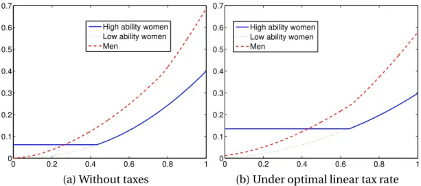
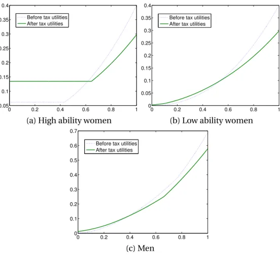
T = 0.1056. In this optimal setting total welfare is increased by 2% and we illustrate the variations that occur in the utility profiles of the individuals in Figures (2) and (3).

0 0.2 0.4 0.6 0.8 1

0 0.1 0.2 0.3 0.4 0.5 0.6 0.7

High ability women Low ability women Men

(a) Without taxes

0 0.2 0.4 0.6 0.8 1

0 0.1 0.2 0.3 0.4 0.5 0.6 0.7

High ability women Low ability women Men

(b) Under optimal linear tax rate

0 0.2 0.4 0.6 0.8 1 0.05

0.1 0.15 0.2 0.25 0.3 0.35 0.4

Before tax utilities After tax utilities

(a) High ability women

0 0.2 0.4 0.6 0.8 1

0 0.05 0.1 0.15 0.2 0.25 0.3 0.35 0.4

Before tax utilities After tax utilities

(b) Low ability women

0 0.2 0.4 0.6 0.8 1

0 0.1 0.2 0.3 0.4 0.5 0.6 0.7

Before tax utilities After tax utilities

(c) Men

Figure 3: Utility profiles for each discrete type.

Clearly, the introduction of taxes benefits the housewives the most. This is mostly due to the mechanical change in the equilibrium cutoffxT, since with higher taxes

more women will decide not to work and the equilibrium payoff of all such women is pinned down by the utility of womanuW_(x

T), which is increasing inxT.

The introduction of taxes raises the cutoffxT since it increases the comparative

advantage of higher home productivity. The new percentage of high ability women staying at home is 64%, which corresponds to 34% of all the marriages.

From here on, the subscripts 1 and 2 will represent the equilibrium variables in the short and long run, respectively.

In order to draw a parallel, we evaluate the impact of a 1% decrease in the tax rate starting from the optimal taxation (from t=23.6% to t=23.36%), which induces a change inxT fromxT,1 = 0.6449toxT,2 = 0.6426, pushing all women[xT,2, xT,1]into

the labor market and leading womanxT,2 to be indifferent between marrying man

yT,2in[y∗2,1]and staying at home or marrying manψ2(xT,2)and working. Hence, a 1%

in female labor market participation in the long run.

Now, if we fix the matchings to be as in the first equilibrium, what percentage change in the tax rate would be needed for the woman xT,2 to join the workforce?

In this case, we should compare the utility generated in the marriage between her and her husband yT,1 in [y∗1,1] in each situation. This means finding t such that

UW_(x

T,2, yT,1)|t+δ> UH(yT,1)|t+δ and UW(xT,2, yT,1)|t−δ< UH(yT,1)|t−δ for any δ > 0.

SinceyT,1might be any men in[y1∗,1], there is actually an interval of possible tax rates.

IfxT,2 is married toy1∗, the indifference tax rate would be t=19.46%, whereas ifxT,2 is

married toy = 1, there is no positive tax rate that would make the couple better of if

xT,2decided to work.

Consequently, we see that in the short run, the minimum percentage decrease in the tax rate starting from the optimal that would prompt woman xT,2 to work is

17.6% (from t=23.6% to t=19.46%), which is much higher than the 1% needed in the long run. Since similar results are obtained for different parameter specifications, these numbers illustrate the potential relevance of modeling the labor and marriage markets together, specially for a better understanding of the long run elasticities of labor supply.

In this example, the labor market participation elasticity in the short run would be zero, since small changes in wages would have no effect in female labor market par-ticipation because of the wedge between the husband womanxT has in equilibrium

if she works (ψ(xT) < y∗) and the man she marries if she stays at home (y ∈ [y∗,1]).

Still, the contrast of the 1% needed in the long run vs. the 17.6% needed in the short run can be interpreted as a comparison between some kind of inverse female labor participation elasticities.

possibly make participation decisions less sensitive to tax changes and perhaps the differences seen in the long and short run ”participation elasticities” would be less pronounced. Nevertheless, this example indicates an important and not explored mechanism affecting labor supply responses, at least in the long run.

6

Conclusion

In this paper we have presented an integrated model of the marriage market and female labor supply. The model main features are the bidimensional traits of women, our specification of how those traits are able to interact in the generation of marital surplus, and, of course, the inclusion of women labor decisions. These characteris-tics are relevant since multidimensional attributes have not been greatly explored in the literature and the papers that have ventured in this direction lack at least one of the other two cited features.

Our model is able to generate non-monotonic matching on income on the mar-riage market, since the men at the top of the income distribution forgo marrying their female counterparts in order to mate with high home ability women.

For a particular setting, where the surplus function is quadratic and the param-eters of the model are chosen, we illustrate the impacts of policies for the welfare at the individual level. We see that a great share of welfare gains is due to an incre-ment in the utility of housewifes, essentially because with higher taxes more women choose not to join the labor market and the equilibrium payoff of all housewifes is determined by the outside option of the one with the highest income.

Appendices

a

Proof of Proposition 1

First note that it must be the case that every high productivity woman who does not work in equilibrium gets the same payoff uH_{. Suppose this is not the case, so}

there exists two women(x1,α¯)and(x2,α¯)who do not work in equilibrium and such

thatu(x1,α¯)> u(x2,α¯). Their husbands are denoted respectivelyy1andy2, with

pay-offsv(y1)andv(y2). Then, sinceUW(x1, y1) = UW(x2, y2) = UW(x2, y1), it would be

possible for x2 to offer many1 payoffv(y1) +δ and get herself a payoffu(x1,α¯)−δ,

which is strictly higher thanu(x2,α¯)for someδ >0close enough to zero.

Second, suppose the woman (x,α¯)works, marries the manψ(x), and get payoff

uW_{(x)in equilibrium. Then, since any woman(x}′

,α¯)withx′

> xcan also marryψ(x),

work and get payoffUW_(x′

, ψ(x))−v(ψ(x))> UW_{(x, ψ(x))−v(ψ(x))> u}H_{, therefore}

in equilibrium(x′

,α¯)also works. In the same way, if the woman(x,α¯)marries and stays at home in the equilibrium, then any woman(x′

,α¯)withx′

< xalso stays at

home, sinceuH _{> U}W_{(x, y)−v(y)> U}W_(x′

, y)−v(y)∀y.

These reasoning implies that if there is an equilibrium, there must be a cutoffxT

such that every woman(x,α¯)withx > xT works and every woman(x,α¯)withx < xT

stays at home.

Now we consider men. For this, we define the following function

Z(x, y)≡UW(x, y)−uW(x)−UH(y) +uH.

We can write its derivative with respect toyas

Z′

(x, y)≡ ∂Z(x, y)

∂y =f(α¯)g

′

(x+y)−f(¯α)g′

(y)

and the second derivative is

Z′′

(x, y)≡ ∂

2_{Z(x, y)}

∂y2 =f(_¯α)g

′′

(x+y)−f(¯α)g′′

(y)<0

where the inequality follows from the assumption thatg′′′

(.)≤0andα >¯

¯

α.

Suppose by contradiction there existsy >ˆ

woman who does not work in equilibrium and, with abuse of notation, letyˆdenote the man with the highest income among those. Becauseµp < 1,y <ˆ y¯. Since man

ˆ

y+δmarries a woman who works in equilibrium, by the continuity of the equilibrium utilities, it must be thatyˆis indifferent between marrying a womanx′

who works or any woman who stays at home. Also, because the matching is assortative among the marriages where both spouses work and the income measures are absolutely contin-uous, it must be thatx′

=xS.

ThenZ(xS,yˆ) = 0andZ(xS,0) =f(

¯

α)g(xS) +uH −uW(xS).

IfxS < xT,Z(0) > 0. Else,uW(xS) = f(

¯

α)g(xS), andZ(0) > 0. SinceZ′′ < 0and

Z(xS,0) > Z(xS,yˆ), it must be thatZ′(xS,yˆ) < 0. But thenZ(xS,yˆ−δ) > 0forδ > 0

small enough, a contradiction. Therefore, there existsy′

such that every many≤y′

marries a woman who works in equilibrium. With abuse of notation, let y′

be the man with the highest income among them. Then either y′

= ¯y and all men marry women who work, or y′

< y¯

and y′

is indifferent between marrying a woman who stays at home and a woman

x′

= φ(y′

) who works, since for any δ > 0 small enough we have that UW_(φ(y′

−

δ), y′

−δ)−u(φ(y′

−δ),α¯)≥UH_(y′

−δ)−uH _andUW_(φ(y′

+δ), y′

+δ)−u(φ(y′

+δ),α¯)≤

UH_(y′

+δ)− uH _{and all functions are continuous. Suppose by contradiction that}

there is a man y′′

> y′

who marries a woman x′′

who works in equilibrium. Then, by the same argument as before, there must be a man y′′′

∈ (y′

, y′′

) such that he is also indifferent between marrying a woman x′′′

who works and another woman who stays at home, and such that every men in(y′

, y′′′

)prefer to marry women who stay at home. Note that it must be the case that x′

= x′′′

, since for couples where both spouses work marriage is positive assortative in the income dimension and the measures are absolutely continuous. This implies thatZ(x′

, y′

) =Z(x′

, y′′′

) = 0. Because we assumed that every manyiny∈ (y′

, y′′′

)marries a woman who stays at home in equilibrium, it must be thatZ′

(x′

, y′

)≤0, a contradiction withZ(x′

, y′′′

) = 0, sinceZ′′

<0.

Finally note that if we applied a transformation I, such that I′

> 0 andI′′

con-ditions involving up to the third derivative of I so that the proposition would also hold. In this case, more restrictions are necessary, since otherwise the progressivity of the tax schedule could also offset the supermodularity of the surplus function, and undermine the remaining assortativeness.

b

Proof of Proposition 2

We provide a constructive proof of the existence of the equilibrium for the specific case of quadratic surplus and uniform income distributions. In this particular case, we show that there is only one possible candidate fory∗

for each parameter vector, and that therefore the cutoffs are unique.

In order to prove that there exists a stable matching of the proposed form, it is sufficient to show that we can findy∗

∈[0,1]such that the following three equations hold:

v(y) =UH(y)−uH ≥UW(x, y)−uW(x)∀y≥y∗

∀x (A.1)

v(y) =UW_{(φ(y), y)−u}W_{(φ(y))> U}H_(y)−uH _{∀y < y}∗

∀x. (A.2)

v(y) =UW_{(φ(y), y)−u}W_{(φ(y))> U}W_{(x, y)−u}W_{(x)∀y < y}∗

∀x. (A.3)

If this is the case, no man will be able to provide the equilibrium payoff to any woman and get himself a payoff higher than what he gets with his own wife in any equilibrium.

Because of the definition of a stable matching, we were able to define the individ-ual payoffs as in (4). Therefore, we have that

UW_{(φ(y), y)−u(φ(y))≥U}W_{(x, y)−u}W_{(x)∀x∀y∈[0, y}∗

]. (A.4)

This allows us to omit equation (A.3).

Also, because of the supermodularity ofUW_{(x, y), we have that}

UW_{(1, y) +U}W_{(x, y}∗

)≥UW_{(x, y) +U}W_{(1, y}∗

)∀y≥y∗

UW(1, y)−u(1) ≥UW(x, y)−uW(x)∀x∀y≥y∗

.

Given this, it is possible to substitute equations (A.1) to (A.3) by the following pair:

UH(y)−uW(xT)≥UW(1, y)−uW(1)fory≥y

∗

(A.6)

UH(y)−uW(xT)< UW(φ(y), y)−uW(φ(y)) fory < y

∗

. (A.7)

Which is equivalent to

¯

α

¯

αy

2₋ 4

¯

αu

W

(xT)−(y+ 1)2+

4 ¯

αu

W

(1)≥0fory≥y∗

(A.8)

¯

α

¯

αy

2₋ 4

¯

αu

W

(xT)−(y+φ(y))2 +

4 ¯

αu

W

(φ(y))<0 fory < y∗

(A.9)

First we analyze the polynomials of the Type-A Matching and prove some lem-mas. Next we do the same for equilibria of the Type-B Matching .

Using equation (9b) and equation (A.8) with equality we can construct a polyno-mial in order to determine the candidates fory∗

.

Pa(y) =ay2+by+c

a = α¯

¯

α −

µ

1 +µ −

1 1 +µ

(µ(1−p) + 1)2

µ2_p2

b=−2 µ

1 +µ−

1 1 +µ

−2(µ(1−p) + 1)

2

µ2_p2 + 2(µ−1)

(µ(1−p) + 1)

µp

c=− µ

1 +µ−

1 1 +µ

(µ−1)2+ (µ(1−p) + 1)

2

µ2_p2 −2(µ−1)

(µ(1−p) + 1)

µp

<0.

(A.10)

Lemma 1. If α¯ ¯

α ≥ 1 + µthen equation (A.10) has a unique rootra ∈[0,1]. Else, the

polynomial (A.10) has no root in[0,1]and it is always negative in this region.

Proof. All the following analysis is based on the fact that equation (A.10) is a second

degree polynomial.

If a > 0, since c < 0, there exists a root ∈ [0,1]if and only if Pa(1) = a+b +c =

¯ α

¯

α −(1 +µ)≥0, in which case this is the unique root in this interval.

In the event thata <0andPa(1) =a+b+c= α¯ ¯

α−(1+µ)>0, becausePa(0) =c <0,

thatPa(1) =a+b+c= α¯ ¯

α−(1+µ)≤0and we have two possible cases. IfP ′

a(0) =b <0

then there are no roots∈ [0,1]. Else, ifP′

a(0) = b > 0anda > c, then there are either

two roots or no root∈[0,1]. Suppose by contradiction that there are two roots∈[0,1]. ThenP′

a(1) = 2a+b < 0so thatb2 <4a2 <4ac, a contradiction. So there are no roots

in this case. On the other hand, ifP′

a(0) = b >0anda < c, then

b+ 2c= 2

1 +µ

µ−1

µp (µ(1−p) + 1)−(µ−1)

2_−2µ

≤ 2 1 +µ

µ(1−p) + 1−(µ−1)2−2µ

≤ 2 1 +µ

µ+ 1−(µ−1)2 −2µ

= −2(µ−1)

1 +µ µ <0,

implying thatb2 _<4c2 _{<4ac, so there is also no roots∈[0,1]in this case.}

Lemma 2. Suppose α¯ ¯

α ≥ µ+ 1andra ∈[1−µp,

1−µp

1−p ]. Then equations (A.8) and (A.9)

hold withy∗

=ra,xT andxSas in (6) and,φa(y)as in (8b).

Proof. Ify ∈[ra,1], then the LHS of (A.8) can be represented by

Ra(y) =...ay2+

...

by+...c

...

a= α¯

¯

α −1>0

...

b=−2<0

...

c= 1

1 +µ[(ra+ 1)

2_−(y

0+xT)2]−1.

Numerically, we are able to see that for every possible values of the parameters, we have that

R′

a(rb) = 2(ra(

¯

α

¯

α −1)−1)>0.

Hence,ramust be the second root of polynomialRa, and thereforeRa(y) ≥ 0for

everyy≥ra.

Now we supposey < ra. Then the functionφa(y)that determines the wife of man

(i) y∈[0, y0)

Qa(y) = ¨ay2+ ¨by+ ¨c

¨

a= α¯

¯

α −

µ

1 +µ

(1 +µ(1−p))2

µ2_(1−p)2

¨_b=−2µ(µ−1) 1 +µ

(µ(1−p) + 1)

µ2_(1−p)2 <0

¨

c= −1

1 +µ[µ(x

a S)

2_{+ (y}

0+xaT)

2_]<0.

If¨a >0, sincec <¨ 0andQa(y0) =Qa(y0)<0, thenQa(y)<0∀y∈[0, y0].

If¨a <0, sinceQ′

a(0) = ¨b <0and¨c <0, thenQa(y)<0∀y∈[0,∞).

(ii) y∈[y0, ra]

Qa(y) = ˙ay2+ ˙by+ ˙c

˙

a= α¯

¯

α −

1 +µ

µ >0

˙

b=−2µ−ra

µ <0

˙

c= −1

1 +µ[µ(px

a

T + (1−p)xaS)2+ (y0+xaT)2]<0.

Sincea >˙ 0,c <˙ 0, andQa(ra) =Pa(ra) = 0, we have thatQa(y)≤0∀y∈[0, ra].

Now we focus on the polynomial that arises when we consider Type-B Matching equilibria.

Using equation (13) and equation (A.8) with equality we can construct a polyno-mial in order to determine the candidates fory∗

.

Pb(y) =ay2+by+c

a= α¯

¯

α −

µ

1 +µ+

1

µ(1 +µ) −

1

µ2_p2

b= 2[ 1

µ2_p2 −1]>0

c=− 1

µ2_p2 <0

(A.11)

Lemma 3. If α¯ ¯

α ≥

3µ−1

µ then equation (A.11) has a unique root rb ∈ [0,1]. Else, the

Proof. All the following analysis is based on the fact that equation (A.11) is a second degree polynomial.

If a > 0, since c < 0, there exists a root∈ [0,1] if and only if Pb(1) = a +b +c =

¯ α

¯

α +

1−3µ

µ ≥0, in which case this is the unique root in this interval.

In the event thata <0andPb(1) =a+b+c= α¯ ¯

α+

1−3µ

µ ≥0, becausePb(0) =c <0,

there exists a root∈[0,1]and it is unique in this interval. Now, we consider the event thatPb(1) = a +b +c = α¯

¯

α +

1−3µ

µ < 0 and we have two possible cases. Note that

P′

b(0) = b > 0. Ifa > c, then there are either two roots or no root∈ [0,1]. Suppose

by contradiction that there are two roots ∈ [0,1]. ThenP′

b(1) = 2a+b < 0 so that

b2 _<4a2 _{<4ac, a contradiction. So there are no roots in this case. On the other hand,}

ifa < c, then

b+ 2c=−2 1

1 +µ −2 µ

1 +µ <0,

implying thatb2 _<4c2 _{<4ac, so there is also no roots∈[0,1]in this case.}

Lemma 4. Suppose thatα¯

¯

α ≥

3µ−1

µ andrb >

1−µp

1−p . Then equations (A.8) and (A.9) hold

withy∗

=rb,xT andxSas in (10) and,φb(y)as in (12).

Proof. Ify ∈[rb,1]the LHS of (A.8) can be represented by

Rb(y) = ¨ay2+ ¨by+ ¨c

¨

a= α¯

¯

α −1>0

¨_b=−2<0 ¨

c= µ

1 +µ(x

2

S−1)−x2T.

Numerically, we are able to see that for every possible values of the parameters, we have that

R′

b(rb) = 2(rb(

¯

α

¯

α −1)−1)>0.

Hence,rb must be the second root of polynomialRb, and thereforeRb(y) ≥ 0for

everyy≥rb.

(12) to represent the LHS of (A.9).

Qb(y) = ˙ay2+ ˙by+ ˙c

˙

a= α¯

¯

α −

1 +µ µ

˙

b =−2xb

S <0

˙

c=−(xb

T)2 <0.

Ifa >˙ 0, sincec <˙ 0andQb(rb) = Qb(rb)<0, thenQb(y)<0∀y ∈[0, rb].

Ifa <˙ 0, sinceQ′

b(0) = ˙b <0andc <˙ 0, thenQb(y)<0∀y∈[0,∞).

Lemma 5. ra< 1 −µp

1−p iffrb <

1−µp

1−p

Proof. From equation (A.8) we have that

ra2[

¯

α

¯

α −

µ

1 +µ]−2 µ

1 +µra− µ

1 +µ =

1 1 +µ[x

a

T +ψ(x a

T)]2 >0 (A.12)

and

r2b[

¯

α

¯

α −

µ

1 +µ]−2 µ

1 +µrb − µ

1 +µ =− µ

1 +µ(x

b

S)2+ (x b

T)2. (A.13)

First note that the LHS of equations (A.12) and (A.13) can be written as a quadratic equationV(r) = ar2_{+br+cwitha >0andc <0. SinceV(r}

a) = ar2a+bra+c >0and

ra>0it must be thatV′(ra)>0.

Suppose by contradiction∃(µ, p,α¯)st.ra < 1 −µp

1−p butrb >

1−µp

1−p . Becauserb > ra, we

also have thatV′

(rb) >0. Again, becauserb > ra, this implies thatV(rb)> V(ra)>0.

Therefore,

− µ 1 +µ(x

b

S)2+ (x b T)2 >

1 1 +µ[x

a

T +ψ(x a T)]2.

Rearranging, we have that

0≥ µ 1 +µ[(x

b

T)2−(x b S)2]>

1 1 +µ[(x

a

T)2−(x b T)2] +

1

1 +µ[ψ(x

a

T)2 + 2x a Tψ(x

a

T)]>0,

where the first inequality follows fromrb > 1 −µp

1−p and the third from0< ra< rb.

Now suppose by contradiction∃(µ, p,α¯)st. ra > 1₁−₋µp_p butrb < 1₁−₋µp_p . In this case,

we have thatxa

thatxb

S > xaS.

Becausera > rb, we have thatV(ra)> V(rb), and, therefore,

1 1 +µ[x

a

T +ψ(x a T)]2 >

1 1 +µ(x

b

S)2−[(x b

S)2−(x b T)2]>

1 1 +µ(x

b S)2 >

1 1 +µ(x

a S)2,

But from (7b) we have that

xaT +ψ(x

a

T) = −µ(1−p)x a

S+ (1 +µ(1−p))x a

T >−x a S

xaT +ψ(x

a T) = x

a

S−(1 +µ(1−p))(x a

S −x

a

T)< x

a S.

becauserb < 1 −µp

1−p <1implies thatx b

S >0andxbT >0.

Lemma 6. First suppose α¯ ¯

α ≥ µ+ 1. Then both equations (A.10) and (A.11) have

unique solutions∈ [0,1], respectivelyraandrb. Ifra ∈ [1−µp,1 −µp

1−p ], then1 > xT ≥

xS > 0are as calculated in (6), and equations (A.6) and (A.7) hold withy∗ = ra. If

ra < 1−µp, this equations hold withy∗ = 1−µp. Ifra > 1 −µp

1−p , thenxT < xS are as

calculated in (10) and equations (A.6) and (A.7) hold withy∗

=rb.

Now consider that α¯

¯ α ∈[

3µ−1

µ , µ+ 1]. Then (A.11) still has a unique solution∈[0,1],rb,

and equations (A.6) and (A.7) hold withy∗

=rb.

Finally, if α¯

¯ α <

3µ−1

µ , then equations (A.6) and (A.7) hold withy ∗ _{= 1}

.

Proof. From Lemma (1), we know that ifα¯

¯

α ≥µ+ 1, then equation (A.10) has a unique

solutionra∈[0,1]and ifra ∈[1−µp,1 −µp

1−p ], then1> xT ≥ xS >0are as calculated in

(6), and equations (A.6) and (A.7) hold withy∗

=ra.

If α¯

¯

α ≥µ+ 1andra<1−µp, then equations (A.6) and (A.7) hold withy

∗ _{= 1−µp}

. If α¯

¯

α ≥ µ+ 1andra >

1−µp

1−p , we know from Lemma (3) that equation (A.11) has a

unique solutionrb ∈ [0,1]and from Lemma (5) thatrb > 1 −µp

1−p . Then, from Lemma

(4), equations (A.6) and (A.7) hold withy∗

=rbandxT andxSas calculated in (10).

Now consider thatα¯

¯ α ∈[

3µ−1

µ , µ+1]. Then, from Lemma (3) (A.11) still has a unique

solutionrb ∈[0,1]and equations (A.6) and (A.7) hold withy∗ =rb.

Finally, if α¯

¯ α <

3µ−1

µ , then equations (A.6) and (A.7) hold withy ∗ _{= 1}