Essays on regulatory risk issues

(1)

School of Business and Economics

Getulio Vargas Foundation

Thesis submitted to the School of Public Administration and Government of

Getulio Vargas Foundation as partial requirement for obtaining the Degree of

Doctor in Public Administration

Essays on Regulatory Risk Issues

Author: Luiz Cláudio Barcelos

Advisor: Prof. Dr. Rodrigo De Losso da Silveira Bueno

São Paulo

(2)

School of Business and Economics

Getulio Vargas Foundation

Thesis submitted to the School of Public Administration and Government of

Getulio Vargas Foundation as partial requirement for obtaining the Degree of

Doctor in Public Administration

Essays on Regulatory Risk Issues

Author: Luiz Cláudio Barcelos

Board of Evaluators:

Prof. Dr. Rodrigo De Losso da Silveira Bueno (Univ. of São Paulo/SP – Advisor)

Prof. Dr. Cláudio Ribeiro Lucinda (Univ. of São Paulo/RP)

Prof. Dr. Heleno Martins Pioner (Univ. of São Paulo/SP)

Prof. Dr. Walter Belluzzo Jr (Univ. of São Paulo/RP)

Prof. Dr. Paulo Roberto Arvate (CEPESP- Getulio Vargas Foundation/SP)

São Paulo

(3)

Barcelos, Luiz Cláudio.

Essays on Regulatory Risk Issues / Luiz Cláudio Barcelos. - 2010. 125 páginas.

Orientador: Rodrigo De Losso Silveira Bueno

Tese (doutorado) - Escola de Administração de Empresas de São Paulo.

1. Investimentos estrangeiros. 2. Avaliação de ativo – Modelo (CAPM). 3. Administração de risco. 4. Infra-estrutura (Economia) -- Regulamentação. I. Bueno, Rodrigo De Losso Silveira. II. Tese (doutorado) - Escola de Administração de Empresas de São Paulo. III. Título.

(4)

ACKNOWLEDGMENTS

This thesis ends a cycle started in 2006 at the School of Public Administration and

Government of Getúlio Vargas Foundation of Sao Paulo. It was a period of dedication

and deprivation, and so the conclusion of this work would not be possible without the

support of several people who have stood by my side during this journey.

It begins with my Advisor, Rodrigo de Losso, who supported me since before the

Doctorate. Rodrigo is an example for me of dedication and perseverance, showing that

it is always possible to improve.

For Gabriel Reganati I thank the computational support that was essential to the

achievement of the various simulations and the improvement of results in this work.

For Rubens Morita and Juliana Inhasz I thank the exchange of ideas and

suggestions and for coexistence.

For the professors and members of CEPESP, George Avelino, Ciro Biderman and

Paulo Arvate I appreciate the confidence in my work and the support in these years.

The work would not be possible without the support of institutions for which I

worked for during the period. In this sense, I am grateful to RiskOffice and

Itau-Unibanco. In particular to my superiors that motivated me to develop the research:

Fernando Lovisotto, Ronaldo and Nathan at RiskOffice, José Luciano, Luciano Telo,

Gina Baccelli and Francisco Levy at Itau-Unibanco. I do not even venture to thank the

many friends with whom I worked in this period for fear of forgetting some of them.

I thank John Welch for reviewing the documents and for his comments and

suggestions.

To all my family, especially my parents Nireu and Maria Tereza for the example of

life, the encouragement and strength; my brothers, Ana Rosa and Paulo Henrique for

their patience and support, despite the physical distance in many periods; and Karla for

her understanding and for standing beside me in this challenge.

São Paulo, June-22, 2010

(5)

General Comments

With low interest rates in most countries around the world, an alternative for

investors to diversify their portfolios could be investments in infrastructure, especially in

emerging markets, which should lead global growth over the next years (World

Economic Outlook, October, 2009). On the other hand, many emerging markets need

funds for investment, so they could count on foreign and/or private savings to improve

the infrastructure of their economies.

Unfortunately this does not happen in practice, even in developed countries.

Among the reasons, politics figures in the formulation of laws and politicians face

temptations to take ownership of any electoral gains arising from the amendment of

laws. Therefore, it is crucial for policy makers to evaluate the regulatory risk impacts on

regulated sectors in order to increase investments in such sectors.

Peltzman (1976) laid the theoretical basis for the measurement of this effect. As a

byproduct of their model that made endogenous the role of the policy maker in the

price system, he shows that regulation should reduce systematic risk by buffering the

firm against demand and cost shocks.

A series of studies attempted to test the Peltzman’s buffering hypothesis around

the world, mainly in developed countries such as United States and United Kingdom.

Basically, these studies check whether betas vary based on a control group where no

regulation occurs. That is, by looking at betas across sectors and comparing regulated

to unregulated sectors we may parse this uncertainty. We can also use events studies

to measure the affects of a change of rules for the regulated sector. The results,

however, are inconclusive, varying according to the sector, the period and the region.

Most studies end up focusing on developed countries and few try to assess these

effects in emerging markets, exactly where investment in infrastructure is most

necessary. Filling this gap can help in the formulation of public policies to boost

infrastructure investment that leads to growth of these countries.

In this Thesis, I investigate how investors incorporate regulatory risk in Brazilian

equities prices. I think what happens in the Brazilian market can be used as a proxy for

other emerging markets. In particular, because Brazil has a number of advantages

comparing with other countries in the so-called BRICs - Russia, India and China. First

(7)

Brazil imposes no restrictions on foreign investment in the local market. And finally, the

stock exchange has participation of the relevant diversified sectors despite the fact that

the largest trading volume occurs in commodities exporters.

I conduct this discussion in three Papers. In the first, I test whether the Peltzman

hypothesis (1976) is valid for Brazil and their implications. Many current studies deal

with formulating better regulation strategies in emerging markets. But I do not deal with

that here and lies beyond the scope of the present study.

I use a two-step procedure to verify whether and where regulatory risk exists in

Brazil. First, I estimate CAPM betas using a Kalman filter that accounts for

time-variation that is also observed in Brazilian market. Second, I run random-effects panel

data to verify: (i) whether the betas of regulated sectors are on average smaller than

those of other sectors and (ii) wheter betas are smaller after the introduction of specific

regulation in electricity and telecommunications sectors than before.

The results indicate that regulatory risk exists in all regulated sectors in Brazil from

February, 1999 to October, 2009. I also find evidence that regulatory risk exists in

telecommunications and electricity sectors when examined one at a time because

betas of these sectors are equal or even larger than the others, contrary to what theory

predicts.

Even with the higher risk in telecommunications and electricity sectors, policy

makers can further increase instability by constantly changing the regulatory

framework. In this sense, I find evidence that in the case of electricity sector the New

Regulatory Framework for Brazilian Electricity Sector introduced on March 16, 2004

increased betas. In telecommunications, the New Telecommunications Sector Index

(IST) of June 18, 2003 and the approval of New Interconnection Rates on December

20, 2005 did not reduce the betas, also violating the buffering hypothesis.

In the second paper, I check whether the regulatory risk can be captured by the

CAPM alphas for the same period (February, 1999 up to October, 2009) and for the

same sectors of the first paper (electricity, telecommunications and all regulated

sectors, which includes besides the first two ones, the water utilities, gas distribution

and the road concessions). This methodology is implicitly adopted by some regulatory

agencies around the world. For emerging markets, one example of such approach is

the methodology used by the Brazilian Electricity Regulatory Agency (ANEEL).

(8)

regulatory risk factor. Such risk, in its turn may arise because the model does not take

into account: (i) functional form misspecifications like co-skewness of returns

distribution as proposed by Kraus and Litzenberger (1976) or even higher moments like

co-kurtosis according to Homaifar and Graddy (1988); and (ii) other asset pricing

factors that are known to affect the returns like the Fama and French (1993, 1996)

market equity and price-to-book value.

The CAPM alphas are not significant for individual stocks, for neither regulated nor

for unregulated ones. However, the parameters alphas for regulated sectors become

negative and significant for all regulated sectors, especially for electricity and

telecommunications considered independently. On the other hand, the unregulated

alphas estimated by the same equation as a control group are positive and significant.

Finally, considering a constant factor for all sectors, regulated and unregulated, the

alphas are not significant. It seems that the regulated sectors negative alphas offsets

the unregulated sectors positive alphas, which ultimately results in this insignificance

alphas fixed for all sectors.

I suspect that the negative regulated sectors alphas, the asset pricing factors

omissions (market equity and price-to-book value) and the negatively skewed returns,

in turn, have the same common factor: the regulatory risk, which is not directly

observable. This can help regulatory agencies to have a far more accurate and direct

estimation of the specific factors associated with regulatory risk.

In the third Paper, my goals are to answer two questions: (i) to what extent the

inclusion of size (or market equity) and price-to-book (market equity/book equity)

factors change the results estimated in the second paper, i.e., the measures of alphas

lose significance when considering these two additional asset pricing factors; (ii) to

check whether the risk premiums associated with the three factor Fama and French

model (1993, 1996) are significant and say something about regulatory risk.

Basically, I add into CAPM equation two additional factors proposed by Fama and

French, the SMB (Small minus Big), related to the equity market capitalization, which is

the difference in monthly returns between 50% larger portfolios and 50% lower. And

the second factor is the HML (High minus Low), which is constructed from the

difference between a 30% greater ME/BE ratio and 30% lower.

To construct the portfolios, I consider a database of Brazilian stocks ranging from

90 shares by the end 1999 up to more than 200 by the end of 2008. Using SUR

(9)

sectors remain negative and significant even with the inclusion of size and

price-to-book factors for the period between February, 1999 and October, 2009. The results are

the same for electricity, telecommunications and all regulated sectors. Conversely, all

unregulated sector alphas are positive.

Regarding the second question, it seems that the negative alphas may be the result

of the premiums associated with the three Fama and French factors, particularly the

market risk premium. Estimating first by CAPM, I get negative market risk premium for

regulated sectors and positive for the unregulated.

For the size, the SMB premiums are positive for electricity sector and is insignificant

for the others regulated sectors. On the other hand, unregulated sectors SMB

premiums are negative and significant. And when I consider the price-to-book, there is

a negative premium associated with the HML for the electricity sector and positive and

significant for telecommunications and all regulated sectors. These premiums for the

unregulated sectors are non-significant.

The inclusion of these factors is crucial in estimating the cost of capital and should

be considered in future research, particularly by regulatory agencies around the world.

REFERENCES

Fama, E. F., and K. R. French (1993): “Common risk factors in the returns on stocks

and bonds,” Journal of Financial Economics, 33, pp. 3-56;

Fama, E. F., and K. R. French (1996): “Multifactor Explanations of Asset Pricing

Anomalies,” Journal of Finance, 51(1), pp. 55-84;

Homaifar, G. and D. B. Graddy (1988): "Equity Yields in Models Considering Higher

Moments of the Return Distribution,” Applied Economics, 1466-4283, Volume 20,

Issue 3, 1988, pp. 325 – 334;

International Monetary Fund, “Sustaining the Recovery,” World Economic Outlook.

October, 2009. Also available in:

http://www.imf.org/external/pubs/ft/weo/2009/02/index.htm;

Kraus, A. and R. H. Litzemberger (1976): "Skewness Preference and the Valuation of

Risk Assets,” The Journal of Finance, Vol. XXXI, no. 4, pp. 1085-1100;

(10)

Regulatory Risk in the Securities Markets: a CAPM

Model Approach to Regulated Sectors in Brazil

June, 20 - 2010

Luiz Cláudio Barcelos1

ABSTRACT

Most studies around that try to verify the existence of regulatory risk look mainly at developed countries. Looking at regulatory risk in emerging market regulated sectors is no less important to improving and increasing investment in those markets. In this study, I use data from Brazil one of the most important emerging markets and also one that has the most developed corporate governance rules. Using a two-step procedure, I estimate CAPM betas by using a Kalman filter in the first step and then use these betas as inputs in a Random-Effect panel data model, I find evidence of regulatory risk in electricity, telecommunications and all regulated sectors in Brazil. I find further evidence that regulatory changes in the country either do not reduce or increase the betas of the regulated sectors, going in the opposite direction to the buffering hypothesis as proposed by Peltzman (1976).

Key Words: Regulatory Risk, CAPM, Kalman Filter, Random-Effect Panel Data JEL Classification: C12, C22, G12, G18, L51.

1

(11)

1. INTRODUCTION

With low interest rates in most countries around the world, an alternative for

investors to diversify their portfolios could be investments in infrastructure, especially in

emerging markets, which should lead global growth over the next years (World

Economic Outlook, October, 2009). On the other hand, many emerging markets need

funds for investment, so they could count on foreign and/or private savings to improve

the infrastructure of their economies.

Unfortunately this does not happen in practice, even in developed countries.

Among the reasons, politics figures in the formulation of laws and politicians face

temptations to take ownership of any electoral gains arising from the amendment of

laws. Therefore, it is crucial for policy makers to evaluate the regulatory risk impacts on

regulated sectors in order to increase investments in such sectors.

This is one of the aspects noted by Peltzman (1976), which laid the theoretical

basis for the measurement of this effect. As a byproduct of their model that made

endogenous the role of the policy maker in the price system, they show that regulation

should reduce systematic risk by buffering the firm against demand and cost shocks.

A series of studies attempted to test the Peltzman’s buffering hypothesis. Basically,

these studies assess whether betas vary based on a control group where no regulation

occurs. That is, by looking at betas across sectors and comparing regulated to

unregulated sectors we may parse this uncertainty. We can also use events studies to

measure the affects of a change of rules for the regulated sector.

Riddick (1992) uses first approach. Using CAPM estimated betas he compares

regulated and unregulated firms and found that regulation reduces systematic risk of

regulated sectors.

Using the second approach, Buckland and Fraser (2001a) and (2001b) find

evidence of political regulatory shock on systematic risk in UK electricity and water

utilities sectors, respectively. Robinson and Taylor (1998) and Paleari and Redondi

(2005) also note the regulatory effects of unanticipated shocks in the UK electricity

sector and, therefore, end up being reflected in beta.

Binder and Norton (1999), on the other hand, confirm the Peltzman hypothesis that

(12)

idea is that both producers and consumers face uncertainty as reflected in the

variability of returns.

Another approach tries to assess whether regulation affects prices. Norton (1985)

creates a measure to test regulation in US States. That is, he runs regressions of state

agencies’ headcount and budget on population. A larger residual corresponds to larger

degree of regulation. Davidson, Rangan and Rosenstein (1997) show that the

Peltzman hypothesis is valid only in years of increasing input prices for utilities.

Most studies end up focusing on developed countries and few try to assess these

effects in emerging markets, exactly where investment in infrastructure is most

necessary. Filling this gap can help in the formulation of public policies to boost

infrastructure investment that leads to growth of these countries.

I use Brazilian data to explore the question of regulatory risk in an emerging market

because it has a number of advantages in comparison with other countries the other

countries in the so-called BRICs - Russia, India and China. First, Brazil has the most

advanced corporate governance rules of the other BRICs. Second, Brazil imposes no

restrictions on foreign investment in the local market despite short-term policies

implemented from time to time to prevent strong appreciations of the Real2. And finally,

the stock exchange has participation of the relevant diversified sectors despite the fact

that the largest trading volume occurs in commodities exporters.

My goal is to evaluate regulatory risk in Brazil. I analyze the electricity and

telecommunications sectors. I also consider all regulated sectors including water

utilities, roads, and gas distributors. What they all have in common is the prices they

charge consumers are directly set by the government and are adjusted periodically3.

Many current studies deal with formulating better regulation strategies in emerging

markets. But I do not deal with that here and lies beyond the scope of our present

study. For those interested, see Pires and Piccinini (1998) for Brazil where they

describe the theoretical evolution of the three main objectives of regulation: (i) Internal

2

Decree-Law number 6,983, October - 20, 2009. Available at Secretariat of the Federal Revenue of Brazil at the following homepage:

http://www.receita.fazenda.gov.br/legislacao/Decretos/2009/dec6983.htm;

(13)

rate of return (IRR), (ii) Marginal cost, and (iii) Price-caps – the best of the three. They

also develop a regulatory framework for the Brazilian electricity sector.

I use a two-step procedure to verify whether and where regulatory risk exists in

Brazil. First, I estimate CAPM betas using a Kalman filter that accounts for

time-variation that is also observed in Brazilian market as Buckland and Fraser (2001a, b)

find time-variation in the United Kingdom market. Second, I run random-effects panel

data to verify: (i) whether the betas of regulated sectors are on average smaller than

those of other sectors and (ii) whether betas are smaller after the introduction of

specific regulation in electricity and telecommunications than before.

The results indicate that regulatory risk exists in all regulated sectors in Brazil from

February, 1999 to October, 2009. I also find evidence that regulatory risk exists in

telecommunications and electricity sectors when examined one at a time because

betas of these sectors are equal or even larger than the others, contrary to what theory

predicts.

Even with the higher risk in telecommunications and electricity sectors, policy

makers can further increase instability by constantly changing the regulatory

framework. In this sense, I find evidence that in the case of electricity sector the New

Regulatory Framework for Brazilian Electricity Sector introduced on March 16, 2004

increased betas. In telecommunications, the New Telecommunications Sector Index

(IST) of June 18, 2003 and the approval of New Interconnection Rates on December

20, 2005 did not reduce the betas, also violating the buffering hypothesis.

This regulatory risk obviously has a cost. For example, although the telecom tariffs

in Brazil are the highest in the world, telecom stock prices underperformed other

sectors since January, 1999. My results may prove useful to policy makers in improving

the regulatory framework in these sectors and enhance private sector investment in

these sectors.

This paper is organized as follows. In Section 2 I present the CAPM used to obtain

the betas, while in Section 3 I show the econometric strategy, which involves the

two-step procedure. In Section 4, I detail and describe the data. Then in Section 5 I present

(14)

2. ASSET PRICING AND CAPM TESTABLE IMPLICATIONS

The main prediction of the Sharpe (1964), Lintner (1965) and Mossin (1966)

version of the CAPM model is the linear relationship between the return of the equities

and the market portfolio:

[

R

it

R

f t

]

m i

E

_,

₋

_,

₌

λ

β

... (1)

(

)

(

m

)

m i i

R

var

,

cov

=

β

... (2)

For every t=1,2,…, T, where λm is the risk price or risk premium given by

[

R

it

R

f t

]

E

,

−

, , Ri,t is the return of equity i at time t; Rf,t is the return of risk free asset and βi is the amount of risk in portfolio i.

One way to estimate the betas is using ordinary least squares represented by the

following equation:

(

mt f t

)

it i

i t f t

i

R

_,

₋

_,

₌

α

₊

β

_,

₋

_,

₊

ε

_, ... (3)

For every i =1,…,N where _αi is the constant term, Rm,t is the return of market

portfolio and εi,t is the erratic term.

According to Campbell, Lo and MacKinlay (1997), the tests of the

Shape-Lintner-Mossin version of CAPM have focused on testing whether:

1. The intercept (_αi) is zero in Equation (3);

2. The Beta completely captures cross-sectional variation of expected excess

returns;

3. The market risk premium is positive.

One of the assumptions of the CAPM model is the existence of both a risk free

asset and a market portfolio. Both are a matter of debate in the literature. Black (1972)

(15)

versions of the model I test different alternatives for both the risk free assets and

market portfolio for robustness.

In Peltzman’s approach, the betas could also capture regulatory risk besides their

linear relationship with assets returns. This effect has empirical support based upon

time-varying betas as in Ghysels (1998). This motivates alternative versions of the

CAPM model that permit betas and market risk premiums to vary over time as the

conditional CAPM model (Jagannathan and Wang, 1996).

Hence, I adopt a two step procedure. In the first step, I estimate a CAPM model to

obtain betas. I find that in Brazil, these parameters are not fixed over time implying that

using a Kalman Filter is more appropriate.

In the second step, I check two hypotheses about the betas estimated in the fist

step. The first test whether the betas are higher than if regulation did not exist and

should have less variability of returns. I then test using an event study framework

whether ad hoc changes in legislation have resulted in variation in betas for equities in

these sectors. In other words, when investors do not anticipate such changes,

regulatory risk is higher.

In this step, I use random-effect panel data since the variables that I intend to

check are fixed and so it is not possible to estimate by panel data fixed-effects since it

does not consider time invariant explanatory variables. Also it is not possible compare

both methods (panel data fixed and random-effects) using Hausman test.

3. ECONOMETRIC STRATEGY: TWO-STEP PROCEDURE

3.1. TIME-VARYING BETAS IN BRAZILIAN MARKET

Betas for regulated sectors in Brazil, as in more developed countries are not fixed

in time. This can be seen through the evolution of electricity and telecommunications

sectors benchmarks, whose details are shown in Section 4.

Charts 1 and 2 show how OLS beta estimates evolve over time for two Brazilian

electricity sector equities benchmarks, the Electricity Index (IEE) calculated by BM&F

Bovespa and against the MSCI Utilities Index. The rolling window is 60 months (5

years). For instance the first beta estimate for January, 2004 covers the period starting

(16)

For both IEE and MSCI utilities benchmarks the market portfolio is the Ibovespa,

the main Brazilian stock market index (Section 4.1 presents further information on

market portfolios used in this Paper). For robustness the same charts are constructed

considering the MSCI Brazil index as discussed in the Appendix (Charts A1 and A2).

Each of these charts includes five risk free assets for robustness.

Chart 1: IEE OLS Estimated Betas

Market Portfolio: IBOVESPA

0.2 0.4 0.6 0.8 1.0 1.2

jan/04 set/04 mai/05 jan/06 set/06 mai/07 jan/08 set/08 mai/09

Source: B lo o mberg and Central B ank o f B razil.

Poupança CDI TR TJLP SWAP 360 D

Chart 2: MSCI Utilities OLS Estimated Betas

0.5 0.6 0.7 0.8 0.9 1.0 1.1 1.2 1.3 1.4

Charts 3 and 4 show the evolution of betas estimated by OLS for two Brazilian

telecommunications sectors benchmarks, the Telecommunications Index calculated by

Bovespa (ITEL) and MSCI Telecom.

The market portfolio is the Ibovespa and also for robustness I used the MSCI

(17)

Chart 3: ITEL OLS Estimated Betas

0.2 0.4 0.6 0.8 1.0 1.2

Chart 4: MSCI Telecom OLS Estimated Betas

0.3 0.5 0.7 0.9 1.1 1.3

3.2. FIRST STEP: KALMAN FILTER ESTIMATES OF BETAS

In this first step, I obtain betas through a modified version of the CAPM model using

Kalman Filter (Hamilton, 1994).

In this paper, I consider the simplest case that consists of an AR(1) structure for the

evolution of the betas:

(

mt f t

)

it

t i t f t

i

R

_,

₋

_,

₌

β

_, _,

₋

_,

₊

ε

_,

t i t

i i i t

i,

α

π

β

, 1

ν

,

β

₌

₊

−

(18)

The estimation uses the initial conditions as represented by (5):

OLS

β β₀ ₌ ˆ

OLS

2 2

ˆ

_ε

ε

σ

₌

(

OLS

)

i

I β

σ_ν2 =var

0

=

i

α

1

=

i

π

... (5)

For each share I run an equation as represented by (4). Altogether there are 67

betas, with monthly observations from February, 1999 to October, 2009, in a total of

130 months, with 129 returns. Section (4.3) provides more information about the

sample used in this study.

3.3. SECOND-STEP: COMPARING SECTORS AND EVENT STUDY FOR REGULATED SECTORS

The main goal in the second stage is to try to answer the following questions: i) do

regulated industries have betas greater than they should, and ii) does the introduction

of ad hoc regulations increases the variability of the betas.

I answer those questions by testing whether the betas estimated in the first step

vary by sector and if they are affected by changes in legislation.

3.3.1. COMPARING SECTORS

I use Random-Effect Panel Data to estimate this first case, that is if betas of

regulated sectors (electricity, telecommunications and all regulated sectors) are higher

than they should according to Equation (6). I estimate these three cases independently.

t i i

t i t

i, 0 1

D

2,

TimeContro

ls

3,

Equities

v

,

ˆ

₌

_γ

₊

_γ

₊

_γ

₊

_γ

₊

β

... (6)

Where

β

ˆ

_i,_tare the betas corresponding to each stock i in time t estimated in the first

(19)

regulated and zero otherwise, γ₂_,_t represents the parameter associated with time

controls in time t, γ₃_,_i are the parameters associated with the companies’ dummies

controls for each stock i and v_i,_tare the erratic term.

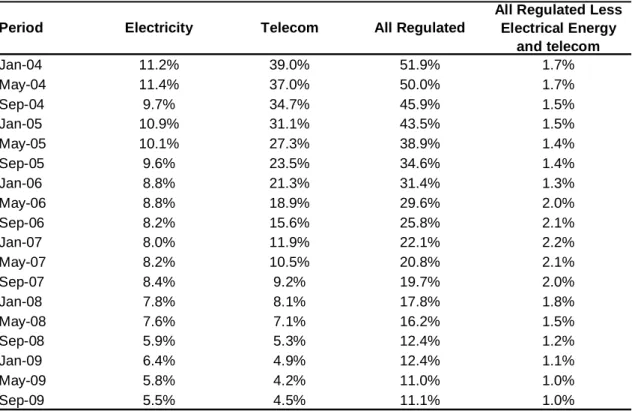
Table 1 shows the importance of regulated sectors for the sample. At the

beginning, the weight of telecommunications sector was the most important, featuring

nearly 39.0% while the total number of regulated sectors was 51.9% in the first quarter

of 2004. In the following periods, regulated sectors weight has been decreasing and in

September 2009 its participation in the sample was only 11.0% of the total, with the

telecommunications sector around 4.5% market share.

The Random-Effect panel data is used because to verify whether the betas of

regulated sector vary independently of other sectors. That is why I use time (or month)

and equities controls, which are taken into account in the estimation of the variance

and covariance matrix.

The test of Peltzman model in this environment is nothing more than verifies the

significance of the following null hypothesis:

H0: βregulated sector = βunregulated – There is regulatory risk

Ha: βregulated sector < βunregulated – There is no regulatory risk

... (7)

Equivalently we can test whether the parameter γ1 is greater than zero, i.e.:

H0: γ1 = 0 – there is regulatory risk associated with the sector;

Ha: γ1 < 0 - there is no regulatory risk associated with the sector.

... (8)

In theory, regulated sectors must have betas lower than unregulated sectors.

Therefore, comparing one sector with other regulated sectors as part of the control

group would facilitate the acceptance of the null hypothesis. This can occur because

betas of the control group could be underestimated as they include other regulated

sectors.

To address these possible distortions, the tests either for electricity and

telecommunications sectors take into account only unregulated sectors. For example,

(20)

telecommunications, the water utilities, gas distribution and the Road Concessions.

The same goes for the telecommunications sector, which exclude all the other three

sectors, in addition to electricity.

Period Electricity Telecom All Regulated

All Regulated Less Electrical Energy

and telecom

Jan-04 11.2% 39.0% 51.9% 1.7%

May-04 11.4% 37.0% 50.0% 1.7%

Sep-04 9.7% 34.7% 45.9% 1.5%

Jan-05 10.9% 31.1% 43.5% 1.5%

May-05 10.1% 27.3% 38.9% 1.4%

Sep-05 9.6% 23.5% 34.6% 1.4%

Jan-06 8.8% 21.3% 31.4% 1.3%

May-06 8.8% 18.9% 29.6% 2.0%

Sep-06 8.2% 15.6% 25.8% 2.1%

Jan-07 8.0% 11.9% 22.1% 2.2%

May-07 8.2% 10.5% 20.8% 2.1%

Sep-07 8.4% 9.2% 19.7% 2.0%

Jan-08 7.8% 8.1% 17.8% 1.8%

May-08 7.6% 7.1% 16.2% 1.5%

Sep-08 5.9% 5.3% 12.4% 1.2%

Jan-09 6.4% 4.9% 12.4% 1.1%

May-09 5.8% 4.2% 11.0% 1.0%

Sep-09 5.5% 4.5% 11.1% 1.0%

Source: BM&FBovespa.

Table 1: Electricity, Telecommunications and All Regulated Sectors dummies as percentage of the sample

I consider the BM&FBovespa criteria for Ibovespa, that is it represents a liquidity participation. The Electricity and Telecommunications sectors lost weight in the sample systematically during almost the entire period, which reduced the contribution of the regulated sectors in the Brazilian market. On the other hand, the other regulated industries have their weight increased, such as Gas Distribution, Road Concessions and Water Utilities.

3.4. EVENT STUDY FOR REGULATED SECTORS

In the second case, I consider only regulated sector stocks. The equation to be

estimated, therefore, is very similar to that of the first case and also I used the same

Random-Effect panel data method. However, the dummy variable in this case is

defined as a period around the ad hoc change in regulation for the two sectors

independently, that is electricity and telecommunications sectors:

t i i

t Event t

i, 0 1

D

2,

TimeContro

ls

3,

EquitiesCo

ntrols

v

,

ˆ

₌

_γ

₊

_γ

₊

_γ

₊

_γ

₊

β

... (9)

Where γ0, γ2,t and γ3,i are similar to those used to compare betas across sectors. In

(21)

assumes value one if the period belongs to the interval between two months before

and two months after regulatory event (in a total of five months) and zero otherwise. I

considered one event for electricity, the New Electricity Regulatory Framework, and

two for telecommunications sector: The New Text to Concession Contracts4 and The

New Maximum Rates of Remuneration that a telecom operator raises by receiving a

call from another operator5. These are represented in Table 2.

To verify that regulation change is associated to regulatory risk, it is necessary to

reject the null hypothesis that this event is not significant, i.e.:

H0: γ1 = 0 – there is regulatory risk associated with the sector;

Ha: γ1 < 0 - there is no regulatory risk associated with the sector.

... (10)

The disclaimer applied to the previous case that it should exclude regulated sectors

in the control group does not apply here because I consider the impact of regulation

change in the same sector.

4

http://www.anatel.gov.br/Portal/verificaDocumentos/documento.asp?numeroPublicacao=56441&assuntoPublicacao=An atel%20aprova%20os%20novos%20Contratos%20e%20o%20PGMQ%20do%20STFC%20%20&caminhoRel=null&filtr o=1&documentoPath=biblioteca/releases/2003/release_18_06_2003(4).pdf;

5

(22)

Sector Date New Regulation

Electricity March-16, 2004

President of the Republic signed the laws 10,847 and 10,848 for the new regulatory framework for Brazilian Electricity Sector. The Law number 10,847 authorized the creation of the Energy Research Company - EPE, while the Law 10,848 has established the new negotiation model for electricity.

June-18, 2003

New text of concession contracts. New contracts have a new index, called the Telecommunications Sector Index (IST), which replaces the IGP-DI and which is composed by several indexes (already existing). There are other measures, like the free access to the list of subscribers and the portability of phone numbers (Anatel, 2003).

December-20, 2005

New maximum rates of return that a telecom operator charge by receiving a call from another operator. In 2006, the value of the fee LAN will be 50% of the minutes and it would reduced to 40% by 2007. Since 2008, the value is based on the concessionaires costs (Anatel, 2005).

Source: Aneel and Anatel.

Table 2: Dates of Major Recent Changes in Legislation in the Electricity and the Telecommunications Sectors

Telecom

4. DATA BASE CONSTRUCTION AND VARIABLE SELECTION

4.1. DATA SOURCE

The data that I use can be grouped in three set of variables: the equity prices6, the

market portfolios and the risk free rates.

The equity prices are obtained directly from Bloomberg. For the market portfolios, in

turn, I considered two indexes both measured in Brazilian currency Real (BRL). The

first one is the Bovespa Index (Ibovespa) obtained from Bloomberg (ticker IBOV

INDEX). It is the most important market portfolio of the country and is the predominant

benchmark for much of the local equity mutual funds. It comprises the most traded and

liquid stocks in the Bolsa de Valores de São Paulo and its composition is updated each

third of the year.

The MSCI Brazil is used for robustness and is also obtained from Bloomberg (ticker

MXBR Index). It has a number of advantages over other indexes. First, the MSCI gives

6

(23)

greater weight to larger companies by market value. Theoretically this measure should

correlate more with the GDP. The Ibovespa, on the other hand, gives greater weight to

the most liquid stocks. Second, the MSCI does not take into account related companies

such as holdings and also facilitates comparison with other markets because it is

calculated by a common methodology. Finally, the shares in the MSCI Brazil represent

a maximum of 30% of the index7.

For the risk free rate, I use the main benchmark of the Brazilian market, the

Certificados de Depósitos Interbancários (CDI). It is also obtained from Bloomberg,

which provides an index of accumulated returns (ticker BZACCETP Index)8. CDI is

similar to the London Interbank Offering Rates (LIBOR) system, but it is an overnight

index and has been the most important benchmark for the Brazilian fixed income

markets for the last years.

Despite a well-developed financial system, the Brazilian financial system still has

remnants of more interventionist eras as the significant amount of credit directed by the

government and a set of interest rates for special funding targeted to such activities as

home acquisition, long-term business investment that eventually can affect the results

in tests of regulatory risk. For robustness I use three other benchmarks, the Reference

Rate (TR), the return of on passbook savings accounts (Cadernetas de Poupança, or

Poupança) and the long-term interest rate (TJLP), the reference rate lent by the

National Development Bank (BNDES). All data are from the Central Bank of Brazil9.

The TR is based on a monthly weighted average of fixed rate time deposits of a

certain number of financial institutions that is used in some investments. Passbook

savings accounts (Poupança) are deposits widely used by Brazilian families (workers).

These funds are deposited in financial institutions, remunerated at a rate of 6.0% per

year plus the reference rate (TR). Funds from these accounts finance the acquisition of

residential property. The TJLP is the interest rate that the BNDES charges on loans to

7

The Petrobrás shares are an example of such concentration in Ibovespa. The combined participation of all their shares (ON and PN, for instance) account for more than 16% of the Ibovespa’ weight by September, 2007;

8_{To obtain the accumulated returns, Bloomberg calculates a CDI return index accruing the rates in a daily basis through} the following specification:

12 1 252

100 1 1 100

   

   

   

 

+ +

= t

t

CDI X

IndexCDI ,

(24)

companies and serves as a reference for all directed credit. By October, 2009 this rate

stood at 6.5% per year10.

All rates used so far are backward looking, when in practice we know that investors

generally anticipate the movements of market interest rates. Therefore, I also use for

robustness the swap rate between the fixed and floating rate for one year known as the

Pré-DI swap for 360 days (Swap 360D), which is a forward looking benchmark. This

rate is also obtained from the Central Bank of Brazil.

4.2. PROCEDURE TO CALCULATE RETURNS AND ESTIMATION WINDOWS

I use end-of-month closing prices and rates for the period from January, 1999 until

the end of October, 2009.

For equities and market portfolios as the Ibovespa and MSCI Brazil, the return to

asset i at time t = 1,..., N,(Ri,t), is defined as:













=

−1

, ,

,

ln

t i

t i t

i

P

R

... (11)

where Pi,t is the price of asset i at time t.

Most of the risk free benchmarks used in this work are expressed in accumulated

monthly returns that have the advantage of adjusting for business days and for

changes in interest rates in the midterm. This is the case of TR, TJLP and Poupança,

where monthly returns come from the Central Bank of Brazil. Since I use monthly data

for these three risk free benchmarks (Rf,t) they can be represented by logarithmic form

(12):

(

t

)

t

f i

R , ₌ln 1₊ ... (12)

where it represents the accumulated monthly returns of TR, TJLP and Poupança at

time t.

For the risk free rate CDI, the most important fixed income benchmark in Brazilian

market, Bloomberg provides an index of accumulated returns. In this case, the

10

(25)

logarithmic return is obtained using the same procedure for equities return according to

Equation (11).

For the Swap 360D, considering its forward looking nature and since its given

yearly the risk free rate return at month t, Rf,t is:

(

)

12 1 ln

,

t t

f

i

R ₌ + ... (13)

Brazilian equity market liquidity is increasing as a result of a stable macroeconomic

environment and also and it is gaining importance in the international arena. However,

the liquidity was quite poor in the recent past and concentrated in few companies,

mainly large caps. Also, equity prices are affected by macroeconomic factors, for

instance the 2002 pre-election crisis, that affected small companies’ stock performance

disproportionately. For this reason I use the most liquid stocks, that is, equities that in

each period are part of the Ibovespa index.

As that Ibovespa’s implied portfolio is updated every four months, I update the

shares in the portfolio accordingly.

For historical reasons, the Brazilian equity market has a high proportion of

preferred shares compared to common stocks. The preferred stocks have preference

in the dividends distribution, but are nonvoting shares. Ordinary shares have voting

rights but do not have preference on the distribution of dividends. In order to not double

count and avoid over-representation of one company, less liquid stocks – whether

ordinary or preferred stock – are excluded from the sample if both belong to the

Ibovespa.

Another characteristic of the theoretical portfolio composition is that each stock

needs to be traded in at least in 48 of the 60 previous trading months (or 80% of the

time). For this, I consider January, 2004 as the first Ibovespa portfolio. Those that do

not satisfy this condition are excluded from the estimations. A list of all the shares used

in this paper as well as descriptive statistics such as mean and variance of returns can

(26)

4.3. DESCRIPTIVE STATISTICS OF THE SAMPLE

The purpose of this Section is to provide details about the characteristics of each of

the assets used, i.e. shares, market portfolios, risk free assets as well as sectorial

benchmarks for electricity and telecommunications.

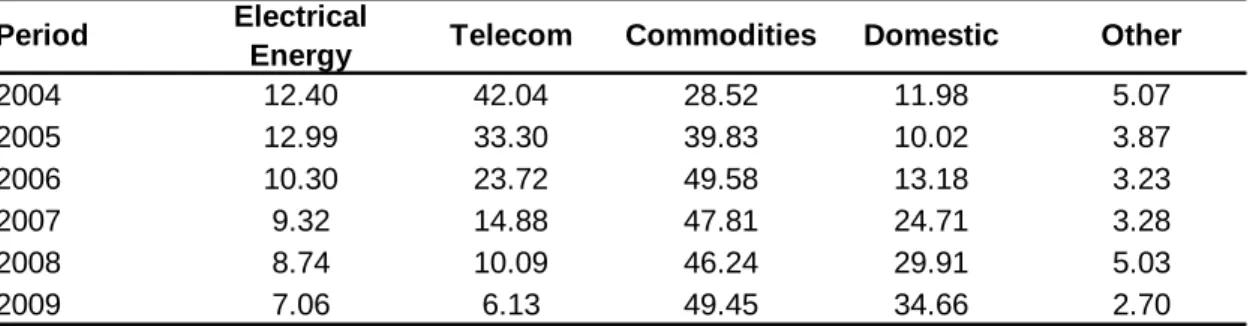
Table 3 shows the evolution of the Ibovespa portfolio since 2004. There are two

major changes in composition. The first one was that telecommunications fell in

importance compared to other sectors, most notably relative to commodities such as

mining, oil, gas and steel. Currently, a new trend in the stock market is underway with

the percentage of commodity sectors shrinking in favor of those more focused on

domestic market, i.e. the composition of the index is starting to better reflect the actual

economy.

One question that arises is whether the results obtained according to Section 3 are

caused by sample composition changes as represented by Table 3. For robustness, I

run the same regressions, but at the sectorial level considering the MSCI Brazil sectors

that controls for sample variation. The results are shown in Appendix A8 for sectors

comparison and A9 is for event study and they are the same comparing to those of the

main part of the Paper.

The distribution of individual equities returns is detailed in Table 4. On average, the

annualized monthly return of all stocks together is 19.5%, with an average standard

deviation of 48.8%.

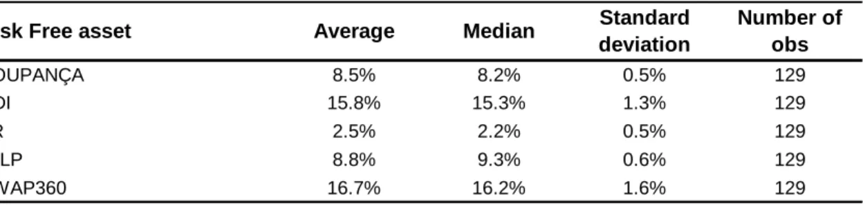
With regard to risk free assets used in this paper, Table 5 shows that subsidized

financing instruments have the worst performance, with TR – linked instruments putting

in the worst performance of all11. Its average annualized monthly return from January,

1999 through October, 2009 is 2.5%. TR return is only slightly outdone by Poupança

and TJLP-linked investment. Poupança averaged an annualized monthly return of

8.5%, and while TJLP-linked averaged 8.8%. The volatility of those instruments, on the

other side, is very small. TR and Poupança have a standard deviation of 0.5% per year

and TJLP 0.6%.

Conversely, the interbank market rates - CDI - and Swap 360D are those that

provided the greatest gains accrued for the period. The CDI rate has lower market risk

than Swap 360D because it represents the interest paid overnight, that is, its duration

11

(27)

is only one day (Table 4). CDI has an annualized monthly return of 15.8% and a

standard deviation of 1.3%, but the outlook for the coming years is that this rate will fall

as a result of persistent inflation stabilization in Brazil over the last two decades.

The Swap 360D, in turn, has the highest returns since January, 1999, averaging

16.7% per month annualized. Volatility, on the other hand, is the highest among fixed

income benchmarks, reaching 1.6% per month annualized. This strengthens the

previous perception that the Swap 360D may be the best risk free asset by taking into

account the forward looking nature of interest rates.

The details of the market portfolios are shown in Table 6. The MSCI Brazil seems

to have performed better than the Ibovespa. The Morgan Stanley index has higher

monthly returns: on average, 18.9% per year against 18.8% of Ibovespa with lower

volatility. The standard deviation of its returns for the entire period is 26.4% per month

annualized, while the standard deviation for the main stock index of the Brazilian

market is 28.9%.

Table 7 shows the risk and return for electricity and telecommunications

benchmarks in Brazil. For the electricity sector, I use the Electricity Index (IEE) and the

MSCI Utilities, both measured in BRL. The IEE has a 26.0% return per month

annualized, higher than the MSCI Utilities with 10.3%.The MSCI Utilities, however, has

lower volatility at 34.5% per month compared to the IEE whose volatility is 40.4%.

Table A3 in the Appendix details the composition of IEE from September, 09 to

December, 09 while Table A4 shows the composition of the MSCI Utilities for October,

09.

For telecommunications benchmarks, I use the Telecommunications Index (ITEL)

and the MSCI Telecommunications Services, both measured in BRL. The MSCI sector

benchmark shows the worst results. One explanation may be the inclusion of fewer

shares as opposed to ITEL. This may justify the MSCI’s greater volatility, with a

standard deviation 29.2% per month annualized, than the ITEL, with volatility of 32.6%

(Table 6). Table A5 in the Appendix details the composition of the ITEL from Sep-09 to

Dec-09 while Table A6 shows the composition of the MSCI Telecommunications

(28)

Period Electrical

Energy Telecom Commodities Domestic Other

2004 12.40 42.04 28.52 11.98 5.07

2005 12.99 33.30 39.83 10.02 3.87

2006 10.30 23.72 49.58 13.18 3.23

2007 9.32 14.88 47.81 24.71 3.28

2008 8.74 10.09 46.24 29.91 5.03

2009 7.06 6.13 49.45 34.66 2.70

Source: BM&FBovespa.

Table 3: Evolution of the selected sectors weight in the Ibovespa

In percentage considering the first composition of the year

(i) Electricity and Telecommunications follows the classification of the Bovespa. For the sector classification of Commodities and Domestic, I also used the following sectors based on the Brazilian Stock Exchange criteria - Commodities: Oil and Gas, Steel and Metallurgy, Wood and Paper, Chemical and Petrochemical and Mining. Domestic: Banks and Financial Intermediaries, Transportation, Consumer Staples, Consumer Discretionary and Real State.

(29)

Company Average Median Standard deviation

Number of obs

ACES4 31.4% 11.5% 42.5% 111

ALLL11 12.4% 7.3% 40.5% 55

AMBV4 24.1% 26.6% 27.7% 129

ARCE3 43.1% 45.3% 43.3% 101

ARCZ6 1.2% -2.4% 52.3% 129

BBAS3 24.1% 24.2% 41.6% 129

BBDC4 24.4% 23.4% 37.2% 129

BRAP4 16.8% 22.1% 42.2% 110

BRKM5 17.3% 0.7% 49.3% 129

BRTO4 10.1% 9.4% 37.8% 129

BRTP4 2.9% -14.2% 34.9% 129

BTOW3 21.7% 28.6% 54.7% 55

CCRO3 26.4% 21.0% 41.5% 93

CESP6 5.6% 52.9% 61.0% 39

CGAS5 17.6% 8.2% 40.3% 129

CLSC6 12.0% 17.1% 35.7% 129

CMET4 61.2% 55.2% 40.0% 88

CMIG4 13.2% 25.9% 35.7% 129

CPFE3 11.7% 0.4% 24.8% 61

CPLE6 12.0% 15.4% 37.8% 129

CRTP5 17.9% 21.0% 60.7% 77

CRUZ3 16.6% 17.9% 31.0% 129

CSNA3 32.1% 48.7% 49.1% 129

CSTB4 42.9% 37.6% 48.1% 82

CYRE3 41.3% -19.6% 66.8% 51

DURA4 21.5% 14.4% 37.9% 129

EBTP4 -4.2% 8.6% 66.8% 129

ELET6 5.0% 11.6% 40.5% 129

ELPL5 12.5% 10.6% 51.6% 129

ELPL6 10.8% 5.2% 30.3% 38

EMBR3 -0.7% 11.4% 69.8% 129

EMBR4 108.0% 17.2% 290.1% 90

GGBR4 34.8% 30.8% 45.0% 129

GOAU4 36.2% 34.0% 41.6% 129

GOLL4 -6.9% 4.0% 50.3% 64

ITAU4 25.2% 23.3% 34.3% 129

ITSA4 26.7% 25.5% 32.9% 129

KLBN4 22.0% 11.2% 38.7% 129

LAME4 39.1% 49.5% 60.4% 129

LIGT3 1.5% -4.4% 50.1% 129

LREN3 46.7% 15.9% 75.5% 111

NATU3 24.1% 38.5% 29.3% 65

NETC4 -2.7% 11.3% 80.1% 128

PCAR4 15.3% 17.7% 35.6% 129

PETR4 28.1% 24.6% 37.4% 129

PRGA3 26.3% 26.0% 39.3% 129

PTIP4 20.2% 26.0% 37.2% 108

RDCD3 -9.1% -21.6% 31.6% 21

RSID3 18.7% 7.4% 69.9% 124

SBSP3 13.5% -3.6% 42.1% 129

SDIA4 21.0% 31.8% 43.0% 128

TAMM4 19.2% -2.1% 67.9% 70

TBLE3 27.8% 16.6% 41.2% 129

TCOC4 24.4% 19.9% 46.0% 86

TCSL4 2.5% 3.0% 48.3% 129

TLCP4 -0.4% 0.0% 64.5% 86

TLPP4 1.8% -3.0% 32.3% 129

TMAR5 6.9% 5.7% 39.1% 129

TMCP4 13.1% 7.8% 42.7% 128

TNEP4 18.7% 32.6% 54.7% 69

TNLP4 7.9% 14.7% 37.5% 129

TRPL4 29.8% 44.7% 44.2% 123

UBBR11 19.7% 28.5% 43.9% 122

UGPA4 13.8% 16.2% 30.2% 120

USIM5 33.8% 60.7% 51.3% 129

VALE5 25.7% 18.4% 33.1% 129

VCPA4 16.4% 25.8% 47.3% 127

VIVO4 -10.9% 1.2% 57.6% 129

(30)

Risk Free asset Average Median Standard deviation

POUPANÇA 8.5% 8.2% 0.5% 129

CDI 15.8% 15.3% 1.3% 129

TR 2.5% 2.2% 0.5% 129

TJLP 8.8% 9.3% 0.6% 129

SWAP360 16.7% 16.2% 1.6% 129

Source: Bloomberg and Central Bank of Brazil.

Table 5: Descriptive Statistics of Risk Free Assets Monthly Returns - Annualized From February, 1999 up to October, 2009

Market Portfolio Average Median Standard

deviation

IBOVESPA 18.8% 23.0% 28.9% 129

MSCI BR 18.9% 23.5% 26.4% 129

Source: Bloomberg.

Table 6: Descriptive Statistics of Market Portfolios Monthly Returns - Annualized From February, 1999 up to October, 2009

Benchmark Average Median Standard

deviation

IEE (BRL) 26.0% 23.9% 40.4% 129

MSCI UTILITIES (BRL) 10.3% 14.2% 34.5% 129

ITEL (BRL) 3.1% 3.1% 29.2% 118

MSCI TELECOM (BRL) 2.9% 2.2% 32.6% 129

Source: BM&FBovespa and Bloomberg.

(31)

5. RESULTS

5.1. ARE THE BETAS OF REGULATED SECTORS LOWER THAN THOSE OF OTHER SECTORS?

In theory, if there is no regulatory risk, betas of regulated sectors should be lower

than those without regulation. This is not the case, however, in electricity,

telecommunications and all regulated sectors in Brazilian market, including water

utilities, road concessions and gas distribution.

The econometric tests in general accept the hypothesis that the betas of regulated

sectors are similar to the other sectors. In fact, the tests show that their betas are even

higher compared to unregulated sectors for the period from February, 1999 through

October, 2009.

Table 8 summarizes the results obtained for the electricity sector from the

regressions based on Equation (5). For robustness, I used two market portfolios, the

Ibovespa and the MSCI Brazil, and five risk free assets, CDI, Poupança, Swap 360D,

TJLP and TR (10 regressions). The parameters associated with time and equities

controls are not reported.

When both the Ibovespa and MSCI Brazil are used as market portfolios, the

majority of coefficients associated with electricity sector are positive and significant at a

1% level. Only one regression showed otherwise. When I used the TR as risk free

asset and the MSCI Brazil as market portfolio, the coefficient associated with the beta

parameter was negative and significant at 1%.

Even with this exception, probably related to the fact that TR is a subsidized rate,

the results are robust to changes in risk free assets. The parameter associated with the

electricity dummy range from 0.495 when CDI is the risk free asset and Ibovespa is the

market portfolio is to 0.560 when Swap Pre-DI is risk free rate. The market portfolio in

this last case is also the Ibovespa.

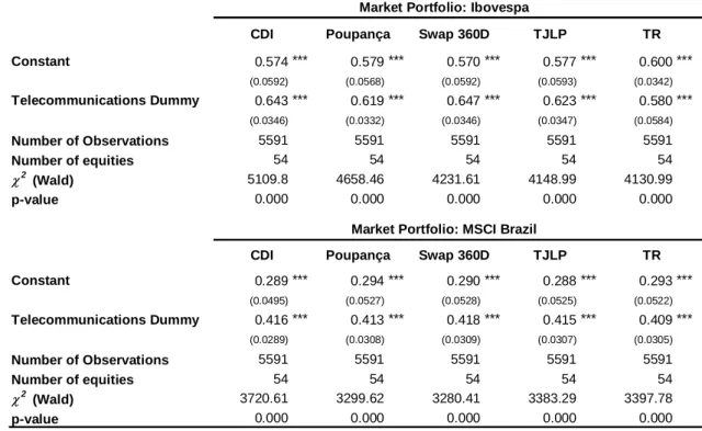
Table 9 presents the results obtained using the same procedure for

telecommunications sector. The difference is that the dummy variable assumes value

(32)

Constant 0.593 *** 0.595 *** 0.594 *** 0.598 *** 0.605 ***

(0.0488) (0.0486) (0.0495) (0.0486) (0.0476)

Electricity Dummy 0.495 *** 0.556 *** 0.560 *** 0.555 *** 0.557 ***

(0.04740 (0.0473) (0.0481) (0.0472) (0.0462)

Number of Observations 5024 5024 5024 5024 5024

Number of equities 50 50 50 50 50

χ2 (Wald) 6248.61 5109.39 4990.72 5074.62 5097.6

p-value 0.000 0.000 0.000 0.000 0.000

Constant 0.308 *** 0.313 *** 0.311 *** 0.310 *** 0.321 ***

(0.0380) (0.0379) (0.0379) (0.0374) (0.0367)

Electricity Dummy 0.534 *** 0.529 *** 0.533 *** 0.531 *** -0.090 ***

(0.0369) (0.0368) (0.0369) (0.0364) (0.0295)

χ2 (Wald) 4700.47 4524.95 4652.57 4733.85 4848.94

p-value 0.000 0.000 0.000 0.000 0.000

* Statistically significant at 10%. ** Statistically significant at 5%. *** Statistically significant at 1%.

Table 8: Are the betas of the regulated sectors lower than those of other sectors?

Market Portfolio: MSCI Brazil

CDI Poupança Swap 360D TJLP TR

Market Portfolio: Ibovespa

CDI Poupança

This Table presents the results of the regressions:βit est₌_γ

0+γ1Di+γ2tTime Controlst+γ3iEquities Controls+vitestimated from February, 1999

up to October, 2009.

Electricity

Swap 360D TJLP TR

This equation was estimated using the Random Effect panel. The dependent variablesβit

est_{are the CAPM betas for each stock estimated in the}

first step by Kalman Filter.γ0is the parameter associated with the constant term,γ1is the parameter associated with the dummy variable that

assumes value one if the equity belongs to the Electricity Sector and zero otherwise,γ2t is the t -dimensional parameter vector associated with a

time-trend,γ3tis the i -dimensional parameter vector associated with equities controls and vit are the erratic term. The dummy controls for time

and equities have not been reported. The values in brackets are standard deviations associated with the coefficients.The table is divided in two parts: the first shows the results using the betas estimated in the first step considering the Ibovespa as the market portfolio, while in the second the betas were estimated using the MSCI Brazil. For each of these market portfolios, we used five risk free assets for robustness, the CDI, the Poupança, the Swap 360D, the TJLP and the TR, respectively.

The results are similar to those obtained for electricity sector. That is, the

coefficients associated with dummy variable for telecommunications sector are all

positive and significant when using both the Ibovespa index and the MSCI Brazil as

market portfolios. Unlike for the electricity sector, there are no negative significant

betas, further evidence of regulatory risk.

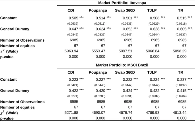
Finally, Table 10 shows the tests for all regulated sectors together, which includes,

besides electricity and telecommunications, gas distribution, road concessions and

water utilities. The coefficients associated with the dummies are all positive and

(33)

Constant 0.574 *** 0.579 *** 0.570 *** 0.577 *** 0.600 ***

(0.0592) (0.0568) (0.0592) (0.0593) (0.0342) Telecommunications Dummy 0.643 *** 0.619 *** 0.647 *** 0.623 *** 0.580 ***

(0.0346) (0.0332) (0.0346) (0.0347) (0.0584)

χ2 (Wald) 5109.8 4658.46 4231.61 4148.99 4130.99

p-value 0.000 0.000 0.000 0.000 0.000

Constant 0.289 *** 0.294 *** 0.290 *** 0.288 *** 0.293 ***

(0.0495) (0.0527) (0.0528) (0.0525) (0.0522) Telecommunications Dummy 0.416 *** 0.413 *** 0.418 *** 0.415 *** 0.409 ***

(0.0289) (0.0308) (0.0309) (0.0307) (0.0305)

χ2 (Wald) 3720.61 3299.62 3280.41 3383.29 3397.78

p-value 0.000 0.000 0.000 0.000 0.000

Telecommunications

This Table presents the results of the regressions:βitest=γ0+γ1Di+γ2tTime Controlst+γ3iEquities Controls+vitestimated from February, 1999 up to

October, 2009.

This equation was estimated using the Random Effect panel. The dependent variablesβitestare the CAPM betas for each stock estimated in the first

step by Kalman Filter.γ0is the parameter associated with the constant term,γ1is the parameter associated with the dummy variable that assumes

value one if the equity belongs to the Telecommunications Sector and zero otherwise,γ2tis the t -dimensional parameter vector associated with a

time-trend,γ3tis the i -dimensional parameter vector associated with equities controls and vitare the erratic term. The dummy controls for time and equities

have not been reported. The values in brackets are standard deviations associated with the coefficients.The table is divided in two parts: the first shows the results using the betas estimated in the first step considering the Ibovespa as the market portfolio, while in the second the betas were estimated using the MSCI Brazil. For each of these market portfolios, we used five risk free assets for robustness, the CDI, the Poupança, the Swap 360D, the TJLP and the TR, respectively.

In all regressions I use month and equities controls. Consequently, specific effects

associated with period of time or that have affected only the beta of a specific share in

(34)

Constant 0.505 *** 0.514 *** 0.501 *** 0.508 *** 0.515 ***

(0.0532) (0.0511) (0.0533) (0.0529) (0.0518)

General Dummy 0.647 *** 0.624 *** 0.652 *** 0.628 *** 0.605 ***

(0.0346) (0.0332) (0.0347) (0.0344) (0.0337)

χ2 (Wald) 5963.94 5553.47 5097.51 5066.84 5098.29

p-value 0.000 0.000 0.000 0.000 0.000

Constant 0.223 *** 0.227 *** 0.222 *** 0.224 *** 0.237 ***

(0.0421) (0.0443) (0.0447) (0.0442) (0.0437)

General Dummy 0.422 *** 0.420 *** 0.424 *** 0.422 *** 0.415 ***

(0.0274) (0.0288) (0.0291) (0.0287) (0.0284)

χ2 (Wald) 5271.88 4690.07 4679.74 4789.93 4813.44

p-value 0.000 0.000 0.000 0.000 0.000

All Regulated Sectors

This Table presents the results of the regressions:βitest=γ0+γ1Di+γ2tTime Controlst+γ3iEquities Controls+vitestimated from February, 1999 up to

October, 2009.

This equation was estimated using the Random Effect panel. The dependent variablesβitestare the CAPM betas for each stock estimated in the first

step by Kalman Filter.γ0is the parameter associated with the constant term,γ1is the parameter associated with the dummy variable that assumes

value one if the equity belongs to All Regulated Sector and zero otherwise,γ2tis the t -dimensional parameter vector associated with a time-trend,γ3t is

the i -dimensional parameter vector associated with equities controls and vitare the erratic term. The dummy controls for time and equities have not

been reported. The values in brackets are standard deviations associated with the coefficients.The table is divided in two parts: the first shows the results using the betas estimated in the first step considering the Ibovespa as the market portfolio, while in the second the betas were estimated using the MSCI Brazil. For each of these market portfolios, we used five risk free assets for robustness, the CDI, the Poupança, the Swap 360D, the TJLP and the TR, respectively.

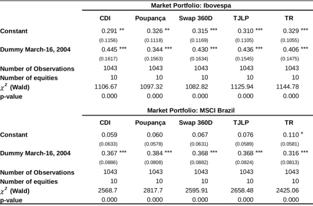
5.2. ARE THE BETAS OF REGULATED SECTORS AFFECTED BY ADHOC REGULATION CHANGES?

If an unexpected change in regulation would reduce the uncertainty about

companies’ cash flow, the betas around the period of regulation change should fall

compared to other periods. If a change in legislation does not change or even increase

the uncertainty of investors, variability of returns should increase and betas should rise

for that period.

It seems to be the case when the Brazilian government launched a new regulatory

framework for electricity sector, on March 16, 2004. The estimates show evidence of

Essays on regulatory risk issues

School of Business and Economics

Getulio Vargas Foundation

Thesis submitted to the School of Public Administration and Government of

Getulio Vargas Foundation as partial requirement for obtaining the Degree of

Doctor in Public Administration

Essays on Regulatory Risk Issues

São Paulo

School of Business and Economics

Getulio Vargas Foundation

Thesis submitted to the School of Public Administration and Government of

Getulio Vargas Foundation as partial requirement for obtaining the Degree of

Doctor in Public Administration

Essays on Regulatory Risk Issues

São Paulo

Contents

General Comments

Regulatory Risk in the Securities Markets: a CAPM

Model Approach to Regulated Sectors in Brazil

June, 20 - 2010

[

R

R

]

E

−

=

λ

β

(

)

(

)

R

R

R

var

,

cov

=

β

[

R

R

]

E

−

(

)

R

R

R

R

−

=

α

+

β

−

+

ε

(

)

R

R

R

R

−

=

β

−

+

ε

α

π

β

ν

β

=

+

₋

₌

₋

₌

₊

₋

₊

₋

₌

₋

₊

₌

₊

₊

₌

₌

_γ

₊

_γ

₊

_γ

₊

_γ

₊

₌

_γ

₊

_γ

₊

_γ

₊

_γ

₊