Projeto de redes de sensores sem fio heterogêneas utilizando os conceitos de redes small word

(1)

PEQUENO NO PROJETO DE TOPOLOGIAS

PARA REDES DE SENSORES SEM FIO

(2)

APLICAÇÃO DOS CONCEITOS MUNDO

PEQUENO NO PROJETO DE TOPOLOGIAS

PARA REDES DE SENSORES SEM FIO

HETEROGÊNEAS

Tese apresentada ao Programa de Pós--Graduação em Ciência da Computação do Instituto de Ciências Exatas da Universi-dade Federal de Minas Gerais como req-uisito parcial para a obtenção do grau de Doutor em Ciência da Computação.

Orientador: Antonio Alfredo Ferreira Loureiro

Co-Orientador: Raquel Aparecida de Freitas Mini

Belo Horizonte

(3)

APPLYING THE SMALL WORLD CONCEPTS

ON THE DESIGN OF HETEROGENEOUS

WIRELESS SENSOR NETWORKS TOPOLOGIES

Dissertation presented to the Graduate Program in Computer Science of the Fed-eral University of Minas Gerais in partial fulfillment of the requirements for the de-gree of Doctor in Computer Science.

Advisor: Antonio Alfredo Ferreira Loureiro

Co-Advisor: Raquel Aparecida de Freitas Mini

Belo Horizonte

(4)

!"#$%&#, '(&#)*+,"$%-#.%.

G948m Aplicação dos conceitos mundo pequeno no projeto de topologias para redes de sensores sem fio heterogêneas++ +

+++++++++++++'(&#)*+,"$%-#.%+!"#$%&#/+0+1)*%+2%3#4%&5)6+7899/ xvii, 97f. : il. ; 29cm

:);)+<$%"5%3($%=+0+Universidade Federal de Minas Gerais. Departamento de Ciência da Computação.

Orientador: Antônio Alfredo Ferreira Loureiro Coorientadora: Raquel Aparecida de Freitas Mini

1.+>%?@"5(AB%+C+:););. 2. Redes de computação– Teses. 3. D)$);+$)+;)&;%3);+;)?+E#%+– Teses.

I. Orientador. II. Coorientador. III. Título.

(5)

(6)

(7)

Uma Rede de Sensor Sem Fio (RSSF) considera um conjunto de nós homogêneos em termos de hardware. Entretanto, esse tipo de rede possui baixos limites de desem-penho em relação à latência durante a comunicação de dados. Outro modelo de RSSF, chamado de Redes de Sensores Sem Fio Heterogêneas (RSSFH), considera um conjunto de nós sensores heterogêneos em termos dehardware, especialmente em relação ao raio de comunicação e reservas de energia. Neste trabalho é proposto modelos baseados na teoria deSmall World no projeto de Redes de Sensores Sem Fio Heterogêneas. O primeiro modelo proposto considera o padrão de comunicação em RSSF na criação de atalhos direcionados ao nó monitor da rede com o objetivo de reduzir a latência na comunicação de dados. Os pontos finais desses atalhos são nós com maior capacidade de comunicação e reservas de energia para suportar a comunicação de longo alcance. O modelo proposto foi avaliado e foi verificado que o mesmo apresenta as mesmas carac-terísticas de redesSmall World (caminho médio mínimo e coeficiente de agrupamento) observadas nos modelos da literatura. Além disso, quando os atalhos são criados na direção ao nó monitor, depositando uma pequena quantidade de nós com maior ca-pacidade de hardware, o modelo proposto apresenta melhores características de redes

Small World e melhores tradeoffs entre latência e energia consumida durante a comu-nicação de dados quando comparado aos modelos da literatura. O modelo proposto também foi avaliado com relação à resiliência considerando falhas gerais e específicas e, em ambos os casos, o modelo proposto se mostrou mais robusto e apresenta uma baixa degradação da comunicação de dados na presença de falhas nos nós. Entretanto, a co-municação de longo alcance entre os nós com maiores capacidade de coco-municação causa uma alta interferência no canal sem fio. Para isso, nós apresentamos um modelo para criação de RSSFH que utiliza múltiplas interfaces sem fio e a capacidade de utilização de múltiplos canais de comunicação da camada MAC para reduzir as colisões durante a comunicação de dados. Resultados de simulação mostraram que quando os atalhos são direcionados ao nó monitor e assinalados a diferentes canais de comunicação sem fio, as colisões são reduzidas e, por conseguinte, a latência na comunicação de dados é

(8)

três topologias para prover qualidade de serviço em RSSFH. Cada topologia possui o seu objetivo em relação à latência e energia consumida durante a comunicação de da-dos. Resultados de simulação mostraram que a utilização das topologias doframework

proposto reduz o consumo de energia e a latência quando comparado as topologias utilizadas na literatura para prover qualidade de serviço em redes de sensores sem ﬁo heterogêneas.

Palavras-chave: Redes de Sensores Sem Fio, Redes de Sensores Sem Fio Het-erogêneas, Comunicação de Dados, Redes Small World, Qualidade de Serviço.

(9)

A typical Wireless Sensor Network (WSN) assumes a homogeneous set of nodes in terms of capabilities. However, this kind of network suffers from poor fundamen-tal limitations of latency during the data communication. Another model of WSN assumes a heterogeneous set of nodes with different capabilities (especially in terms of communication range and energy reserves) called Heterogeneous Sensor Networks (HSN). In this work, we propose small world models to design Heterogeneous Sensor Networks (HSNs). The first model takes into account the communication pattern of this network to create shortcuts directed to the monitoring node, decreasing the data communication latency. The endpoints of these shortcuts are nodes with more powerful communication range and energy reserves to support the long communication range. We evaluate the proposed model and show that they present the same small world fea-tures (average path length and clustering coefficient) observed in the literature models. When the shortcuts are created toward the sink node, with a few number of powerful sensors, the network presents better small world features and interesting tradeoffs be-tween energy and latency in the data communication when compared to the literature model. Also, we evaluate the resilience of the proposed model considering general and specific failures and, in both cases, the proposed model is more robust and presents a graceful degradation of the network latency, which shows the resilience of those models. However, the long range communication used to create a shortcut causes a high inter-ference in the wireless channel. For this, we present a model that uses multi-interface and multi-channel capability of the MAC layer to reduce collisions during the data communication. Simulation results showed that when the shortcuts are directed to the sink node and assigned to a different wireless channel, collisions and latency are reduced. We also proposed a framework based on the small world concepts to design heterogeneous sensor networks with QoS. The framework uses three different topolo-gies to provide QoS in sensor networks. Each topology has its own objectives related to latency during communication and energy consumption. Simulation results showed that the proposed framework can reduce latency and energy consumption compared to

(10)

Keywords: Wireless Sensor Networks, Heterogeneous Sensor Networks, Data Com-munication, Small World Networks, Quality of Service.

(11)

1.1 Data Communication in WSN. . . 2

2.1 Example of graphs using the random rewiring technique . . . 13

2.2 Example of graphs using the random addition model . . . 14

2.3 Example of L-sensor and H-sensor . . . 19

3.1 Creation of shortcuts when the value of p changes in the random addition model . . . 23

3.2 Directed angulation toward the sink model . . . 24

3.3 Creation of shortcuts when the value of p changes in the TDASM model (φ= 30◦_{) . . . .} ₂₅

3.4 Small world features of the theoretical models . . . 31

3.5 Small world features of on-line models . . . 33

3.6 Latency in the data communication . . . 36

3.7 Latency in the data communication with ﬁve general failures. Figs (a)–(c) show the shortcuts in ORAM. Figs (d)–(f) show the shortcuts in ODASM 40 3.8 Latency in the data communication with general failures . . . 41

3.9 Latency in the data communication with speciﬁc failures (50% of H-sensors). Figs (a)–(c) show the shortcuts in ORAM. Figs (d)–(f) show the shortcuts in ODASM . . . 42

3.10 Latency in the data communication with speciﬁc failures . . . 43

4.1 Directed region to the sink node . . . 48

4.2 Directed Angulation toward the sink Model . . . 49

4.3 Small world features . . . 52

4.4 Number of collisions . . . 54

4.5 Data communication latency . . . 55

5.1 Framework topologies . . . 60

(12)

5.4 Small world features . . . 77

5.5 Comparison among the three topologies . . . 77

5.6 Number of components among the H-sensor network . . . 79

5.7 Latency evaluation . . . 80

(13)

3.1 Number of added links for all models when we change the probability of

shortcut addition . . . 32

3.2 Energy consumption and transmitted packets . . . 35

4.1 Number of collisions points . . . 53

5.1 Energy consumption in Joules. L (L-sensors) and H (H-sensors) . . . 82

(14)

1 ODASM algorithm . . . 29

2 Algorithm to create the homogeneous topology’s routing . . . 62

3 Algorithm to create the DASM topology’s routing . . . 64

4 Shortcut Creation of the DASM Tree model . . . 68

5 Algorithm to create the DASM Tree topology’s routing . . . 71

6 QoS Routing Algorithm . . . 73

(15)

Resumo vii

Abstract ix

List of Figures xi

List of Tables xiii

1 Introduction 1

1.1 Motivation . . . 1

1.2 Objectives . . . 3

1.3 Contributions of this Thesis . . . 5

1.4 Other Contributions . . . 7

1.5 Work Organization . . . 8

2 Background and Related Work 9 2.1 Background . . . 9

2.1.1 Complex Networks . . . 9

2.1.2 Small World Networks . . . 11

2.2 Related Work . . . 15

2.2.1 Small World in Wireless Networks . . . 15

2.2.2 Heterogeneous Sensor Networks . . . 17

2.3 Final Remarks . . . 20

3 Directed Angulation Toward the Sink Node 21 3.1 Shortcut Creation in Wireless Sensor Networks . . . 21

3.2 Theoretical Directed Angulation Toward the Sink Node . . . 23

3.3 On-line Model to Design HSNs . . . 26

3.4 Protocol Design of the On-line Model . . . 27

(16)

3.6.1 Scenarios . . . 30

3.6.2 Small World Features Evaluation . . . 30

3.6.3 Experimental Evaluation . . . 34

3.6.4 Experimental Evaluation in Potential Failure Scenarios . . . 37

4 Multi-Channel Multi-Interface Directed Angulation Toward the Sink Node 45 4.1 Introduction . . . 46

4.2 Shortcut Creation . . . 46

4.3 Channel Assignment . . . 48

4.4 Simulation Results . . . 50

4.4.1 Scenarios . . . 50

4.4.2 Small World Features Evaluation . . . 51

4.4.3 Collision Evaluation . . . 52

4.4.4 Latency Evaluation . . . 53

4.5 Related Work . . . 55

5 A Framework based on Small World Features to Design HSN Topologies with QoS 57 5.1 Introduction . . . 57

5.2 Framework Design . . . 59

5.2.1 Introduction . . . 59

5.2.2 Homogeneous Topology . . . 61

5.2.3 DASM Topology . . . 62

5.2.4 DASM Tree Topology . . . 64

5.3 Framework Instantiation . . . 72

5.4 Simulation Results . . . 73

5.4.1 Scenarios . . . 73

5.4.2 Methodology . . . 74

5.4.3 Small World Features . . . 75

5.4.4 Number of Connected Components . . . 78

5.4.5 Latency Evaluation . . . 78

5.4.6 Energy Evaluation . . . 81

(17)

6 Conclusion and Future Work 84

6.1 Summary of this Work . . . 84 6.2 Future Work . . . 85

Bibliography 87

(18)

Introduction

1.1 Motivation

Wireless sensor networks (WSNs) [Estrin et al., 1999; Intanagonwiwat et al., 2002; Pottie and Kaiser, 2000; Akyildiz et al., 2002] are composed of sensors nodes that collect data from the environment, where they are embedded and proceed to be processed and relayed to a monitoring node. This node often does not have resource restrictions and is responsible for collecting information about the network and sending control data to sensor nodes. Sensor nodes interconnected through wireless communication networks with the goal of performing any sensing task will improve how information is collected and processed. Wireless sensor networks need to carefully integrate functionalities traditionally considered to be separate to achieve maximum eﬃciency, with respect to energy consumption and management. Additionally, WSNs are evolving from simple data transportation networks to functionally rich distributed systems. Wireless sensor networks can be employed in the monitoring, tracking, coordination and processing of diﬀerent applications. For instance, sensors can be interconnected to monitor and control environmental conditions in a forest, ocean or planet.

Data communication in WSNs tends to be diﬀerent from “traditional” data net-works in such a way that the sink node is either the origin or the destination of a message, whereas in other networks data communication happens between arbitrary communicating entities. In this case, the data communication from the point of view of the communicating entities can be divided into two types, as depicted in Figure 1.1: from sensors to a monitoring node, and from a monitoring node to sensors. The ﬁrst one, called data collection (Figure 1.1(a)), is used to send the sensed data to a mon-itoring application. It is also used when sensor nodes have to send important control information to a monitoring node, such as their energy consumption. The second one,

(19)

called data dissemination (Figure 1.1(b)), is normally used when a monitoring node has to disseminate some information to sensor nodes. Reliable data dissemination is crucial when a monitoring node has to perform some speciﬁc activities, such as to disseminate an information that is important to all sensor nodes, change the operational mode of part or the entire network, activate/deactivate one or more sensors, and send queries or new interests to the network. The sink node may also wants to change the node duty cycle. Furthermore, data dissemination is fundamental to the basic operation of many protocols in WSNs such as identiﬁcation of multiple paths between sensor nodes and establishment and maintenance of routes.

(a) Data Collection (b) Data Dissemination

Figure 1.1. Data Communication in WSN.

A usual model of a WSN assumes a homogeneous set of nodes, i.e. all nodes have the same capabilities of memory, processing and communication range. How-ever, Gupta and Kumar [2000] and Yarvis et al. [2005] show that a homogeneous ad hoc network suﬀers from poor fundamental limits and network performance related to latency, throughput, etc. For instance, in a multi-hop homogeneous WSN, nodes close to the sink tend to spend a signiﬁcant amount of energy routing packets from other nodes, which can eventually lead to a disconnected topology.

(20)

neighbors while L-sensors have just a few.

Complex Networks [Newman, 2003; Watts, 2007; Kleinberg, 2008] are becom-ing more important to model a network that has certain non-trivial topological fea-tures [da F. Costa et al., 2007] as found in small world or scale free graphs. An important model of a complex network is the small world model [Watts and Strogatz, 1998; Amaral et al., 2005; Strogatz, 2001a], which presents desired characteristics for a computer network such as small average path length between pairs of nodes and high cluster coeﬃcient1

. The small average path length leads to a small data communica-tion latency and high values of clustering coefficient can improve the network resilience. In the context of a computer network, resilience means the capacity of a network to provide and maintain an acceptable quality of service (specified by the user and/or network designer) related to latency, energy consumption and others in the presence of faults [Menth and Martin, 2005]. Resilience is recognized as a fundamental attribute for truly effective use of wireless sensor networks.

In order to create a network with small world features, the designer should add a small number of long-range links, called shortcuts. In traditional networks, the goal of the shortcuts is to optimize the communication between pairs of nodes. However, in WSNs, data communication typically happens when the sink node wants to send a message to the sensor nodes (data dissemination), or when the sensor nodes send the sensed data to the sink node (data collection). Due to the speciﬁc communication pattern of wireless sensor networks, the goal of the shortcuts in such a network should be to optimize the communication between sink node and sensor nodes, instead optimizing the communication for any pairs of nodes. Thus, to improve the data communication in wireless sensor networks, the shortcuts should be created toward the sink node.

Also, when a WSN is modeled according to the small world concepts, the network becomes more robust to the presence of node failures due to the shortcut addition, i.e. the network becomes more resilient. In this case, the shortcuts may interconnect the remaining nodes, keeping alive the data communication in the network [Albert et al., 2000].

1.2 Objectives

The main goal of this proposal is to design heterogeneous wireless sensor networks based on the small world models to improve data communication in wireless sensor

1

(21)

network. In this way, when a network exhibits small world features, the following issues can be improved:

• Data communication latency: since small world networks have small average path length compared to regular networks, if wireless sensor networks have small world features, data communication latency can be improved.

• Network resilience: a small world network has high values of clustering coeﬃcient. High values of clustering coeﬃcient indicates that the network is resilient in presence of node failures.

• Transmitted messages: the shortcuts reduce the number of messages during the routing. Since the shortcuts are long range connections, the total number of transmitted messages during the routing can be reduced compared to the network without long range connections.

• Energy Consumption: By reducing the number of transmitted messages during data communication, we also reduce the amount of energy spent during this process.

Based on these issues, we are investigating the best way to create a heterogeneous sensor network with small world features to improve the data communication. The speciﬁc objectives of this thesis are:

• Propose a theoretical model to design heterogeneous wireless sensor networks that can be used to improve the data communication in wireless sensor networks. The created shortcuts in the network toward the sink node improve data commu-nication in this kind of network. Also, the theoretical model lead us to a planned deployment of the shortcuts.

• Propose an on-line version of the theoretical model. The on-line model will create the small world topology during the network start up. For this, a planned de-ployment of the wireless shortcuts is not necessary, as observed in the theoretical model.

(22)

observation, each shortcut can use a diﬀerent wireless channel to avoid wireless interference during the long-range communication.

• Propose a framework to design heterogeneous sensor networks with QoS. The proposed framework is able to create more than one topology using the same H-sensor infrastructure. With this feature, we can create topologies with diﬀerent objectives and each topology provides diﬀerent levels of QoS in terms of latency and energy consumption.

1.3 Contributions of this Thesis

The student has been working on his thesis and some papers were published/accept for publication. Each paper introduces some concept/model described in this text. The ﬁrst work related to this thesis was published in IEEE 19th International Symposium on Personal, Indoor and Mobile Radio Communications (PIMRC ’08)[Guidoni et al., 2008a]. In this paper, the student investigated the small world concepts in homogeneous wireless sensor networks. This work does not investigate the design of heterogeneous sensor network and the shortcuts are created increasing the communication range of the L-sensor. Because of this, this work is not used anymore in this thesis. However, the ideas behind that model is used in the proposed models in this thesis, such as the directed angulation toward the sink node and the unicast shortcuts.

In the second paper, published in ACM/IEEE 11th International Symposium on Modeling, Analysis and Simulation of Wireless and Mobile Systems (MSWiM ’08) [Guidoni et al., 2008b]. The student proposed a theoretical small world model to design heterogeneous sensor networks. In this scenario, the endpoints of the shortcuts are powerful nodes. The student also proposed another model to design heterogeneous sensor network called SSD (Sink as Source or Destination). In this model, the short-cuts are created between the H-sensors and the sink node. However, this model is not used anymore in this thesis, since the H-sensors have limitations related to a single hop communication between them and the sink node.

(23)

in IEEE Symposium on Computers and Communications (ISCC ’09) [Guidoni et al., 2009].

After published these three works, the student studied the resilience of the pro-posed models. In this case, some nodes or a group of nodes fails during the network execution and we evaluate the network metrics to verify if the networks can keep the small world features. This work was published inElsevier Computer Networks[Guidoni et al., 2010d] and we veriﬁed that even under nodes’ failures, the created shortcuts can keep small values of average shortest path and high values of clustering coeﬃcient.

The major drawback of the proposed models until now is the use of the same wireless channel in all created shortcuts (H-sensor interface). In this case, when a H-sensor sends a message through its shortcuts, the neighboring shortcuts can not be used at the same time. So, multiples transmissions can not take place at the same time and this can increase the network latency. For this, we published a paper in

IEEE Global Communications Conference (GLOBECOM ’10) [Guidoni et al., 2010b] that studies the channel assignment problem over a heterogeneous sensor network with small world features. The authors proposed a new version of the previous model to design heterogeneous sensor networks. The new model was designed in order to apply the channel assignment problem over a network with shortcuts. In this case, each shortcut work in a diﬀerent wireless channel.

(24)

1.4 Other Contributions

In parallel with his research topic, the student has been participating as a co-author in other works related to his major research topic: Wireless Sensor Networks. As a result of this interaction some works were published/accept for publication/submitted and are listed below.

• do Val Machado et al. [2007], published in10th ACM/IEEE Symposium on Mod-eling, analysis, and simulation of wireless and mobile systems (MSWiM ’07). This work proposes a gossiping-based data dissemination protocol in Wireless Sensor Networks.

• Souza et al. [2008], published inXL Simpósio Brasileiro de Pesquisa Operacional (SBPO ’08). The work proposes a GRASP based algorithm to generate small world topologies.

• Maia et al. [2009], published in 12th ACM/IEEE International conference on Modeling, analysis and simulation of wireless and mobile systems (MSWiM ’09). This work uses the DASM model proposed in [Guidoni et al., 2008b] to propose an over-the-air programming protocol for wireless sensor networks.

• Villas et al. [2010], published in 13th ACM/IEEE International conference on Modeling, analysis and simulation of wireless and mobile systems (MSWiM ’10). The work proposes a scalable and dynamic data aggregation aware routing pro-tocol for wireless sensor networks.

• Guidoni et al. [2010a], published inIEEE Symposium on Computers and Com-munications (ISCC ’10). This work studies the synchronization problem under a heterogeneous sensor network with small world features.

• Oliveira et al. [2011], submitted to Elsevier Computer Networks. This work proposes a location-free greedy forward algorithm with hole bypass capability in Wireless Sensor Networks.

(25)

• Villas et al. [2011a], published in International Conference on Communications (ICC’ 11). The work proposes a dynamic and scalable routing to perform eﬃcient data aggregation in Wireless Sensor Networks.

• Villas et al. [2011c], published inSimpósio Brasileiro de Redes de Computadores e Sistemas Distribuídos (SBRC’ 11). The work explores the spacial correlation in wireless sensor networks.

• Villas et al. [2011b], published in WLN - proceedings of IEEE Local Computer Networks. This work proposes an energyaware spatial correlation mechanism to perform eﬃcient data collection in WSNs

1.5 Work Organization

(26)

Background and Related Work

This work aims to use the small world concepts to create Heterogeneous Sensor Net-works. Based on this, Section 2.1 presents the background to better understand the small world concepts and features. Section 2.2 presents the literature small world mod-els to design wireless networks and Heterogeneous Sensor Networks. Finally, Section 2.3 presents the conclusions.

2.1 Background

2.1.1 Complex Networks

In the context of network theory, a complex network is a network (graph) with non-trivial topological features [Strogatz, 2001b] – features that do not occur in simple networks such as lattices or random graphs. Complex Networks are found in the real world in diﬀerent areas of science, such as social, biological, technological and infor-mation. Some examples include the Internet, WWW, neural networks, metabolic, literature cross reference, friendship networks, among others [Newman, 2003; Watts and Strogatz, 1998; Egerstedt, 2011; Boasa et al., 2011]. After these works, networks have been used to model and simulate complex interactions between elements of a system, providing support for a better understanding and analysis. It is important to emphasize that complex networks diﬀer from complicated systems/networks. Large systems/networks can be considered complicated, although their components and be-havior are well known. However, complex networks show diverse bebe-haviors, not always known or predictable.

It is well known that networks have been studied in graph theory since the 18th century, when Leonard Euler formulated the Königsberg Bridge Problem as a

(27)

graph [Newman et al., 2006]. The Complex network novelty lies in the fact that for-merly, these networks could be directly inspected not only for the small size of the instances, but also their static structure. However, the networks’ large size and scope have changed these paradigms, together with the assumption that networks evolve and change in time.

Primarily, the complex networks have been investigated by the Physics and So-ciology communities, but recently, it has gained the attention of other ﬁelds, including Computer Science. This fact has led to the development of a new branch of science called “Network Science” [Barabási, 2003]. In this direction, many challenges still ex-ist, one of which aims to uncover which factors naturally lead to complex network development and why their characteristics may be considered eﬃcient. Therefore, the understanding of the relationship between the structure and function of complex net-works is certainly of great importance.

Two network types widely studied in Computer Science are known as small world networks [Watts and Strogatz, 1998; Reka and Barabási, 2002; Watts, 2004; Kleinberg, 2000a] and scale-free networks [Newman, 2003; Reka and Barabási, 2002; Newman et al., 2006]. The small world concept, first introduced for social networks from Mil-gram’s experiment [Milgran, 1967], showed that the world is small because a person knows all other people in the world, directly or indirectly through few intermediaries. In [Watts and Strogatz, 1998; Newman and Watts, 1999], the authors formalized the small world concept and defined small world networks. Small world graphs share fea-tures of regular graphs (high clustering coefficient) and characteristics of random graphs (small average shortest path length). In a scale-free network, the degree distribution follows a power law, at least asymptotically. In other words, for large values of k, the fraction P(k) of nodes in the network having k connections to other nodes is defined as P(k)∼ k−γ _where _γ _{is a constant whose value is typically in the range}₂ _{< γ <} ₃_.

(28)

2.1.2 Small World Networks

In this section we discuss small world networks. Firstly, we discuss the small world history and features. Following this, we present the small world models to design small world networks. Finally, we show the literature works that apply the small world concept in the design of wireless networks.

2.1.2.1 Small World Features

A small world network receives its name by analogy with the small world phenomenon, which is also known as the six degrees of separation. We can trace the origins of the small world hypothesis to the work of Hungarian writer Frigyes Karinthy, who in 1929 published a short story titled “Chains” (part of the volume “Everything is Diﬀerent”), which describes the idea of degrees of separation. The small world phenomenon is the hypothesis that the chain of social acquaintances required to connect one arbitrary person to another arbitrary person anywhere in the world is, in general, short. In 1967, Stanley Milgram tested experimentally this hypothesis, which led to the famous phrase “six degrees of separation” [Milgran, 1967].

In 1998, Watts and Strogatz [1998] published the first small world network model that uses a single parameter to smoothly interpolate between a regular graph and a random graph. In a regular graph, each vertex has the same number of neighbors. This graph has a high clustering coefficient and a high average path length. In a random graph, the probability of connecting any pair of vertices on the graph is the same. This graph has small clustering coefficient and small average path length. They show that adding only a small number of long-range links to a regular graph, in which the diameter is proportional to the size of the network, it can be transformed into a small world model that has a very small average number of edges between any two vertices and a large value for the clustering coefficient.

The average path length can be deﬁned as follows. LetG(V, E)be a graph where

V is the set of nodes and E is the set of edges. The length of a path connecting the vertices i, j ∈ V is given by the number of edges along that path. The shortest path between vertices iand j is any of the paths connecting these two nodes whose length is minimal. The average shortest path length (L) for all nodes in a network can be obtained by equation 2.1, where SPij is the shortest path between i and j, i �= j, n

(29)

component are disregarded.

L= 1

n(n−1)

n � i=1 n � j=1

SPij (2.1)

This coeﬃcient represents the density of triangles in the network, which can be illustrated as follows: suppose we have vertices i, j, m ∈ V and edges (i, j) and

(j, m). The clustering coefficient defines the probability of having the edge (i, m) in the network forming a “triangle” among the three vertices. Formally, this coefficient can be describes as follows. The cluster coefficient of a node i(with degree ki > 1) is

given by the ratio between ei, that deﬁnes the number of edges among the neighbors

of iand the maximum number of edges among theses vertices, that is ki(ki−1)

2 . Thus,

CCi =

2ei

ki(ki−1)

. (2.2)

The global clustering coeﬃcient of the network is obtained by equation 2.3, where

nis the number of nodes.

CC = 1

n

�

i=1

CCi (2.3)

Many diﬀerent abstract graphs exhibit the small world property, such as networks of scientiﬁc collaboration and the World Wide Web [Kleinberg, 2000b; Watts, 2004; Watts et al., 2002]. Given a directed Web graph consisting of N vertices and the shortest pathdbetween two documents (vertices), Albert et al. [1999] showed that the Web is a highly connected graph that has an average diameter of 19 links. Furthermore, they show that there is a logarithmic dependence of d on N that is important to understand the growth of the Web. For instance, if the Web increases by 1,000%, the value ofdwill increase from 19 to just 21.

2.1.2.2 Small World Models

In [Watts and Strogatz, 1998], the authors proposed a model to construct small world networks. This model consists of a network of vertices whose topology is that of a reg-ular graph, with the addition of a low density of connections between randomly-chosen pairs of vertices. This regular network is rewired to introduce an increasing amount of disorder that can be highly clustered, like regular graphs, yet having characteristics of short path lengths, like random graphs.

(30)

neighbor. Next, with probability p, this edge is reconnected to a vertex chosen uni-formly at random over the entire ring, with duplicate edges forbidden. This process is repeated by moving clockwise around the ring, considering each vertex in turn until one lap is completed. Next, the edges that connect vertices to their second-nearest neighbors are considered clockwise. As before, each of these edges are rewired with probability p. This process continues circulating around the ring and processing out-ward to more distant neighbors after each lap, until each edge in the original lattice has been considered once. In this process, the number of edges and vertices remains constant, no two vertices can have more than one bound running between them, and no vertex can be connected by a bound to itself. By rewiring bounds, this construc-tion allows us to tune the graph between regularity (p = 0) and disorder (p = 1), and thereby to probe the intermediate region 0< p < 1. The rewired bounds will be referred to as “shortcuts”.

As an example of using the random rewiring technique to create small world networks, consider p = 0 in which the original ring is unchanged as illustrated in Figure 2.1(a). Asp increases, the graph becomes increasingly disordered having small world characteristics as illustrated in Figure 2.1(b). Whenp= 1, all edges are rewired randomly as illustrated in Figure 2.1(c). The main result of this rewiring process is that for intermediate values of p, i.e., 0 < p <1, the graph is a small world network: highly clustered like a regular graph, yet with a short path length, like a random graph. Watts and Strogatz [1998] showed that graphs of this type can indeed possess well-deﬁned locales while at the same time possessing average vertex-vertex distances that are comparable with those found on random graphs, even for quite small values of p.

(a) Regular graph (b) Small world graph (c) Random graph

Figure 2.1. Example of graphs using the random rewiring technique

(31)

Secondly, the average distance between pairs of vertices on the graph is poorly defined. The reason is that there is a probability different from zero in such a way that a portion of the graph might become detached from the rest in this model by removing links. Formally, we can represent this by saying that the distance from such a portion to a vertex elsewhere on the graph is infinite. Thus, the rewiring technique is not suitable to be used in wireless networks.

In [Newman and Watts, 1999], it is proposed a Random Addition Model (RAM) that is a new model for creating small world networks. In this model, we start again with a regular lattice, but now instead of rewiring each shortcut with probability p, we add shortcuts between pairs of vertices chosen uniformly at random, but we do not remove any shortcuts from the regular lattice. Figure 2.2 illustrates the creation of a small world graph based on the random addition technique. When p = 0, we have a regular graph as illustrated in Figure 2.2(a). As we increase p, the regular graph becomes a small world graph as showed in Figure 2.2(b). Finally, whenp = 1, we have a random graph as illustrated in Figure 2.2(c).

(a) Regular graph (b) Small world graph (c) Random graph

Figure 2.2. Example of graphs using the random addition model

Notice that both models build small world networks that preserve the high cluster coeﬃcient, as in a regular graph, and the characteristics of a short path length, as in a random graph.

The models proposed by Watts and Strogatz [1998] and Newman and Watts [1999] use a ﬁxed probabilityp for rewiring or adding a shortcut in the regular graph. This probability does not consider the geographic location of the shortcut. Because of this, a shortcut may be created between two nodes that are close or two nodes that are far from each other. Based on this observation, Kleinberg [2000a] proposed a small world model where the shortcuts are created considering the geographic positions of their endpoints. Instead of using a ﬁxed probability p in the shortcut addition, the Kleinberg model uses p ≈ 1

dr

(32)

and j and r is a basic structural parameter that measures how clustered the network is. In this case, the placement of the shortcuts in the network follows a long-tailed distribution [Jespersen and Blumen, 2000; Kozma et al., 2005]. In other words, the basic structural parameter deﬁnes the distance importance on the shortcut addition probability. In the Kleinberg model, when r = 0, we have a uniform distribution in generating shortcuts, making their creation independent of their position on the network. As r increases, the long-range shortcuts become more clustered around the nodei.

2.2 Related Work

2.2.1 Small World in Wireless Networks

Wireless networks are spatial graphs in which the links between nodes depend on the communication radius, which in turn is a function of the distance between nodes. The graph of a wireless network tends to be much more clustered than random networks, and has much higher path length characteristics. As stated in [Helmy, 2003], it is possible to reduce drastically the path length of wireless networks by adding a few random shortcut links. Furthermore, Helmy [2003] showed that these random links need not be totally random, but in fact may be conﬁned to a small fraction of the network diameter, thus reducing the overhead of creating such a network. However, Helmy [2003] did not investigate an appropriate way to create the shortcuts in wireless networks.

Cavalcanti et al. [2004] evolved the work proposed by Helmy [2003] by exploiting the small world concept to increase the connectivity in wireless ad hoc networks. They proposed using a fraction of nodes in the network equipped with two wireless interface with diﬀerent transmission range (H-sensors) in order to add the long-range shortcuts. They showed that a small fraction of these special nodes can improve the network connectivity. That work only examined the average shortest path length of small world networks. However, to classify a network as a small world, it is necessary to evaluate both the shortest path length and the clustering coeﬃcient. Furthermore, Cavalcanti et al. [2004] did not investigate the best way to add shortcuts to the network. In a wireless sensor network, this is an important issue because of its typical communication pattern among nodes (nodes–sink and vice-versa), as discussed above.

(33)

clus-ter heads in a wireless deployment. The protocol solves this problem by using local knowledge of the network. As a result, the algorithm ﬁnds the best nodes that can work as cluster heads. Also, the authors show that the cluster heads may be replaced by powerful nodes and as a result the topology starts presenting small world features. However, the proposed solution is not practical in real sensor networks, since some nodes have to be replaced by others to create the desired topology.

Jiang et al. [2008] studied variable length shortcuts to construct a wireless network with small world features. The shortcuts are created using mobile nodes called data mules or data ferries. These nodes are equipped with a powerful device to support long range communication and the data mules are used to transfer data between nodes and the destination. The data mule shortcuts are generated when data needs to be forwarded and a shortcut length is determined by data demand. The authors evaluate their approach on connected and disconnected topology. In a connected topology, the communication among data mules serve as shortcuts, thus, reducing the average path length of the network. In a disconnected topology, the shortcuts serve as bridges to connect sub-networks. Simulation results show that with a few number of data mules, the average path length is signiﬁcantly reduced during the data communication and the small world phenomenon can also be observed when the network topology is disconnected. However, the use of mobile nodes to collect sensor data may introduce a large delay in data collection.

Chitradurga and Helmy [2004] and Sharma and Mazumdar [2006] studied the use of wire shortcuts in wireless sensor networks. It is assumed that wireless transceivers attached to wire ends have no energy constraints. In this way, it is used a heteroge-neous sensor network and the endpoints of the shortcuts are H-sensors. They showed that wires can be used as shortcuts to reduce the average hop count of the network, resulting in reduced energy dissipation per node. It is also shown that the addition of wires can signiﬁcantly reduce the non-uniformity in the energy dissipation across the sensor nodes. The reduction in the per-node energy dissipation, coupled with more uni-form energy dissipation across the sensor nodes can signiﬁcantly increase the network lifetime. However, in many wireless sensor network applications, like tracking enemy movements and remote surveillance, it might not be possible to augment the network with wires. For these applications, adding wires to the network might be unfeasible because of the cost involved in wiring. In this work, we consider wireless shortcuts.

(34)

performance issues. To create a network with small world features, it was proposed three diﬀerent strategies: Random Addition Strategy, Gateway Aware Addition Strat-egy and Gateway Aware Greedy Addition StratStrat-egy. In all strategies, to create shortcuts in the network the models add router/gateway nodes with more than one long-range wireless interfaces. These interface are used to create shortcuts among them. Also, each shortcut is assigned to a diﬀerent wireless interface. In this way, to add more than one shortcut per router/gateway, it is necessary more than one wireless interface. The authors observed than adding 10% of routers/gateways, the average path length of a wireless mesh network decreases 43%. However, to create shortcuts, the proposed models use routers/gateways without constraints and this assumption is not practi-cal in sensor network. Even considering a heterogeneous sensor network, the powerful nodes are not without any restrictions.

In the literature of wireless sensor networks, there are many other works that use the small world concepts to create a sensor network. Some of them deploy multiple sink nodes to create shortcuts among them in order to decrease the average path length during communication [Chinnappen-Rimer and Hancke, 2009, 2010; Xuejun Liu and Lu, 2010; Chen et al., 2006a; Hawick and James, 2010]. Others use the concepts of small world to create routing protocols [Xi and Liu, 2009; Ye et al., 2009; Latvakoski, 2010, 2009]. In these cases, the small world concepts were introduced in the routing in order to ﬁnd the list of nodes to participate in the data communication. However, none of these works employ the small world concepts to design a heterogeneous sensor network topology with small world features.

2.2.2 Heterogeneous Sensor Networks

This Section shows the concepts os Heterogeneous Sensor Networks as well as some solutions to create general-purpose heterogeneous topologies. Heterogeneous Sensor Networks (or Heterogeneous Wireless Sensor Networks) can be understood in two ways. The first way is when we have sensor nodes with multiple sensing modalities. In this kind of heterogeneity, the nodes are equipped with different sensor devices. Some topics of interest in this field are how to place different nodes in the same sensor field or how to collect and use different type of data from diferent sensing devices. In [Kushwaha et al., 2008a,b], the authors describe an approach for target tracking in urban envi-ronments utilizing a wireless HSN, where some nodes are equipped with an acoustic sensor and others with web cameras. The work also describes briefly the components of the system for audio processing, video processing, and multi-modal sensor1

fusion

1

(35)

for target tracking in urban environments. Zhou et al. [2010] present a multimodal detection and tracking algorithm for sensors composed of a camera mounted between two microphones. The algorithm uses the time diﬀerence of arrival estimation between the two microphones in the audio sensors when the camera detects an object. Lazos and Poovendran [2006] studied the coverage in this kind of network. The proposed formulation considers a heterogeneous sensing model, where sensors need not have an identical sensing capability. Moreover, the proposed approach is applicable to scenar-ios where the sensing area of a sensor node is not an ideal circle but instead has any arbitrary shape.

The other type of Heterogeneous Sensor Networks assume the existence of nodes with different capabilities, especially in terms of processing, memory, communication range and energy reserves. This type of network is also known as Wireless Sensor and Actor Networks (WSAN) [Akyildiz and Kasimoglu, 2004]. As previously described, in this kind of network we have at least two sets of nodes, one called L-sensors and another called H-sensors. The L-sensors represent the nodes with low hardware capabilities and the H-sensors with high hardware capabilities. Real examples of L-sensors are Mica2 [Mica2, 2005], MicaZ [Mica, 2006], TelosB [TelosB, 2006]. For instance, the MicaZ sensor node is equipped with a 8-bit Microcontroller ATmega128L (up to 16 MIPS throughput at 16 MHz) and 128 KBytes of internal memory. The transmitter has provisions for both ON-OFF keyed and amplitude-shift keyed modulation. Also, the communication range (outdoor) is up to 100 m and the bandwith is 250 kbps. On the other hand, a real example of an H-sensor is the Stargate platform [Stargate, 2006]. The stargate node is equipped with a 32-bit Intel PXA255 RISC processor (up to 400 MHz) and has 32 MBytes of flash memory and 64 MBytes of SDRAM memory. Also, the device is equipped with a 802.11a/b wireless communication, allowing long distance communication with high bandwidth. Figure 2.3 illustrates both types of nodes. In this work, we are interested in Heterogeneous Sensor Networks when the nodes have different hardware capabilities.

(36)

(a) MicaZ node (b) Stargate node

Figure 2.3. Example of L-sensor and H-sensor

that are close to the sink node expend more energy during data communication. In this case, these nodes may be connected to a wall outlet. In the link heterogeneity, the authors show that it reduces the average number of hops that data packets take from each sensor to the sink. Since sensor network links tend to have low reliability, each hop signiﬁcantly lowers the end-to-end delivery rate and the nodes with long range com-munication provide a highway bypass across the network, simultaneously increasing the end-to-end delivery rate. In this case, compared to homogeneous sensor networks, the heterogeneous sensor networks can improve (i) communication latency; (ii) energy consumption; (iii) end-to-end success rate and (iv) network connectivity.

(37)

introduce the fault-tolerant, a k-degree anycast topology control was proposed. Also, the authors showed two ways to solve this problem: a centralized greedy algorithm and a distributed and localized algorithm. It is important to emphasize that the literature works regarding heterogeneous sensor networks are focus on the design of routing solutions that use powerful nodes to increase/decrease some network metric, such as latency, energy consumption, throughput and others.

2.3 Final Remarks

(38)

Directed Angulation Toward the

Sink Node

In this Chapter, we present a theoretical model and an on-line model that can be used to create a heterogeneous wireless sensor networks with small world features. First, we will introduce how to generate shortcut in wireless sensor networks. Second, we study a theoretical model in which the shortcuts are created using an angulation toward the sink node (Section 3.2). After, we present an on-line version that can use both models (the proposed model and the RAM – literature model) to build a heterogeneous sensor network with small world features (Sections 3.3 and 3.4). By on-line we mean a distributed solution that is executed when the sensor network starts operating. This is an important feature of a resilient WSN since upon the deployment of the sensor nodes, some of them may become unavailable or their physical locations may not correspond to the original planning. This is opposed to an off-line model specified beforehand, i.e., before the network starts operating, the exact number and the positions of H-sensors (by using GPS) are known. The main goal of the on-line model is to optimize and lead to a resilient communication between the sink node and sensor nodes (L-sensors and H-sensors are randomly deployed in the monitoring area). Finally, Section 3.6 presents the simulation results and Section 3.7 presents the final remarks.

3.1 Shortcut Creation in Wireless Sensor Networks

Wireless sensor networks are typically regular graphs1

. Therefore, it is possible to de-crease signiﬁcantly the average minimum path length between pairs of nodes by adding

1

If the deployment of nodes in the monitoring area is done using a uniform distribution, we can consider that the connectivity graph of the network is similar to the regular graph.

(39)

some shortcuts, i.e., introducing a set of powerful communication sensors (H-sensors). However, as wireless sensor networks are spatial networks and the communication is done by broadcasting, all neighbors in the communication range receive the packets transmitted by a given node. To introduce the small world property to a wireless sensor network, we have to use unicast communication to create the shortcuts. If the number of shortcuts per H-sensor is more than one, the H-sensors may use parallel multicast messages in order to create shortcuts among H-sensors. The endpoint nodes of these shortcuts should operate in two distinct frequencies, one for the communication among H-sensors and another one for the communication with the L-sensors. In this way, long distance transmissions will not interfere in the communication of these nodes.

In a wireless sensor network, the best way to create a long range unicast link is to increase the communication radius. However, the communication radius is the most important factor that aﬀects the energy consumption. The minimum energy spent to transmit a signal is proportional to Rα_{, where} _R _{is the communication radius of the}

node and α is the path loss exponent (2 ≤ α < 4) [Shelby et al., 2005]. In order to support the energy consumption overhead of the shortcuts, the H-sensors (endpoints of the shortcuts) should be equipped with a more powerful hardware, with higher energy reserves and long range transmission via multiple frequencies. This conﬁguration leads to a heterogeneous wireless sensor network. It is important to note that the H-sensor have powerful hardware but limited, i.e., they have more energy reserves but still have battery to provide the energy. In this way, it is not feasible to create one long range link to connect each H-sensor directly to the sink node.

As an example of inserting shortcuts in a wireless sensor network, consider Fig-ure 3.1 that illustrates the shortcuts created in a WSN using the random addition model described in Section 2.1.2.2. In that network, 1000 nodes were deployed ran-domly, forming a ﬂat topology in a 1000×1000 m2 _{sensor ﬁeld. The communication}

range is 50 m and each node has an average of 8 neighbors. The endpoint nodes of the shortcuts, as presented before, are equipped with a powerful hardware allowing them to communicate in a long distance. The communication range of these sensors is 500 m, i.e., an order of magnitude higher than the other sensors. The shortcut genera-tion is done by adding unicast communicagenera-tion with a probability p. When p= 0.0001

(40)

(a) p= 0.0001 (b) p= 0.001

(c)p= 0.01 (d) p= 0.1

Figure 3.1. Creation of shortcuts when the value of p changes in the random

addition model

3.2 Theoretical Directed Angulation Toward the

Sink Node

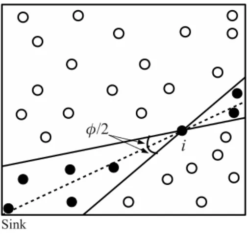
In this work, we consider that the data communication in a WSN is either from the sink to sensor nodes or vice-versa. Thus, the shortcuts to be added should be devised considering this communication pattern to optimize the data communication between sink and sensor nodes. In this section, we present a model in which all shortcuts are generated using an angulation directed to the sink.

(41)

H-sensors2

. The shortcuts are created considering the straight line y = mx+b that passes by the geographic position of each node and the geographic position of the sink node. This straight line is the bisectrix of an angle φ that deﬁnes an angle region directed to the sink node or opposite to it. Figure 3.2 shows the search space of a sensor nodei. Nodes that are in the direction of the data ﬂow between the sensor node

iand the sink node, represented as black nodes, can be chosen in the shortcut creation. The search space includes the direction opposite to the sink node since this direction will also help in the data communication process.

Figure 3.2. Directed angulation toward the sink model

To verify whether another node is inside its angulation region, a sensor node performs the following steps. Firstly, the node i calculates the straight line equation

y1 = m1x+b1 that passes by its geographic location and the sink node geographic

location. Secondly, the nodeicalculates the equation of the straight liney2=m2x+b2

that passes by its geographic location and the geographic location of node k, where

k �= i and node k is the node that we want to know whether it is in the angulation directed of nodei. The tangent of the angle formed by the two straight lines is given by the equation: tanθ = m1−m2

1+m₁m₂. Thus, the node i can determine if a given node is

inside the angleφdirected angulation making tanθ <tanφ₂.

Using these shortcuts, we create the small world model as follows. Consider a regular graph G(V, E). Given an edge e ∈ E | e = (vi, vj), where vi, vj ∈ V, it is

necessary to add an edgee�_{between nodes}_v

iandvk ∈ V in such a way thate�= (vi, vk),

where tanθ = mi−mk

1+mimk < tan

φ

2, vi, vk ∈ V and mi and mk are the angular coeﬃcients

of the straight line that passes through node i and the sink node and through node i

2

(42)

and nodek. The addition of this edge is done using the same probabilityp determined for each edge ofG. These steps are repeated for all edges ofG.

(a) p= 0.0001 (b) p= 0.001

(c)p= 0.01 (d) p= 0.1

Figure 3.3. Creation of shortcuts when the value of p changes in the TDASM

model (φ= 30◦₎

(43)

the next section, we present the values of the path length and the clustering coeﬃcient for diﬀerent values of the probabilityp.

3.3 On-line Model to Design HSNs

In a WSN, the random addition and the directed angulation toward the sink node models cannot be directly applied to the HSN creation due to two reasons. Firstly, in these models, to choose the endpoints of a shortcut, each node has to have the localization of all nodes in the network. In WSNs, due to the hardware and mainly energy restrictions, this assumption is infeasible because of the possibly large number of packets transmitted in the network. Secondly, in these models, a node chooses randomly another node to create a unicast link (shortcut) between them. The direct application of these models would lead to a planned deployment of H-sensors nodes, since they are endpoints of the shortcuts, which might be the case for an oﬀ-line model as discussed earlier. However, there are many WSN applications that assume a random deployment of sensor nodes, and, thus, need an “on-line” model. The random addition and the directed angulation toward the sink node are theoretical models to create networks with small world features, which we identify as TRAM (Theoretical Random Addition Model) and TDASM (Theoretical Directed Angulation toward the Sink node Model), respectively. These theoretical models can be executed before the deployment of the sensor nodes, i.e., they are oﬀ-line models.

When we consider the restrictions of the theoretical models to design an on-line solution, i.e., using a random deployment of sensor nodes, we have to adapt them to create a HSN. The on-line model is a way to implement the theoretical model in a distributed fashion for real applications and it was designed to preserve the small world features of the theoretical models. To create the on-line model, we evaluate the theoretical models and, based on their probability p of shortcut addition, we obtain the following parameters: (i) the number of endpoints (H-sensors); (ii) the number of shortcuts created per H-sensor; and (iii) the neighboring H-sensors that are the number of H-sensors inside the communication radius of a speciﬁc H-sensor for TRAM, or the number of H-sensors inside the directed angulation area for TDASM.

(44)

each sensor and the number of sensors inside the communication radius of each H-sensor (values obtained upon evaluating the theoretical models). The value ofp�_deﬁnes

the probability of creating a shortcut between two H-sensors. In this way, for both the On-line Random Addition Model (ORAM) and the On-line Directed Angulation toward the Sink node Model (ODASM), each deployed H-sensor in the network uses the probability p� _{for adding a shortcut between them. Using this scheme, for each}

value of probabilityp, we have the number of H-sensors created and, consequently, the value ofp� _{that represents the probability of shortcut addition between two H-sensors}

in the on-line models.

It is important to point out that, while the theoretical models require each node to know the position of all other sensors, in the on-line model, the H-sensors only need to know the geographic position of other H-sensors that are within their communica-tion range (neighboring H-sensors) and the Sink’s posicommunica-tion. This is due to the fact that each shortcut is created only between neighboring H-sensors. To ﬁnd the neighbor-ing H-sensors, all H-sensor nodes broadcast a hello message when the network starts operating.

If the network topology changes over time, due to the addition of new nodes, we can ﬁnd the neighboring H-sensors using well-known neighbor discovery protocols [Ra-manathan and Steenstrup, 1998; Borbash et al., 2007]. Another possibility to obtain the neighboring list is integrating diﬀerent layers of the protocol stack [Demirkol et al., 2006]. Several MAC protocols were proposed for wireless sensor networks [Ye et al., 2002; Enz et al., 2004; Ye et al., 2004] and most of them use a list of neighbors to syn-chronize the medium access. In this case, the routing protocol can be integrated with the MAC protocol and use the list of neighbors the MAC protocol has. In this case, the routing protocol has always an updated list of neighbors without additional cost. The next section presents the protocol design of the on-line version for both models.

3.4 Protocol Design of the On-line Model

Algorithm 1 describes the operation of the shortcut creation of the on-line directed angulation toward the sink node model. This algorithm is executed during the start-up time of each H-sensor. The variables used in the algorithm are:

• p�_{: probability of shortcut addition between a pair of neighboring H-sensors;}

• vi: geographic location of nodei;

(45)

• vk: geographic location of nodei’s neighbors (H-sensors);

• vsink: geographic location of sink node;

• mi: angular coeﬃcients of the straight line that passes through node i and the

sink node;

• mk: angular coeﬃcient of the straight line that passes through nodei and node

k;

• Lsi: shortcut list of node i.

The algorithm works as follows. At the beginning, node i sends a hello message containing its geographic location to all neighboring H-sensors and, after that, it re-ceives their locations (Lines 2 and 3). Initially, the list of shortcuts is empty (Line 4). In Line 5, node i calculates the angular coefficient of the straight line that passes through its geographic location and the sink ones. In Lines 6 to 13, the list of shortcuts for node iis created as follows. In Line 7, node i calculates the angular coefficient of the straight line that passes through its geographic location and the location of each neighboring H-sensor. In Line 8, nodeiverifies whether this angular coefficient is inside the angle region. If it is the case, the node chooses a probability at random and verifies if it is smaller thanp� _{when the node}_i_{sets its list of shortcuts (Lines 9 to 11). In Line}

14, nodeisends a message containing its list of shortcuts for all neighboring H-sensors that are endpoints of the created shortcut. When an H-sensor receives this message, it checks whether itself is inside the list. If this is the case, it updates its list of shortcuts. Otherwise, the H-sensor discards this message. In Line 15, the algorithm returns the list of shortcuts to be used for data communication among H-sensors. Algorithm 1 can be converted to the algorithm of ORAM removing Lines 5, 7, 8 and 12.

(46)

Algorithm 1 ODASM algorithm

1: procedure CreateShortcut(p�_{, v}

i) 2: broadcastHelloPacket(vi)

3: Li← receiveHelloPacket( )

4: Lsi← ∅

5: mi ←getAngularCoeﬃcient(vi, vsink) 6: for all vk ∈Li do

7: mk ← getAngularCoeﬃcient(vi, vk)

8: if mi−mk

1+mimk <tan

φ

2 then 9: if random( ) ≤p� _then

10: Lsi ←Lsi∪vk

11: end if

12: end if 13: end for 14: broadcast(Lsi) 15: return Lsi 16: end procedure

3.5 Complexity Analysis of the ODASM Algorithm

In this section, we will brieﬂy analyze the complexity of the ODASM algorithm in terms of communication requirements, processor resources, and time consumption:

• Communication complexity. In the ODASM algorithm, the H-sensor nodes start the shortcut creation by broadcasting their geographic location (Algorithm 1, Line 2). Each neighboring H-sensor that receives all broadcasts messages choses one or more neighboring H-sensors to create a shortcut between them. For this, the node sends a message to the other endpoints of the created shortcuts (Al-gorithm 1, Line 14). Thus, the communication complexity of our al(Al-gorithm is

O(H), where H is the number H-sensors deployed in the network, since each H-sensor sends two broadcast messages in the algorithm.

• Computational complexity. As mentioned before, the ODASM algorithm creates the directed search space by calculating the angular coeﬃcient between lines and by generating uniform random numbers. These procedures are quite simple and can be done using a small number of ﬂoat point operations.

(47)

proportional to the time to send two broadcast messages, which does not depend of the number of H-sensors or network nodes.

3.6 Simulation Results

3.6.1 Scenarios

In the simulation, we use a network with a total of 1000 nodes (L-sensors and H-sensors) randomly deployed in a sensor ﬁeld of 1000× 1000 m2_{. There is only one sink}

node located at the lower-left corner of the network. The communication radius of the L-sensors and H-sensors are 50 m and at most 500 m, respectively. For each generated topology, each L-sensor has an average of8 neighbors.

We evaluated diﬀerent angles φto deﬁne the search space (10, 20, 30, 40 and 50 degrees). However, when the angleφ is too small (10 or 20 degrees), the search space does not include enough nodes to create shortcuts. On the other side, when the angle

φ is too large (40 and 50 degrees), the search space is large enough to include nodes that are not directed to the sink node. Because of this behavior, the angle φequal to 30 degrees showed to be more appropriate, since this value is large enough to include a number of sensor nodes but not too large to include nodes that are not directed to the sink node. We used φequal to 30 degrees to evaluate our model.

All results correspond to the arithmetic average ofnsimulations, withndifferent network topologies, where n is defined according to the confidence interval desired in the simulation [Jain, 1991]. Let n= �₁₀₀_zs

ew

�2

, where s is the standard deviation, w is the average of the initial sample of10simulations3

, andz is the normal variate of the desired conﬁdence level. In all simulations, it was used a conﬁdence interval of 95%

(e= 0.05).

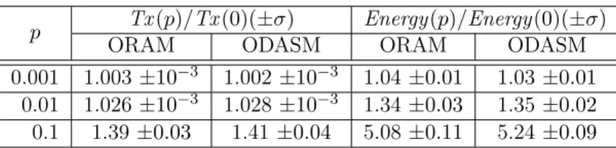
3.6.2 Small World Features Evaluation

In this section, we evaluate the average minimum path length4

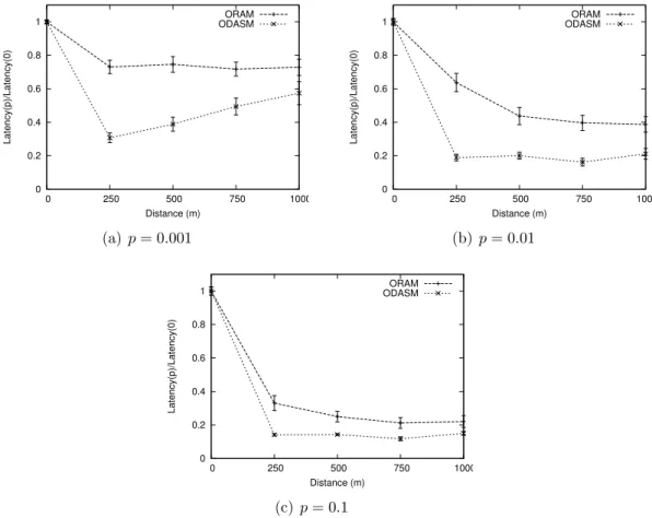
(L) and the clustering coefficient (C) of TRAM, TDASM, ORAM, and ODASM. In each generated topology, we evaluated the average minimum path length and the average clustering coefficient of the network. After n simulations, we obtain the average of these n results. The values C(0) and L(0) define the clustering coefficient and the average minimum path length of the WSN, respectively, with no shortcut addition (regular graph). The values

3

This value can be defined arbitrarily. The larger the initial sample, the smaller the value ofn.

4

(48)

C(p)andL(p)deﬁne the same parameters but for a probability p of shortcut addition probability. In all simulation results, it is calculated the ratio between C(p)/C(0) and

L(p)/L(0). This ratio clearly shows the inﬂuence of adding a fraction of shortcuts in the original regular graph.

Figure 3.4(a) illustrates the average minimum path length and the clustering coefficient of the theoretical random adding model when we change the value of the probability p. We observe that for small values of the probability (p < 0.001), the average minimum path length is reduced only 1.13times. This is due to the fact that the shortcuts are randomly generated and they do not contribute too much to reduce the average minimum path length between the sink and other nodes of the network. It is worth noting that forp <0.001, the clustering coefficient of the network is close to the one of a regular network. Then, for this value of probability, the network still presents characteristics of a regular graph. For values of p close to 0.01, this model generates a network with small world characteristics. Forp = 0.01, the average minimum path length is reduced 1.67 times and the clustering coefficient is close to the clustering coefficient of the regular graph. For values of probabilities close to 0.1, the average minimum path length is reduced 3.37 times and the clustering coefficient is reduced only 1.18 times, which lead to a network with small world characteristics. For values of p > 0.1, the average minimum path length does not reduce significantly. However, the clustering coefficient reduces fast, characterizing a random network.

0 0.2 0.4 0.6 0.8 1

0.0001 0.001 0.01 0.1 1 0 10 20 30 40 50 60 70 80 90 100

C(p)/C(0) and L(p)/L(0)

% of H−sensors

p C(r)/C(0) L(r)/L(0) H−sensors (a) TRAM 0 0.2 0.4 0.6 0.8 1

0.0001 0.001 0.01 0.1 1 0 10 20 30 40 50 60 70 80 90 100

C(p)/C(0) and L(p)/L(0)

% of H−sensors

p C(r)/C(0)

L(r)/L(0) H−sensors

(b) TDASM (φ= 30◦₎

Figure 3.4. Small world features of the theoretical models

Figure 3.4(b) shows the average minimum path length and the clustering coef-ﬁcient for TDASM. For p < 0.001, the average minimum path length is reduced 1.20

(49)

only 1.02 times. Again, the network exhibits small world characteristics. When the value of the probability is0.1, the average minimum path length is reduced4.06times and the clustering coeﬃcient only1.17times, and the network still keeps its small world characteristics. When the value of p is close to 1, the network presents random graph characteristics, once the average minimum path length and the clustering coeﬃcient are smaller than the one of a regular graph.

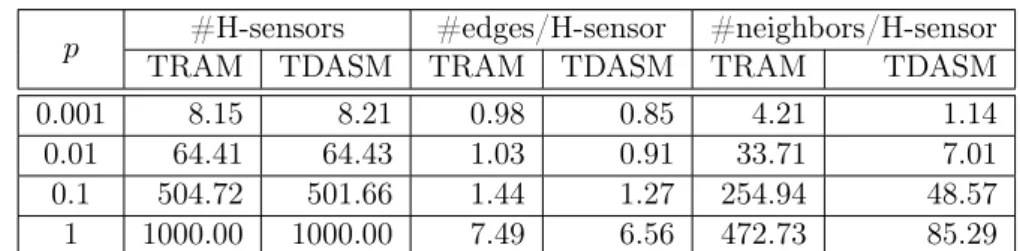
Table 3.1 shows the number of H-sensors deployed in the network, the number of edges created per H-sensor, and the number of neighboring H-sensors inside its communication radius. As discussed in Section 3.3, the on-line model receives the probability of adding a shortcut between a particular pair of H-sensors. In this case, when the probability of adding a shortcut between two nodes in the theoretical model isp, the probability of adding a shortcut in the on-line model isp� ₌ #edges/H−sensor

#neighbors/H−sensor.

As an example, forp = 0.01 in the theoretical model, the corresponding probabilities

p� _{in ORAM and ODASM are} _p� _{= 1}_.₀₃_/₃₃_._{71 = 0}_.₀₃ _and _p� _{= 0}_.₉₁_/₇_._{01 = 0}_.₁₂_,

respectively. ORAM has a smaller probability than ODASM because in the former an H-sensor has more neighbors than in the latter due to the angulation toward the sink. Using these values of probability, the number of shortcuts added per H-sensor in the on-line models is preserved, which allows us to maintain the desired average minimum path length (L) and clustering coeﬃcient (C), as depicted in Figure 3.5. Besides, we can have #edges/H-sensor<1 due to the fact that each edge is counted only once.

p #H-sensors #edges/H-sensor #neighbors/H-sensor

TRAM TDASM TRAM TDASM TRAM TDASM

0.001 8.15 8.21 0.98 0.85 4.21 1.14

0.01 64.41 64.43 1.03 0.91 33.71 7.01

0.1 504.72 501.66 1.44 1.27 254.94 48.57

1 1000.00 1000.00 7.49 6.56 472.73 85.29

Table 3.1. Number of added links for all models when we change the probability of shortcut addition

Figure 3.5 illustrates the average minimum path length and the clustering coef-ﬁcient of ORAM and ODASM. Recall that, for example, for p= 0.001, the real prob-ability of adding a shortcut between the H-sensors is p� ₌ #edges/H−sensor

#neighbors/H−sensor. Those