Evolutionary design of wireless sensor networks
based on complex networks
Andre S. Ruela
#1, Raquel S. Cabral
∗2, Andre L. L. Aquino
#3, Frederico G. Guimaraes
#4 #Department of Computer - Federal University of Ouro PretoOuro Preto, MG, Brazil 1[email protected]
∗
Department of Electrical Engineering - Federal University of Minas Gerais Belo Horizonte, MG, Brazil
Abstract—This work proposes a genetic algorithm for design-ing a wireless sensor network based on complex network theory. We develop an heuristic approach based on genetic algorithms for finding a network configuration such that its communication structure presents complex network characteristics, e.g. a small value for the average shortest path length and high cluster coefficient. The work begins with the mathematical model of the hub location problem, developed to determine the nodes which will be configured as hubs. This model was adopted within the genetic algorithm. The results reveal that our methodology allows the configuration of networks with more than a hundred nodes with complex network characteristics, thus reducing the energy consumption and the data transmission delay.
I. INTRODUCTION
Wireless Sensor Networks (WSNs) represent an emerging technology that allows the monitoring and control of physical and environmental variables and conditions, such as tempera-ture, sound, light, vibration, pressure, movement and pollution. A WSN consists of a great number of wireless autonomous devices, called sensor nodes, which work in a cooperative way to perform many different functions. These characteristics make the WSNs a promising technology in a wide range of application domains, for instance, biotechnology, industry, public health, and transportation ([1], [2]).
Despite its potential applicability, a WSN has several re-source restrictions, such as low computational power, reduced bandwidth, and limited energy source. Therefore, algorithms for WSNs need to be carefully designed. Thus, sending a large amount of data can be problematic, causing excessive delay in response time, invalidating the data. Moreover, a large traffic on the network can diminish its lifetime. Due to these restrictions, in some cases, it is necessary to adopt specific infrastructure designs to balance network requirements keeping its functionality.
Generally, the phenomenon monitored is reported through to sink considering a specific routing strategy. Examples of routing strategies are depicted in Figs. 1–3. A simple naive, but inefficient, way of propagating information through the network is flooding (Fig. 1). In this case, the information is flooded to all sensors until it reaches the sink node [3]. This
strategy causes unnecessary communication, consequently, a large energy consumption and a high response time to deliver the data.
Sink
Sensor Hub
Fig. 1. Flooding propagation.
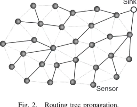
A common alternative to flooding is tree routing (Fig. 2), a simple and low-overhead routing protocol. Using a tree routing, each sensor is configured to send its data only to a specific sensor node, denoted father node. The choice of which node will be the father depends on the policy established by the application, in general, the shortest path policy is used [4]. The major drawback of tree routing is the increased hop counts as compared with more sophisticated path search protocols. However, there is a significant energy consumption because the link is kept, i.e., all non father nodes perceive the propagated data, this situation can be seen as light gray links in Fig. 2.
Sink
Sensor Hub
Fig. 2. Routing tree propagation.
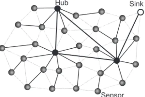
nodes working independently and together [5], some strategies based on tree routing might not be scalable. An alternative routing strategy based on complex network characteristics (Fig. 3), consists in setting some sensor nodes as hubs, these ones using a communication radius greater than used by normal nodes. Normal nodes propagate their data to a given hub using a normal link frequency, and the hubs propagate the data to the sink node using a special link frequency. In both cases it is used a multi-hop communication. The use of these hub nodes lead to important characteristics of complex networks: a small average shortest path length between all sensors and the sink; and a high cluster coefficient, see [6]. This complex network characteristics help us saving network resources, avoiding excessive communication, and reducing the time to data delivery.
Sink
Sensor Hub
Fig. 3. Complex network propagation.
In fact, the proposed approach gives rise to a complex network, which are networks with irregular, complex and dy-namic structure [7]. The theory of complex networks provides a mathematical framework for analyzing a number of real-world networks that otherwise could not be addressed with the available traditional models. The theory of complex networks can be useful in the study of WSNs, given some of its peculiar characteristics, such as the quantity, increase, and distribution of nodes in the network.
In this paper, we present a genetic algorithm for designing the logical topology for data propagation in a WSN. The goal here is to produce a logical topology that presents a high clustering coefficient and a small average shortest path length, which are two independent metrics from the complex network theory for quantifying structural features of the network. Exact methods are limited to small size networks, but for networks with hundreds or thousands of sensor nodes, the genetic algorithm becomes more interesting than the exact method from a practical point of view.
This paper is organized as follows. Section II shows the problem definition and its mathematical formulation. Sec-tion III, presents the soluSec-tion based on genetic algorithms. Section IV, discusses about the results obtained using the genetic algorithm. Finally, Section V concludes the paper.
II. PROBLEM DEFINITION
Consider a WSN as a regular graph G = (V, E), where
V represents the set of sensor nodes andE the set of edges,
representing the logical links between nodes. With this, the
problem addressed in this work can be stated as follows: Problem statement:Given a WSN, find the nodesv∈V that should be reconfigured as hubs, generating a new set of edges
E′
, such that a new networkG′
= (V, E′
) presents complex network characteristics.
For instance, the complex network characteristics
considered are only: the small shortest path length and a high cluster coefficient. However, the main hypothesis considered over the problem is:
Main hypothesis: By using a WSN with complex network characteristics it is possible to minimize the energy consumption and time in data delivery.
A. Problem Formulation
In this subsection, we present the mathematical formulation of the single allocation problem in sensor networks, which is an approach to the problem stated above.
Given a network with a set of nodes, the problem consists of finding the nodes that will be reconfigured as hub nodes and also the logical links that should be established in order
to minimize the total cost. LetN be the set of normal nodes
and H be the set of hub nodes, such that N ∪H = V and
N∩H =∅. The parameters of our mathematical model are:
φi communication demand, i.e., the total amount of data
that nodeimust send to the sink;
r basic communication radius;
dij distance between node iand nodej;
cij fixed communication cost per data unit from nodei
to nodej;
aj fixed installation cost of nodej as a hub node. It is
inversely proportional to the distance betweenj and
the sink, i.e., the higher the distance from j to the
sink, the lower the installation cost;
The decision variables of the mathematical model are:
• zi ∈ {0,1}: zi = 1 if node i is defined as hub, and
zi= 0, otherwise;
• qij ∈ {0,1}: qij = 1 if there is a logical link between
nodesiandj, andqij= 0, otherwise;
A nonlinear integer programming formulation of the prob-lem defined above is given by:
z∗
= arg minCI +CP (1)
subject to:
X
j∈V
qij= 1,∀i∈N (2)
X
j∈H
qij≤1,∀i∈H (3)
qij≤zj,∀i∈N,∀j ∈H (4) dijqij ≤r,∀i∈N,∀j∈H (5) dij≤2r,∀i∈H,∀j∈H (6)
where the installation cost CI is given by:
CI =
X
i∈V aizi,
and the propagation cost CP is given by:
CP =
X
i∈H
X
j∈N
φjcjiqji+φi
×
à X
k∈H
(cikqik+ck0) !
The objective function (1) gives the total cost for establish-ing the hub network. This total cost includes the installation
cost CI and the propagation cost CP. The first term in CP
represents the total amount of data that the hub i∈ H must
send to the sink, which is multiplied by the cost of sending
the data to the sink through hubk, wherekmay be equal toi
or may be a different hub. This gives two or three hops from any node in the sensor network to the sink.
The objective function (1) is subject to following con-straints:
(2) Guarantee that a node i ∈ N is connected to only
one hub.
(3) Guarantee that data from the hub i is either routed
through one hub or directly to the sink.
(4) Ensure that data from node i ∈ N is only routed
through a hub node.
(5) Ensure that the distance between the nodeiand a hub
node j is less than or equal to the communication
radius.
(6) Ensure that all hubs are within the range of all other
hubs, using twice the value of the communication radius.
(7) Restrict the values of the integer variableszi andqij
to assume either0 or1.
III. SOLUTION BASED ON GENETIC ALGORITHMS
In the context of combinatorial optimization problems, many metaheuristic techniques have emerged in the last thirty years [8], including Genetic Algorithms. In this paper, we present a GA to solve the problem presented in the previous section, the design of the logical routing structure in a WSN based on complex network theory.
A. Initial considerations
Our GA uses binary encoding to represent the network configuration, representing the nodes that are configured as
hubs. Each individual p(ti)in the populationPtis represented
by a binary vector ofV bits, whereV is the number of sensor
nodes,p(ti)[k] = 0indicates that the nodekis not configured
as a hub andp(ti)[k] = 1indicates that the nodekis configured
as a hub in the network structure encoded by this individual. Therefore, the encoding scheme represents a candidate routing structure.
We can define the following heuristics in order to eliminate
the decision variables qij in the GA:
• Given an individualp(ti)∈Pt, we obtain the set of nodes
inN and the set of hubs inH;
• As a general rule, every nodei∈N sends its data to the
hubj ∈H with the smallest costcij, usually the closest
one. In this way, we automatically have the corresponding
qij= 1;
• From each one of the hubs and the sink, the routing
is obtained using Dijkstra’s algorithm, respecting the maximum number of hops allowed.
With these simplifications, the variables qij are implicitly
calculated from the hub allocation provided by an individual
p(ti), thus simplifying the computation of the propagation cost
CP. The computation ofCI is simply given by the summation
of 1’s in p(ti). Moreover, constraints (2)-(4) can be neglected
in the model. We consider only the following constraints:
• The distance between a node i ∈ N and its associated
hub should be smaller than the communication radius r,
in other words, every node i ∈ N should have a hub
within its communication range.
• The distance from every hub to each other should be
smaller than twice the communication radius.
B. Simplified model
The considerations given above lead to the following model used for the GA:
minCI +CP (8)
subject to:
dij ≤r,∀i∈N, j= arg min
h {cih, h∈H} (9)
dij ≤2r,∀i, j∈H (10)
If one of these constraints is violated, then the value of the objective function is penalized giving the fitness function:
f(p(tk)) =CI+CP+w
X
i∈N
max [dij−r,0]2
+w X
u,v∈H
max [duv−2r,0]2,
(11)
withj= arg minh{cih, h∈H}.
C. Basic operators
The genetic algorithm implemented use tournament selec-tion for the reproducselec-tion, two-point crossover with probability
ρc= 0.8 and bit-flip mutation with probabilityρm= 0.1, see
([9], [10]) for further details.
The genetic algorithm for network configuration (Algo-rithm 1) considers:
• Line 2: Initialization operation.
• Line 3: The random initialization of a population withµ individuals that encode candidate configurations for the
problem. At each generationt, the population undergoes
the usual genetic operators, producing new candidate solutions for the problem.
• Lines 4–12: The loop that control the maximum number of interactions.
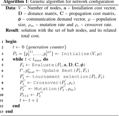
Algorithm 1: Genetic algorithm for network configuration
Data:V – Number of nodes,a – Installation cost vector,
D – distance matrix,C– propagation cost matrix,
φ φ
φ – communication demand vector,µ– population
size, ρm – mutation rate andρc – crossover rate.
Result: solution with the set of hub nodes, and its related total cost.
begin 1
t← 0{generation counter} 2
Pt={p
(1)
t , . . . , p
(µ)
t } ←Initialize(V, µ) 3
whilet < tmax do
4
Ft←Evaluate(Pt,a,D,C, φφφ) 5
t∗
, p∗
best←Update Best(Pt, Ft) 6
Pt′ ←tournament selection(Pt, Ft) 7
Pt′′←Crossover(P ′ t, ρc) 8
Pt′′′← Mutation(P ′′ t, ρm) 9
Pt+1←P
′′′ t 10
t←t+ 1 11
end 12
end 13
• Line 6: The best population is updated.
• Line 7: Individuals are selected for the reproduction stage using binary tournament selection, in which two
individuals are randomly selected from Pt, and compete
against each other. The one with the best fitness value
wins the tournament and goes toP′
t, thus having a chance
to reproduce. The best individuals are more likely to be selected for reproduction, but poor individuals also have some chance to be selected.
• Lines 8–9: A new population is formed from the selected individuals, using the crossover and mutation operators. • Lines 10–11: Incremental operations.
It should be emphasized that, although the genetic operators are random, the genetic algorithm is far from being a purely random search, because the selection operator has a determin-istic component that guides the searching process.
IV. COMPUTATIONAL RESULTS
The genetic algorithm searches for a WSN configuration that meets the complex network characteristics, i.e., a network having a small average path length between every node and the sink and a large clustering coefficient. Thus the data traffic is reduced, and consequently the energy consumption and the data delivery time are reduced. Initially, we present some general assumptions for the genetic algorithm evaluation:
• Simulations: The simulations were performed with the algorithm implemented in Java. The genetic algorithm
was executed considering a population of µ= 50
indi-viduals, for 500 generations. The number of necessary
simulations is given by [11],
rounds=³100z s p X
´2
,
where z is a constant of value 1.96, s is the standard
deviation found in the first simulations,X is the average
of the obtained values and p is the percentage of the
average that we want to get as deviation, which in this
case was5%.
We consider 30 rounds with random topologies, and for each topology we executed the genetic algorithm 33 times and the results are presented with symmetrical asymptotic confidence interval of 95%. The tests are executed in a machine Intel Quadcore 2.4GHz with 2GB RAM. • Network topology: The network density is kept constant,
the area is
A=π r2|S|/d,
wherer is the radio range, |S| is the number of sensor
nodes and d is network density (arbitrarily chosen with
the value31.4791).
The nodes started the execution with the same hardware configuration, at the end the hub nodes reconfigure the radio range based on the infrastructure solution. Thus, the final solution has a heterogeneous WSN.
• Resultant configuration: Considering G = (V, E) the
initial WSN graph and Gb = (V, Eb) the graph return
by the genetic algorithm. The resultant configuration,
used in a real network will be the graph G′ = (V, E′)
,
whereE′=E∪E
b. Thus, the cluster coefficient and the
average shortest path length are calculated considering those graphs. However, the number of installed hubs and the time to compute the results is showed.
Table I shows the results of the genetic algorithm with the
variation of the number of nodes (128,256,512,1024). The
evaluated parameters are: (i) number of installed hubs; (ii) execution time in seconds; (iii) cluster coefficient comparing
the initial regular graph G and the complex graph G′
; and (iii) average shortest path length comparing the initial regular
graphGand the complex graphG′
.
TABLE I
RESULTS CONSIDERING THE VARIATION OF THE NUMBER OF NODES(#).
# Hubs Time(s) Cluster coefficient Shortest path regular complex regular complex 128 11 44 0.689 0.691 2.550 2.659 256 24 353 0.657 0.650 3.381 2.729 512 68 4394 0.633 0.655 3.739 2.619 1024 252 49119 0.624 0.706 3.558 2.475
The results presented in Table I show that, with our genetic algorithm, it is possible to build a WSN with two specific complex network characteristics, the high cluster coefficient and the low average shortest path length. As we can see,
the cluster coefficient of the graph G′
is roughly the same
or slightly higher than that of the original regular graph G,
and the average shortest path length of the graph G′
for the
networks with sizes (256,512,1024) was reduced by 20%,
30%, and 31% respectively, when compared with the
required the installation of 11, 24, 68, and 252 hubs1 for the
networks with sizes(128,256,512,1024), respectively, which
gives a percentage of about 9%, 9%, 13%, and 25% of nodes installed as hubs.
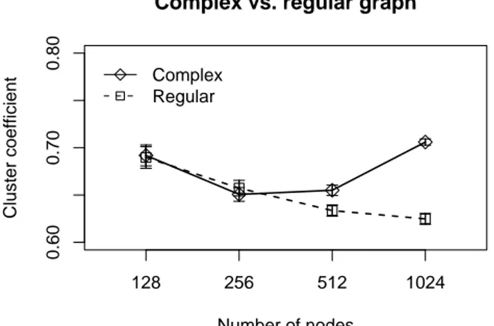
Complex vs. regular graph
Number of nodes
Cluster coefficient
Complex Regular
128 256 512 1024
0.60
0.70
0.80
Fig. 4. Cluster coefficient analysis.
Specifically, in Fig. 4 the cluster coefficient results are analyzed. In this case, when the number of nodes in the network is increased, the cluster coefficient of the resultant
graph G′
slightly increases with the number of nodes, while
that of the graph G always decreases. The installation of
hubs increases this coefficient because the normal nodes are connected only to hub nodes. Considering the WSN aspects, a high cluster coefficient reduces data delivery delays and unnec-essary energy consumption by concentrating the data sensing in a given hub node. Nevertheless, undesired interferences and link layer processing are avoided because the communication between hubs employs a different frequency range.
In Fig. 5 the average shortest path length results are pre-sented. In this case, when the number of nodes in the network increases, the average shortest path length slightly decreases
in the resultant graph G′
, while it increases in the graph G.
This occurs because the installation of hubs with a high radio range diminishes the shortest path in the network. Considering the WSN aspects, a low average shortest path length avoids, mainly, the data delivery delay. The drawback, in this case, is that when the radio range is modified more energy is consumed, but considering the global energy consumption this approach can actually save energy.
Finally, Fig. 6 shows the ratios of the cluster coefficient and the average shortest path length between the complex and
regular graphs. In this Figure,CCandSPrepresent the cluster
coefficient and the average shortest path length. In this case, when the number of nodes in the network is increased, the ratio of the average shortest path length is decreased while the ratio of the cluster coefficient remains close to one. This
1Nodes with differentiated radio range.
Complex vs. regular graph
Number of nodes
Average shortest path length
Complex Regular
128 256 512 1024
2.0
2.5
3.0
3.5
4.0
Fig. 5. Average shortest path length analysis.
Complex vs. regular graph
Number of nodes
SP(G’)/SP(G) and CC(G’)/CC(G)
SP(G’)/SP(G) CC(G’)/CC(G)
128 256 512 1024
0.6
1.0
1.4
1.8
Fig. 6. Ratios of the cluster coefficient and the average shortest path length between the complex and regular graphs.
behavior is evidence that the WSN obtained in this work can be a small world network [12], [13] or a scale free network [14], [15], but this assumption should be investigated more deeply.
V. CONCLUSION AND FUTURE RESEARCH DIRECTIONS This work presented a genetic algorithm for designing the logical topology for data propagation in a WSN. The goal was to produce a logical topology that presents a high clustering coefficient and a small average shortest path length, which are two independent metrics from the complex network theory for quantifying structural features of the network. For a network with 1024 nodes, the genetic algorithm was satisfactory, obtaining a network that satisfies the complex network characteristics.
characteris-tics, the high cluster coefficient and the low average shortest path length. This was highlighted in our results that showed that the cluster coefficient of the resultant graph is the same or slightly higher when compared to the original regular graph, and the average shortest path length of the resultant graph, in our specific scenario, was reduced by 20% or 30% when compared to the original regular graph.
This complex network strategy is important in WSNs be-cause a high cluster coefficient avoids the data delivery delay and unnecessary energy consumption by concentrating the data sensing in a given hub node. Interferences and link layer pro-cessing are avoided when different communication frequencies are used between hubs. The low average shortest path length avoids, mainly, the data delivery delay but on the other hand more local energy is consumed. This discussion shows the
truthfulness of the Main hypothesis presented in Section II.
Finally, features of more specific complex networks, e.g. small world or scale free networks, can be easily incorporated in the design of WSNs.
As future work we intend to implement an exact solution to show the efficiency of the genetic algorithm. Additionally, we intend to simulate the solutions provided by the genetic algorithm using available network simulators, in order to emphasize the advantages when using our solution design. Finally, we intend to implement a specific local search op-erator to improve the efficiency and robustness of the genetic algorithm implemented.
ACKNOWLEDGES
This work is partially supported by the Brazilian National Council for Scientific and Technological Development (CNPq) under the grant number 477292/2008-9.
REFERENCES
[1] I. F. Akyildiz, W. Su, Y. Sankarasubramaniam, and E. Cayirci, “A survey on sensor networks,”IEEE Communications Magazine, vol. 40, no. 8, pp. 102–114, August 2002.
[2] T. Arampatzis, J. Lygeros, and S. Manesis, “A survey of applications of wireless sensors and wireless sensor networks,” in13th IEEE Mediter-ranean Conference on Control and Automation (MED’05). Hawaii, USA: IEEE Computer Society, June 2005, pp. 719–724.
[3] M. Maroti, “Directed flood-routing framework for wireless sensor net-works,” in5th ACM/IFIP/USENIX International Conference on Mid-dleware (MidMid-dleware’04), vol. 78. Toronto, Ontario, Canada: ACM, October 2004, pp. 99–114.
[4] W. Qiu, E. Skafidas, and P. Hao, “Enhanced tree routing for wireless sensor networks,”Ad Hoc Networks, vol. 7, no. 3, pp. 638–650, May 2009.
[5] D. Estrin, L. Girod, G. Pottie, and M. Srivastava, “Instrumenting the world with wireless sensor networks,” in 26th IEEE International Conference on Acoustics, Speech, and Signal Processing (ICASSP’01), vol. 4. Salt Lake City, Utah, USA: IEEE Computer Society, June 2001, pp. 2033–2036.
[6] G. Sharma and R. Mazumdar, “Hybrid sensor networks: A small world,” in6th ACM International Symposium on Mobile Ad Hoc Networking and Computing (MobHoc’05). Urbana-Champaign, Illinois, USA: ACM, May 2005, pp. 366–377.
[7] S. Boccaletti, V. Latora, Y. Moreno, M. Chavez, and D.-U. Hwang, “Complex networks : Structure and dynamics,”Physics Reports, vol. 424, pp. 175–308, 2006.
[8] C. Blum and A. Roli, “Metaheuristics in combinatorial optimization: overview and conceptual comparison,”ACM Computing Surveys, vol. 35, no. 3, pp. 268–308, September 2003.
[9] D. E. Goldberg, Genetic Algorithms in Search, Optimization, and Machine Learning. Addison-Wesley Professional, 1989.
[10] M. Mitchell, An Introduction to Genetic Algorithms, ser. Complex Adaptive Systems. The MIT Press, 1998.
[11] R. K. Jain, The Art of Computer Systems Performance Analysis: Techniques for Experimental Design, Measurement, Simulation, and Modeling, C. P. Association, Ed. John Wiley & Sons, April 1991. [12] M. E. J. Newman and D. J. Watts, “Scaling and percolation in the
small-world network model,”Physical Review E, vol. 60, pp. 7332–742, 1999. [13] D. J. Watts and S. H. Strogatz, “Collective dynamics of small-world
networks,”Nature, vol. 393, pp. 440–442, 1998.
[14] A.-L. Barabsi and R. Albert, “Emergence of scaling in random net-works,”Science, vol. 286, pp. 509–512, 1999.