www.atmos-meas-tech.net/8/4979/2015/ doi:10.5194/amt-8-4979-2015
© Author(s) 2015. CC Attribution 3.0 License.
Evaluation of hierarchical agglomerative cluster analysis methods
for discrimination of primary biological aerosol
I. Crawford1, S. Ruske1, D. O. Topping1,2, and M. W. Gallagher1
1Centre for Atmospheric Science, SEAES, University of Manchester, Manchester, UK 2NCAS, National Centre for Atmospheric Science, University of Manchester, Manchester, UK
Correspondence to:I. Crawford ([email protected])
Received: 13 May 2015 – Published in Atmos. Meas. Tech. Discuss.: 16 July 2015
Revised: 6 November 2015 – Accepted: 10 November 2015 – Published: 27 November 2015
Abstract.In this paper we present improved methods for dis-criminating and quantifying primary biological aerosol par-ticles (PBAPs) by applying hierarchical agglomerative clus-ter analysis to multi-parameclus-ter ultraviolet-light-induced flu-orescence (UV-LIF) spectrometer data. The methods em-ployed in this study can be applied to data sets in excess of 1×10⁶points on a desktop computer, allowing for each fluorescent particle in a data set to be explicitly clustered. This reduces the potential for misattribution found in sub-sampling and comparative attribution methods used in previ-ous approaches, improving our capacity to discriminate and quantify PBAP meta-classes. We evaluate the performance of several hierarchical agglomerative cluster analysis linkages and data normalisation methods using laboratory samples of known particle types and an ambient data set.
Fluorescent and non-fluorescent polystyrene latex spheres were sampled with a Wideband Integrated Bioaerosol Spec-trometer (WIBS-4) where the optical size, asymmetry fac-tor and fluorescent measurements were used as inputs to the analysis package. It was found that the Ward linkage with z-score or range normalisation performed best, cor-rectly attributing 98 and 98.1 % of the data points respec-tively. The best-performing methods were applied to the BEACHON-RoMBAS (Bio–hydro–atmosphere interactions of Energy, Aerosols, Carbon, H2O, Organics and Nitrogen– Rocky Mountain Biogenic Aerosol Study) ambient data set, where it was found that thez-score and range normalisation methods yield similar results, with each method producing clusters representative of fungal spores and bacterial aerosol, consistent with previous results. Thez-score result was com-pared to clusters generated with previous approaches (WIBS AnalysiS Program, WASP) where we observe that the
sub-sampling and comparative attribution method employed by WASP results in the overestimation of the fungal spore con-centration by a factor of 1.5 and the underestimation of bac-terial aerosol concentration by a factor of 5. We suggest that this likely due to errors arising from misattribution due to poor centroid definition and failure to assign particles to a cluster as a result of the subsampling and comparative attri-bution method employed by WASP. The methods used here allow for the entire fluorescent population of particles to be analysed, yielding an explicit cluster attribution for each par-ticle and improving cluster centroid definition and our ca-pacity to discriminate and quantify PBAP meta-classes com-pared to previous approaches.
1 Introduction
Microorganisms influence climate through their physical and chemical interactions with the atmosphere. Recently there has been renewed interest in how primary biological aerosol particles (PBAPs) interact with and modify clouds. It has been shown that bacterial aerosol such asPseudomonas sy-ringaecan act as ice nuclei (IN) at relatively warm temper-atures (Möhler et al., 2007), which even in low concentra-tions can cause rapid cloud glaciation via the Hallet–Mossop process, leading to premature precipitation (Crawford et al., 2012).
fur-ther PBAP emission (Sands et al., 1982) – this is known as the bioprecipitation hypotheses, and potential links between long-term regional climatology and PBAP emissions have re-cently been suggested (Morris et al., 2014). One of the key drivers for new research into bioprecipitation is a need for more accurate quantification of cloud evolution and precipi-tation in weather and climate models given its potential im-pact.
Bioaerosols are now being included as important compo-nents in global climate models (Heald and Spracklen, 2009; Jacobson and Streets, 2009). Recently bioaerosol emission models were tested on European regional scales (Hummel et al., 2014) using real-time Wideband Integrated Bioaerosol Spectrometer (WIBS-4) data collected at rural and semi-rural sites in Germany and Finland (Toprak and Schnaiter, 2013; Schumacher et al., 2013). Validation of these models is re-liant on a very limited number of studies, and the authors highlight the difficulty of applying such models to e.g. urban environments and cite the general paucity of high-resolution atmospheric PBAP data to constrain model results. Providing such data is paramount to improving model predictions and accurately assessing the impact of PBAP emissions on envi-ronment and health. Retrieving such data is reliant upon the applicability of detection methods described in the following section.
The focus of this study is to evaluate hierarchical agglom-erative cluster analysis methods applied to WIBS ultraviolet-light-induced fluorescence (UV-LIF) data sets for the dis-crimination of primary biological aerosol. In this paper we describe the detection method and data preparation proce-dures before evaluating the performance of several common hierarchical agglomerative cluster analysis linkages and data normalisation methods using laboratory and ambient data sets.
Detection methods
The detection, classification and quantification of PBAPs remain a significant multidisciplinary technical challenge. Conventional techniques can be split into culturing and non-culturing techniques, both of which require the collection of particles onto a medium for offline analysis. Culturing tech-niques collect particles of interest onto a growth medium which is incubated for hours to days. The grown colonies are then counted microscopically, providing species identifi-cation but not quantifiidentifi-cation of their atmospheric concentra-tion, making the technique unsuitable for estimating PBAP emissions (Gabey, 2011). Non-culturing techniques collect particles onto filters or in a liquid suspension, which is more suitable for estimating atmospheric concentrations but is not typically used for classification (Douwes et al., 2003). The major limiting factors of non-culturing techniques are that they are labour intensive, require long sampling periods and suffer from impactor sampling artefacts (e.g. particle frag-mentation, obscuration), leading to erroneous enumeration.
This makes it difficult to study emissions at the process level as some PBAPs, such as fungal spores and bacteria, display large diurnal variations with significant short-term episodic emissions, which would require an impractical number of samples to capture reliably. PBAPs including bacteria can undergo substantial instantaneous spikes in emissions com-pared to their baseline state in response to rainfall (Crawford et al., 2014; Hummel et al., 2014). These rapid emissions are important not only to capture peak concentrations but also to derive emission factors accurately and understand the under-lying mechanisms.
UV-LIF spectrometers have become available which show early promise of classifying and quantifying bioaerosols by broad taxonomic class on a single-particle basis (Craw-ford et al., 2014; Gabey et al., 2013). This instrument is based on technology developed by the University of Hert-fordshire Centre for Atmospheric and Instrumentation Re-search (CAIR). A full technical description of the WIBS instrument is given later in this manuscript. UV-LIF spec-trometers work on the principle that PBAPs contain biofluo-rophores such as NAD(P)H, riboflavin, and tryptophan which auto-fluoresce when excited with UV radiation with the ex-citation, and detection bands of the WIBS are optimised to detect these common biofluorophores (Kaye et al., 2005). The single-particle, online nature of the technique yields far superior time resolution to the offline techniques discussed earlier, making it ideally suited to measuring PBAPs in a rapidly changing environment. The time resolution is limited by the counting statistics, with typically 1–5 min integration periods providing adequate sensitivity depending on ambi-ent concambi-entrations. This allows for better measuremambi-ents of PBAP fluxes, which would be difficult using traditional of-fline methods.
Whilst UV-LIF spectrometers offer many advantages over traditional methods, discriminating between different bioaerosol classes and possible, non-biological fluorescent interferents remains an ongoing area of research (Toprak and Schnaiter, 2013). At present, UV-LIF spectrometers lack a common absolute reference standard, making comparison of measurements made between instruments difficult. Further-more the lack of a calibration standard has impeded attempts to characterise PBAPs of interest which would greatly sim-plify classification by the utilisation of supervised learning techniques. In lieu of an absolute calibration method other techniques must be used to segregate particles by type when interpreting uncalibrated data sets.
2 WIBS UV-LIF instrumentation
to-tal as aerosol flow drawn through a 1.2 mm (inner diame-ter) tube to generate a single in-line aerosol beam intersect-ing a well-defined optical sensintersect-ing region. The remainder of the flow is filtered and used as a sheath flow to stabilise the aerosol beam and minimise possible detrainment contami-nation of the optical surfaces within the scattering cham-ber. Single particles passing through the sensing region in-tercept a 635 nm diode laser beam, and the elastically scat-tered forward and sideways intensity is measured. A lookup table based on a standard Mie scattering model (Kaye et al., 2005) is used to convert the forward-scatter / side-scatter in-tensity ratio to optical diameter based on the instrument’s re-sponse to NIST calibration polystyrene latex (PSL) spheres. The WIBS utilises a quadrant detector to measure the scat-tered intensity. The signal from each component quadrant is used to calculate an “average” optical diameter over the four scattering solid angles. In addition the standard devia-tion between the four signal intensities is used to provide a particle asymmetry factor (AF) as a proxy of particle mor-phology. AF is reported in arbitrary units (a.u.) and is based on measurements with calibration particles with different as-pect ratios; corn starch flour was used to represent irregu-lar particles, and ellipsoidal haematite particles were used as an analogue for rod-like bacterial particles as described in Kaye et al. (2007). AF ranges from 8 to 10 for nearly spherical particles and 20–100 for a rod- or fibre-like parti-cles. The detectable particle “average optical diameter” range for WIBS-4 is 0.5< Do<20 µm, with a 50 % detection at Dp50=0.8 µm (Gabey et al., 2011). The WIBS size range is optimised to sample most airborne bacteria and fungal spores, but only very small pollen. Following initial particle detection and sizing, two optically filtered Xenon flash-lamps are sequentially triggered, providing excitation wavelengths centred at 280±10 and 370±20 nm. The fluorescence emis-sion is collected by two spherical mirrors and split into two channels using a dichroic filter at 410 nm before being mea-sured by two photomultiplier tubes (PMTs).
Both PMTs record fluorescence during the 280 nm tation phase because no detection bands overlap the exci-tation band; however only the 410–650 nm PMT detector is active during the 370 nm excitation. In subsequent dis-cussions herein the three fluorescent channels will be re-ferred to as FL1 (fluorescence between 300 and 400 nm, following excitation at 280 nm), FL2 (fluorescence between 410 and 650 nm, following 280 nm excitation) and FL3 (flu-orescence between 410 and 650 nm, following excitation at 370 nm). The autofluorescence arising from the 280 nm exci-tation in biological material is influenced heavily by proteins and the bio-molecule tryptophan, whereas fluorescence from 370 nm excitation is influenced by riboflavin and co-enzyme NAD(P)H (Stanley et al., 2011; Benson et al., 1979; Billinton and Knight, 2001; Foot et al., 2008; Kaye et al., 2005; Li and Humphrey, 1991). However, fluorescence emission spectra are inherently broad, and interrogating complex microorgan-isms and micron-sized particles results in a complex mixture
of fluorescence emission peaks from many fluorophores that can be difficult to interpret unambiguously (Crawford et al., 2014; Pöhlker et al., 2012).
3 Hierarchical cluster methods
Hierarchical agglomerative cluster analysis (HCA) has been demonstrated to be a powerful tool to classify particles (Robinson et al., 2013; Crawford et al., 2014; Gabey et al., 2013); however, the available analysis toolkits are limited by heavy computational burdens, making the analysis of large data sets problematic. In HCA each data point is initially in its own single membered cluster. The clusters are sequen-tially combined into larger multi-membered clusters until all data points are in one large cluster at the end of the process. At each step through the process the two clusters which are separated by the shortest distance are combined where the inter-cluster distance is determined by the linkage algorithm. In this study we trialled several common linkages, which are now described:
– Single: the distance between two clusters is defined as the minimum distance between any single data point in the first cluster and any single point in the second clus-ter.
– Complete: the distance between two clusters is defined as the maximum distance between any single data point in the first cluster and any single point in the second cluster.
– Average(unweighted average distance): the distance be-tween two clusters is defined as the average distance between all data points in the first cluster and all data points in the second cluster. The weight of each cluster is proportional to the cluster size.
– Weighted(weighted average distance): similar to aver-age, but the weight of each cluster is identical irrespec-tive of size.
– Ward: this linkage is a special case where the clusters to be merged is determined by finding the pair of clus-ters which yield the minimum increase in total within-cluster variance after merging, rather than by minimum distance between clusters.
– Centroid: the distance between clusters is defined as the distance between the centres (mean vectors) of clusters. – Median: the distance between two clusters is iteratively defined as the distance between the cluster midpoints. Here the midpoint is defined as the point itself in a sin-gleton cluster or the average of the midpoints of the clusters to be merged.
3.1 WASP
The WIBS AnalysiS Program (WASP; Robinson et al., 2013) uses the average linkage clustering algorithm and is written in Igor Pro1. WASP performs HCA on a random subset of the data limited to a maximum of≈1×10⁴data points, with analysis taking around 4 h on a high-powered desktop com-puter2. The choice of the number of clusters to retain is man-ually selected by the inspection of several metrics, and the remaining data are attributed to the chosen clusters by com-parison to the cluster centroids using a distance-based simi-larity method as described in Robinson et al. (2013). The au-thors noted that this comparative method can lead to system-atic misattribution when less populous clusters form poorly defined centroids which do not reflect the true spread of the variables. They also noted that particles outside of a specified distance from a cluster centroid are left unclassified, poten-tially leading to an underprediction of cluster concentrations. 3.2 Fastcluster
In this manuscript we use open-source HCA methods which can analyse data sets in excess of 1×10⁶points on a desktop computer. Subsampling and comparative attribution are not required as each data point is explicitly clustered. We also test the feasibility of using an automated method for deter-mining the optimum number of clusters to retain.
In this study we have used the open-source Python pack-age fastcluster (Müllner, 2013), which features several com-mon linkages. Of the included linkages the Ward, centroid and median linkages do not require the distances between data points to be stored in memory, allowing for memory-saving modes to be used, greatly increasing the maximum number of data points that can be analysed from approx-imately 7×10⁴ to in excess of 1×10⁶ points using the test computer described earlier. In order to take advan-tage of the memory-saving algorithms, the Euclidean dis-tance metric must be used. The performance of the memory-saving linkages are assessed using laboratory-sampled par-ticles of known type and ambient data previously analysed with WASP. In a future publication we will assess computa-tional requirements in more detail, presenting results perti-nent to “big-data” analysis depending on the amount of data retrieved during any given campaign.
3.3 Overview of analysis procedure
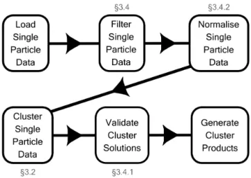
In this section we provide an overview of the procedure followed when applying hierarchical agglomerative cluster analysis to WIBS data (summarised in Fig. 1):
1. load and quality assure data; 1WaveMetrics Inc., OR, USA
23.4 GHz quad core, eight-thread processor, 16 GB RAM, 64 bit
OS.
Figure 1.Schematic of procedure followed to generate cluster prod-ucts from raw data. Relevant sections for each sub-procedure are labelled where appropriate.
2. filter data;
a. remove particlesDp<0.8 µm; b. remove non-fluorescent particles; c. remove saturating particles. 3. normalise data;
4. cluster data;
5. validate cluster solutions; 6. generate cluster products.
These procedures are now discussed. 3.4 Data preparation
Prior to analysis it is necessary to prepare the single-particle data to ensure that they are physically meaningful to prevent artefacts biasing the cluster solutions such that any poten-tial to effect the performance of any cluster analysis is min-imised.
The particle collection efficiency of the WIBS drops be-low 50 % at∼0.8 µm. We have chosen to integrate number concentrations of particles>0.8 µm rather than apply a cor-rection factor to the concentrations below this size.
a particle to be considered fluorescent it must exhibit a fluo-rescence greater than a threshold value, defined as the base-line fluorescence plus 3 SDs (standard deviations). The anal-ysis software subtracts this threshold value from measured fluorescence of each sample, with all values greater than 0 being considered significantly fluorescent compared to the instrument baseline. Fluorescence measurements below the threshold (i.e. less than 0 after threshold subtraction) are not considered physically meaningful and are clipped at 0. This simplifies the segregation between fluorescent (FL) and non-fluorescent (non-FL) particles.
Sufficiently fluorescent particles (such as pollens) will sat-urate the PMT, and as such it is not possible to accsat-urately measure their true fluorescence. Data from saturating par-ticles are not physically meaningful and are excluded from analysis.
3.4.1 Cluster validation indices
In order to remove the subjective nature of the method em-ployed by Robinson et al. (2013) to determine the optimum number of clusters to retain, we have chosen to use the Calinski–Harabasz criterion (CH), which is defined as being the ratio of the overall between-cluster variance to the overall within-cluster variance (Calinski and Harabasz, 1974). We calculate the CH index for the first 20 cluster solutions and select the solution with the highest CH value as being the optimal solution.
3.4.2 Data normalisation
In the Robinson et al. (2013) study the prepared data were z-score-normalised prior to analysis. This was performed to minimise the effect of the different ranges of scale of each parameter biasing the clustering; i.e. the fluorescent intensi-ties are of the scale 0–2092, size 0.8–20 and AF 0–100. We investigate the effect of normalisation on clustering perfor-mance using the following standard procedures:
1. No normalisation.
2. Subtract mean; divide by standard deviation (z-score). The mean value of the normalised distribution is 0, where the z-score value of a data point is the number of standard deviations from the mean. This can be posi-tive or negaposi-tive.
3. Standardise by range. Subtract minimum value; divide by the maximum value. Normalises data to new range of 0–1.
4. Divide by sum. Divide each of the variables by its sum. The sum of the normalised distribution is 1. Since our original data are positive, the normalised values will also be positive.
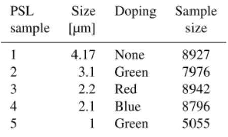
Table 1.Properties of the polystyrene latex spheres sampled.
PSL Size Doping Sample
sample [µm] size
1 4.17 None 8927
2 3.1 Green 7976
3 2.2 Red 8942
4 2.1 Blue 8796
5 1 Green 5055
5. Rank. Replace each data point by its rank. The data under this normalisation will be integers from 1 toN, whereNis the number of data points.
These are the procedures considered in Milligan and Cooper (1988) but excluding procedures which produce identical re-sults for the Euclidean metric. They concluded the range nor-malisation to be the best performing. We considered proce-dures proposed by Gnanadesikan et al. (2007) which consid-ered better-performing alternatives to the above procedures. However it seems unlikely that the procedures will scale in terms of performance for large data.
4 Data sets and data preparation
To assess the performance and suitability of the available clustering linkages, we first look at a laboratory data set of known particle types so that the cluster solutions can be com-pared to the known result. We then trial the best-performing methods on ambient data from the BEACHON-RoMBAS (Bio–hydro–atmosphere interactions of Energy, Aerosols, Carbon, H2O, Organics and Nitrogen–Rocky Mountain Bio-genic Aerosol Study) experiment, which has been studied previously using similar methods (Robinson et al., 2013; Crawford et al., 2014). These data sets are now described in detail.
4.1 Fluorescent polystyrene latex spheres
To test the applicability and performance of the memory-efficient hierarchical agglomerative clustering linkages avail-able in the Python package fastcluster, five different PSL spheres3were sampled using the WIBS-4. They were of dif-ferent sizes, and four of them had been doped with a fluo-rescent coating. The properties of the tested PSLs are sum-marised Table 1.
The three fluorescence measurements (FL1–3), size and asymmetry factor were chosen as inputs. The PSLs exhibit strong fluorescence, with some saturating the PMTs in multi-ple channels; as such we have chosen to keep saturating parti-cles in the analysis to maximise sample size. Non-fluorescent 3Manufactured by Polysciences Inc., PA, USA, and Duke
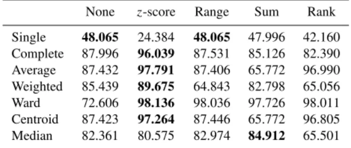
Table 2.Performance of the different linkages and normalisation procedures for the full data set in terms of the percentage of data points placed into the same cluster as the known clustering. In bold are the best-performing normalisations for each linkage.
None z-score Range Sum Rank
Single 48.065 24.384 48.065 47.996 42.160 Complete 87.996 96.039 87.531 85.126 82.390 Average 87.432 97.791 87.406 65.772 96.990 Weighted 85.439 89.675 64.843 82.798 65.056 Ward 72.606 98.136 98.036 97.726 98.011 Centroid 87.423 97.264 87.446 65.772 96.805 Median 82.361 80.575 82.974 84.912 65.501
particles and particles smaller than 0.8 µm have been ex-cluded from the analysis due to low collection efficiency. AF and size are typically log-normally distributed. In keeping with the analysis performed in Crawford et al. (2014) and Robinson et al. (2013) we convert these variables to log space prior to analysis. As memory saving is used, this limits anal-ysis to using only the Euclidean distance metric.
4.2 The regional BEACHON-RoMBAS experiment The WIBS was deployed at the the Manitou Experimen-tal Forest Observatory (MEFO), located 35 km northwest of Colorado Springs, Colorado, USA (Ortega et al., 2014; Kim et al., 2010), as part of the Rocky Mountain Biogenic Aerosol Study project (BEACHON-RoMBAS) during sum-mer 2011. Details of the experiment and sampling arrange-ment are given in Crawford et al. (2014). In the Crawford et al. (2014) study HCA was performed on a subset of the WIBS data (≈1×10⁴particles) using the average linkage, with the remaining particles attributed to a cluster by compar-ison to the cluster centroid. Details of the attribution method and the process of selecting the number of clusters to re-tain are provided in Robinson et al. (2013). This analysis yielded clusters which were behaviourally consistent with fungal spores and bacteria. We perform analysis of this data set using the methods described in this manuscript, which we compare to the Crawford et al. (2014) results.
5 Results
5.1 Fluorescent polystyrene latex spheres
The fastcluster package was run with the seven available linkages, each with the different normalisation procedures. Note that only the single, Ward, centroid and median link-age are available when the memory-efficient version of the fastcluster package is used.
Table 3.Performance of the Ward linkage for varying sample size.
Sample 500 1000 5000 10 000 20 000 size
z-score 79.330 85.696 94.746 97.543 97.132 Range 95.664 97.671 98.041 98.065 98.074
We use the CH index to identify the “optimal” number of clusters and attempt to construct a best match between the desired clusters and proposed clusters. Then, to evaluate the performance of the algorithm, we calculate the proportion of the data points placed into the same cluster for both the desired and proposed clustering. The results are given in Ta-ble 2.
For the full data set we can see that thez-score is the best-performing normalisation for all but the single and median linkages, where the performance is poorer across all normal-isations.
However in Table 3 we repeat the tests for varying sample size, where we see that as sample size decreases the range normalisation starts to outperform thez-score.
It appears that when using the full data set thez-score nor-malisation with either the Ward linkage or average linkage is the preferred option. When sampling, however, we see that range normalisation may be better.
An explanation for this behaviour could be that the range normalisation suffers with outliers which we are much more likely to encounter for large samples, so we would expect better performance for the smaller samples. Contrast this with thez-score where our measurement of the mean and the standard deviation is more accurate with large samples.
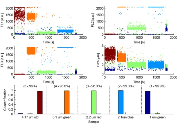
Figure 2.Top panel: average FL1–3 detector intensites (blue, green and brown bars, left axis), size (diamond, right axis) and asymmetry factor (cross, right axis) for the five PSL samples. Middle and bottom panels: the same as for the top panel but for the Ward linkage solution centroids using range (middle) andz-score (bottom) normalisation.
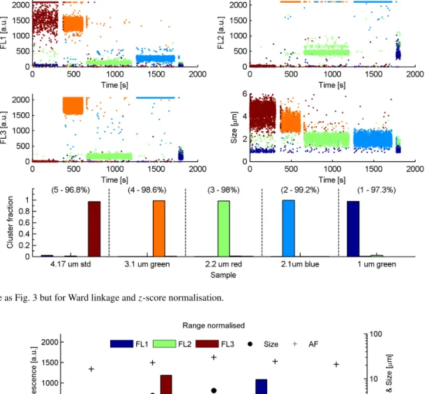
Figure 4.Same as Fig. 3 but for Ward linkage andz-score normalisation.
Figure 5.Same as Fig. 2 but for BEACHON-RoMBAS ambient data.
performed well, correctly attributing 97.3 % of the particles into five significant clusters.
5.2 BEACHON-RoMBAS
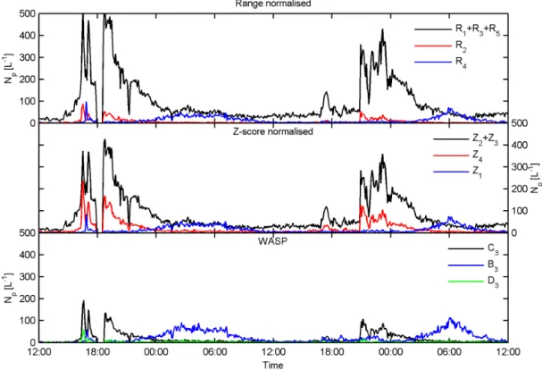
nor-Figure 6.Time series of BEACHON-RoMBAS cluster concentrations using Ward linkage with range (top panel) andz-score (middle panel) normalisation as compared to the solutions obtained using WASP (bottom panel) for the period 00:00 MST (Mountain Standard Time) on 26 July 2011 to 12:00 MST on 28 July 2011. Clusters with similar centroids have been combined. See text for details.
Figure 7.Size distribution of BEACHONz-score-normalised clus-ters produced using the Ward linkage for the period 00:00 to 06:00 MST 27 July 2011.
malisations and also the centroid linkage with z-score normalisation. The centroid linkage yielded a solution with only one significantly populated cluster, suggesting that it is inappropriate for analysing ambient data. Figure 5 shows the cluster centroids of each Ward normalisation where the range yields a five-cluster solution andz-score a 4-cluster solution. It can be seen that the solutions of each
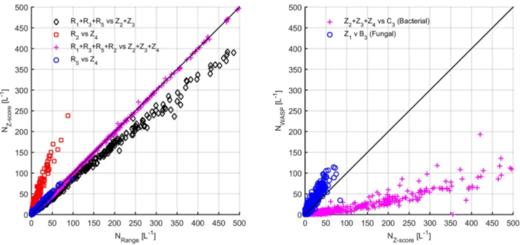
Figure 8.Left panel: comparison of Ward linkage cluster concentrations using range andz-score normalisation for BEACHON-RoMBAS. Right panel: comparison of Ward linkage cluster concentrations (z-score normalisation) to WASP cluster concentrations.
interpreting or assigning a bioaerosol meta-class to a cluster to avoid conflation of different particle types; e.g. emissions of some fungal spore species are positively correlated rain-fall, which could be conflated into the bacterial meta-class in this case. Supporting measurements are needed to determine which species are present so that possible conflations can be identified and caveated appropriately.
Figure 8 compares the concentrations of the similar clus-ters for each normalisation method. Comparison of R5 to Z4(left panel, blue circles, representative of fungal spores) shows each method to yield similar concentrations. Compar-ison of the bacterial cluster concentrations yields poor corre-lation between methods when comparing the traces in Fig. 6 (left panel, black diamonds and red squares); however when the concentration of all clusters representative of bacteria are combined (left panel, magenta crosses) the correlation is excellent (Nzscore=1.00×Nrange−1.42,R2=1). This sug-gests that the major difference between the two different nor-malisation methods is how particles of similar types are par-titioned between the clusters.
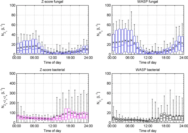
The right panel of Fig. 8 compares the z-score concen-trations to those obtained using WASP. It can be seen that the WASP fungal concentration is overestimated by a fac-tor of approximately 1.5 compared to thez-score result (Z4 andB3, blue circles). The WASP bacterial concentration is underestimated by approximately a factor of 5 compared to the z-score result. Figure 9 shows the hourly average diur-nal cycles of the fungal (top panels) and bacterial (bottom panels) cluster concentrations for thez-score result (left pan-els) and WASP (right panpan-els) over the period 27 July 2011– 7 August 2011. Each method displays a similar trend, with the fungal clusters exhibiting a minimum during the day ow-ing to the diurnal response of fungal spores to relative hu-midity and the bacterial clusters responding to the frequent afternoon rain storms (Crawford et al., 2014). Again it can be seen that WASP overestimates the fungal concentration by approximately a factor of 1.5–2 and underestimates the
bacterial concentration by a factor of 5–6 compared to the z-score result. The most likely explanation for the observed discrepancies between the WASP andz-score concentrations is the introduction of artefacts caused by the subsampling and comparative attribution methods used in WASP. In the fun-gal spore case, misattribution due to a poorly defined cen-troid can lead to an overestimation when compared to the new method as observed here. WASP yields only one cluster representative of bacteria, while thez-score method yields three and the range method four. This results in WASP fail-ing to attribute data points potentially representative of bac-teria to its single bacbac-terial cluster, leading to the observed underestimation when compared to the new method. WASP does not return diagnostic information about the cluster attri-bution; however, the sum of the concentration of WASP clus-tersB3,C3andD3only accounts for approximately 24 % of the fluorescent aerosol concentration, suggesting that many particles are left unattributed by WASP.
6 Conclusions
Figure 9.Top panels: hourly average diurnal cycle of fungal cluster concentration forz-score normalisation (left panels) and WASP (right panels) over the period 27 July 2011–7 August 2011. Bottom panels: same as for top panels but for the bacterial clusters. Whiskers denote 5th and 95th percentiles. Mean value indicated by x marker. Note change in scale for bacterial panels.
results for the same data set (Robinson et al., 2013; Crawford et al., 2014), where it was found that WASP overestimated the fungal spore concentration by a factor of 1.5 and under-estimated the bacterial aerosol concentration by a factor of 5 compared to the methods trialled here. This is likely due to errors arising from misattribution due to poor centroid def-inition and failure to assign particles to a cluster as a result of the subsampling and comparative attribution method em-ployed by WASP. The methods used here allow for the entire fluorescent population of particles to be analysed, yielding an explicit cluster attribution for each particle. This improves cluster centroid definition (e.g. allowing for several bacterial clusters compared to just one in WASP) and removes the po-tential for underestimation by failing to attribute a particle to a cluster.
In this paper we have demonstrated that WIBS single-particle UV-LIF spectrometer data can be successfully segre-gated using the Ward hierarchical agglomerative cluster anal-ysis linkage withz-score and range data normalisation. The explicit clustering method employed in this study can be ap-plied to large data sets, removing potential clustering aret-facts associated with the subsampling and attribution method used in previous approaches, improving our capacity to dis-criminate and quantify PBAP meta-classes. These improved techniques will be of importance for interpreting data from
future multi-parameter UV-LIF instruments with improved fluorescence resolution and for extending the measurement technique to real-time quantification for ambient monitoring networks.
The Supplement related to this article is available online at doi:10.5194/amt-8-4979-2015-supplement.
Acknowledgements. The authors wish to express our gratitude to R. Sarda Esteve (CEA) and J. A. Huffman (University of Denver) for use of their fluorescent calibration particles as part of the BIODETECT experiment, without which the fundamentals of this work could not have been performed. We would also like to acknowledge USFS and NCAR for providing invaluable logistical support and access to the Manitou Experimental Forest field site. We also acknowledge P. Kaye and W. R. Stanley (University of Hertfordshire) for their continued support. This work was funded by the Natural Environment Research Council INUPIAQ programme, grant number NE/K006002/1.
References
Benson, R., Meyer, R., Zaruba, M., and KcKhann, G.: NoCellular autofluorescence – is it due to flavins?, J. Histochem. Cytochem., 27, 44–48, 1979.
Billinton, N. and Knight, A. W.: Seeing the wood through the trees: a review of techniques for distinguishing green fluorescent pro-tein from endogenous autofluorescence, Anal. Biochem., 291, 175–97, doi:10.1006/abio.2000.5006, 2001.
Calinski, T. and Harabasz, J.: A dendrite method for cluster analysis, Commun. Stat.-Theor. M., 3, 1–27, doi:10.1080/03610927408827101, 1974.
Crawford, I., Bower, K. N., Choularton, T. W., Dearden, C., Crosier, J., Westbrook, C., Capes, G., Coe, H., Connolly, P. J., Dorsey, J. R., Gallagher, M. W., Williams, P., Trembath, J., Cui, Z., and Blyth, A.: Ice formation and development in aged, wintertime cumulus over the UK: observations and modelling, Atmos. Chem. Phys., 12, 4963–4985, doi:10.5194/acp-12-4963-2012, 2012.
Crawford, I., Robinson, N. H., Flynn, M. J., Foot, V. E., Gal-lagher, M. W., Huffman, J. A., Stanley, W. R., and Kaye, P. H.: Characterisation of bioaerosol emissions from a Colorado pine forest: results from the BEACHON-RoMBAS experiment, At-mos. Chem. Phys., 14, 8559–8578, doi:10.5194/acp-14-8559-2014, 2014.
Douwes, J., Thorne, P., Pearce, N., and Heederik, D.: Bioaerosol Health Effects and Exposure Assessment: Progress and Prospects, Ann. Occup. Hyg., 47, 187–200, doi:10.1093/annhyg/meg032, 2003.
Foot, V. E., Kaye, P. H., Stanley, W. R., Barrington, S. J., Gal-lagher, M., and Gabey, A.: Low-cost real-time multiparameter bio-aerosol sensors, in: Optically Based Biological and Chemical Detection for Defence, 71160I–71160I-12, 15 September 2008, Cardiff, Wales, UK, doi:10.1117/12.800226, 2008.
Gabey, A. M.: Laboratory and field characterisation of fluorescent and primary biological aerosol particles, PhD thesis, University of Manchester, Manchester, UK, 2011.
Gabey, A. M., Stanley, W. R., Gallagher, M. W., and Kaye, P. H.: The fluorescence properties of aerosol larger than 0.8 µm in ur-ban and tropical rainforest locations, Atmos. Chem. Phys., 11, 5491–5504, doi:10.5194/acp-11-5491-2011, 2011.
Gabey, A. M., Vaitilingom, M., Freney, E., Boulon, J., Selle-gri, K., Gallagher, M. W., Crawford, I. P., Robinson, N. H., Stanley, W. R., and Kaye, P. H.: Observations of fluorescent and biological aerosol at a high-altitude site in central France, Atmos. Chem. Phys., 13, 7415–7428, doi:10.5194/acp-13-7415-2013, 2013.
Gnanadesikan, R., Kettenring, J., and Maloor, S.: Better alter-natives to current methods of scaling and weighting data for cluster analysis, J. Stat. Plan. Infer., 137, 3483–3496, doi:10.1016/j.jspi.2007.03.026, 2007.
Heald, C. L. and Spracklen, D. V.: Atmospheric budget of primary biological aerosol particles from fungal spores, Geophys. Res. Lett., 36, L09806, doi:10.1029/2009GL037493, 2009.
Hummel, M., Hoose, C., Gallagher, M., Healy, D. A., Huff-man, J. A., O’Connor, D., Pöschl, U., Pöhlker, C., Robin-son, N. H., Schnaiter, M., Sodeau, J. R., Stengel, M., Toprak, E., and Vogel, H.: Regional-scale simulations of fungal spore aerosols using an emission parameterization adapted to local measurements of fluorescent biological aerosol particles, Atmos.
Chem. Phys., 15, 6127–6146, doi:10.5194/acp-15-6127-2015, 2015.
Jacobson, M. Z. and Streets, D. G.: Influence of future anthro-pogenic emissions on climate, natural emissions, and air qual-ity, J. Geophys. Res., 114, D08118, doi:10.1029/2008JD011476, 2009.
Kaye, P. H., Stanley, W. R., Hirst, E., Foot, E. V., Bax-ter, K. L., and Barrington, S. J.: Single particle multichan-nel bio-aerosol fluorescence sensor, Opt. Express, 13, 3583, doi:10.1364/OPEX.13.003583, 2005.
Kaye, P. H., Aptowicz, K., Chang, R. K., Foot, V., and Videen, G.: Angularly Resolved Elastic Scattering from Airborne Particles, Opt. Biol. Part., 238, 31–61, 2007.
Kim, S., Karl, T., Guenther, A., Tyndall, G., Orlando, J., Harley, P., Rasmussen, R., and Apel, E.: Emissions and ambient distribu-tions of Biogenic Volatile Organic Compounds (BVOC) in a pon-derosa pine ecosystem: interpretation of PTR-MS mass spectra, Atmos. Chem. Phys., 10, 1759–1771, doi:10.5194/acp-10-1759-2010, 2010.
Li, J. K. and Humphrey, A. E.: Use of fluorometry for monitoring and control of a bioreactor, Biotechnol. Bioeng., 37, 1043–1049 doi:10.1002/bit.260371109, 1991.
Milligan, G. W. and Cooper, M. C.: A study of standardiza-tion of variables in cluster analysis, J. Classif., 5, 181–204, doi:10.1007/BF01897163, 1988.
Möhler, O., DeMott, P. J., Vali, G., and Levin, Z.: Microbiology and atmospheric processes: the role of biological particles in cloud physics, Biogeosciences, 4, 1059–1071, doi:10.5194/bg-4-1059-2007, 2007.
Morris, C. E., Conen, F., Alex Huffman, J., Phillips, V., Pöschl, U., and Sands, D. C.: Bioprecipitation: a feedback cycle linking earth history, ecosystem dynamics and land use through biological ice nucleators in the atmosphere, Global Change Biol., 20, 341–351, doi:10.1111/gcb.12447, 2014.
Müllner, D.: fastcluster: fast hierarchical, agglomerative clus-tering routines for R and Python, J. Stat. Softw., 9, 1–18, doi:10.18637/jss.v053.i09, 2013.
Ortega, J., Turnipseed, A., Guenther, A. B., Karl, T. G., Day, D. A., Gochis, D., Huffman, J. A., Prenni, A. J., Levin, E. J. T., Krei-denweis, S. M., DeMott, P. J., Tobo, Y., Patton, E. G., Hodzic, A., Cui, Y. Y., Harley, P. C., Hornbrook, R. S., Apel, E. C., Mon-son, R. K., Eller, A. S. D., Greenberg, J. P., Barth, M. C., Campuzano-Jost, P., Palm, B. B., Jimenez, J. L., Aiken, A. C., Dubey, M. K., Geron, C., Offenberg, J., Ryan, M. G., Forn-walt, P. J., Pryor, S. C., Keutsch, F. N., DiGangi, J. P., Chan, A. W. H., Goldstein, A. H., Wolfe, G. M., Kim, S., Kaser, L., Schnitzhofer, R., Hansel, A., Cantrell, C. A., Mauldin, R. L., and Smith, J. N.: Overview of the Manitou Ex-perimental Forest Observatory: site description and selected sci-ence results from 2008 to 2013, Atmos. Chem. Phys., 14, 6345– 6367, doi:10.5194/acp-14-6345-2014, 2014.
Robinson, N. H., Allan, J. D., Huffman, J. A., Kaye, P. H., Foot, V. E., and Gallagher, M.: Cluster analysis of WIBS single-particle bioaerosol data, Atmos. Meas. Tech., 6, 337–347, doi:10.5194/amt-6-337-2013, 2013.
Sands, D., Langhans, V., Scharen, A., and de Smet,: The association between bacteria and rain and possible resultant meteorological implications, J. Hungar. Meteorol. Serv., 86, 148–152, 1982. Schumacher, C. J., Pöhlker, C., Aalto, P., Hiltunen, V., Petäjä, T.,
Kulmala, M., Pöschl, U., and Huffman, J. A.: Seasonal cycles of fluorescent biological aerosol particles in boreal and semi-arid forests of Finland and Colorado, Atmos. Chem. Phys., 13, 11987–12001, doi:10.5194/acp-13-11987-2013, 2013.
Stanley, W. R., Kaye, P. H., Foot, V. E., Barrington, S. J., Gal-lagher, M., and Gabey, A.: Continuous bioaerosol monitoring in a tropical environment using a UV fluorescence particle spectrom-eter, Atmos. Sci. Lett., 12, 195–199, doi:10.1002/asl.310, 2011. Toprak, E. and Schnaiter, M.: Fluorescent biological aerosol