Superfluid Bose-Fermi mixture from weak coupling to unitarity

Superfluid Bose-Fermi mixture from weak coupling to unitarity

S. K. Adhikari1,

*

and Luca Salasnich2,† 1

Instituto de Física Teórica, UNESP—São Paulo State University, 01405-900 São Paulo, SP, Brazil 2

CNR-INFM and CNISM, Unit of Padua, Department of Physics “Galileo Galilei,” University of Padua, 35122 Padua, Italy 共Received 23 August 2008; published 30 October 2008兲

We investigate the zero-temperature properties of a superfluid Bose-Fermi mixture by introducing a set of coupled Galilei-invariant nonlinear Schrödinger equations valid from weak coupling to unitarity. The Bose dynamics is described by a Gross-Pitaevskii-type equation including beyond-mean-field corrections possessing the correct weak-coupling and unitarity limits. The dynamics of the two-component Fermi superfluid is de-scribed by a density-functional equation including beyond-mean-field terms with correct weak-coupling and unitarity limits. The present set of equations is equivalent to the equations of generalized superfluid hydrody-namics, which take into account also surface effects. The equations describe the mixture properly as the Bose-Bose repulsive共positive兲and Fermi-Fermi attractive共negative兲scattering lengths are varied from zero to infinity in the presence of a Bose-Fermi interaction. The present model is tested numerically as the Bose-Bose and Fermi-Fermi scattering lengths are varied over wide ranges covering the weak-coupling to unitarity transition.

DOI:10.1103/PhysRevA.78.043616 PACS number共s兲: 03.75.Ss, 03.75.Hh

I. INTRODUCTION

The macroscopic quantum phenomenon of superfluidity has been clearly demonstrated in recent experiments with ultracold and dilute gases made of alkali-metal atoms 关1,2兴. Both bosonic and fermionic ultracold and dilute superfluids can be accurately described by the zero-temperature hydro-dynamical equations of superfluids关1–5兴.

Trapped Bose-Fermi mixtures, with Fermi atoms in a single hyperfine state共normal Fermi gas兲, were investigated by various authors both theoretically关6–14兴and experimen-tally关15–17兴. Recently, there was a study of a dilute mixture of superfluid bosons and fermions across a Feshbach reso-nance of the Fermi-Fermi scattering lengthaf, obtaining the phase diagram of the mixture in a box 关18兴. In the strict one-dimensional case, we found that the superfluid Bose-Fermi mixture exhibits phase separation and solitons by changing the Bose-Fermi interaction关19,20兴.

In the present paper we analyze in detail a three-dimensional 共3D兲superfluid Bose-Fermi mixture under har-monic trapping confinement when the Bose-Bose repulsive 共positive兲 and Fermi-Fermi attractive 共negative兲 scattering lengths are varied from very small 共weak coupling兲to infi-nitely large 共strong coupling兲values. The variation of these scattering lengths from weak to strong coupling is achieved in laboratory 关21兴 by varying a background magnetic field near a Feshbach resonance.

In the first part of the paper we derive Galilei-invariant nonlinear Schrödinger equations for superfluid Bose and Fermi dynamics, valid from weak-coupling to unitarity in each case, which are equivalent to the hydrodynamical equa-tions. For bosons the equation is a generalized关22–24兴 zero-temperature Gross-Pitaevskii 共GP兲 equation 关25兴 including beyond-mean-field corrections to incorporate correctly the

effect of bosonic interaction for large and positive共repulsive兲 scattering lengths a_b. In the ordinary GP equation the non-linear term is non-linearly proportional to ab and hence highly overestimates the effect of bosonic interaction for large posi-tive values of ab. In fact there is a saturation of bosonic interaction in the so-called unitarityab→+⬁limit, properly taken care of in the present generalized GP equations. For superfluid fermions the present formulation is based on the density-functional 共DF兲 theory 关26,27兴 for fermion pairs 关23,28–31兴 including beyond-mean-field corrections to in-corporate properly the effect of fermionic attraction between spin-up and -down fermions especially for large negative共 at-tractive兲values of Fermi-Fermi scattering lengtha_f. The DF theory, in different forms, has already been applied to the problem of ultracold fermions 关32,33兴. The usual DF equa-tion is valid for the weak-coupling Bardeen-Cooper-Schrieffer共BCS兲limit:a_f→−0. The present generalized DF equation correctly accounts for the dynamics as the Fermi-Fermi attraction is varied from the weak-coupling BCS limit to unitarity:af→−⬁. In the unitarity limit there is a satura-tion of the effect of fermion interacsatura-tion, properly taken care of in the present set of equations, which seems to be appro-priate to study the crossover 关34兴 from the weak-coupling BCS limit to the molecular Bose limit.

In the second part of the paper, by including the interac-tion between a boson and fermion pair, we obtain a set of coupled equations for superfluid Bose-Fermi dynamics in the presence of a Bose-Fermi interaction. The model correctly describes the dynamics as the Bose-Bose repulsion and Fermi-Fermi attraction are varied from weak coupling to uni-tarity. This model is tested numerically as the different scat-tering lengths are varied over wide ranges covering the weak-coupling to unitarity transition for a superfluid Bose-Fermi mixture.

In Sec. II we present the hydrodynamical equations for bosons and fermions and present the appropriate bulk chemi-cal potentials valid in the weak-coupling limit as well as possessing the saturation in the strong-coupling unitarity limit consistent with the constraints of quantum mechanics. *adhikari@ift.unesp.br; URL www.ift.unesp.br/users/adhikari

In Sec. III we derive mean-field equations for bosons and fermions consistent with the hydrodynamical equations for a large number of atoms. Next we derive the present model for interacting Bose-Fermi superfluid introducing a contact inter-action between bosons and fermions. In Sec. IV we perform numerical calculations for densities and chemical potentials of a trapped Bose-Fermi superfluid mixture to show the ad-vantage of the present model. Finally, in Sec. V we present a brief summary and conclusion.

II. SUPERFLUID HYDRODYNAMICS FOR BOSONS AND FERMIONS

At zero temperature, for a large number of atoms, statical and dynamical collective properties of bosonic and fermionic superfluids are expected to be properly described by the hy-drodynamical equations of superfluids关1,2兴. For bosons the hydrodynamical equations are given by关1,3兴

⳵

⳵_tnb+⵱·共nbvb兲= 0, 共1兲

mb ⳵

⳵_tvb+⵱

冉

1 2mbvb

2

+Ub+␮b共nb,ab兲

冊

= 0, 共2兲 whereU_b共r兲is the external potential acting on bosons,m_bis the mass of a bosonic atom, nb共r,t兲 is the local density of bosons, andvb共r,t兲is the local superfluid velocity关1–3兴. The total number of bosons is given by

Nb=

冕

nb共r,t兲d3r, 共3兲 and the nonlinear term␮b共nb,ab兲is the bulk chemical poten-tial of the bosonic system with ab the Bose-Bose scattering length. Equation 共1兲 is the equation of continuity of hydro-dynamic flow, while Eq. 共2兲 is the equation of conservation of the linear momentum. Equation共2兲establishes the irrota-tional nature of the superfluid motion: ⵜ_{⫻vb= 0, meaning} that the velocityvbcan be written as the gradient of a scalar field. Equations 共1兲 and 共2兲 differ from the corresponding equations holding in the collisional regime of a nonsuper-fluid system because of the irrotationality constraint.

For superfluid fermions, the fundamental entity governing the superfluid flow is the Cooper pair. In the case of a two-component共spin up and down兲superfluid Fermi system one can introduce the local density of pairs np共r,t兲=nf共r,t兲/2, wherenf共r,t兲 is the total local density of fermions. The hy-drodynamical equations of a fermionic superfluid 关2–5兴 can be written as

⳵

⳵tnp+⵱·共npvp兲= 0, 共4兲

mp ⳵

⳵_tvp+⵱

冉

1 2mpvp

2

+Up+␮p共np,af兲

冊

= 0, 共5兲 where the nonlinear term␮p共np,af兲is the bulk chemical po-tential of pairs with af the attractive Fermi-Fermi scattering length. Herempis the mass of a pair, that is twice the mass

mf of a single fermion, i.e.; mp= 2mf. In addition, the trap potential Up共r兲 is twice the trap potentialUf共r兲 acting on a single fermion, i.e., Up共r兲= 2Uf共r兲. Note that the chemical potential ␮_p共n_p,a_f兲 is twice the total chemical potential

␮f共nf,af兲 of the Fermi system, i.e.,␮p共np,af兲= 2␮f共2np,af兲. The total numberNf of fermions is

Nf= 2Np= 2

冕

np共r兲d3r=

冕

nf共r兲d3r, 共6兲 whereNp is the number of pairs.

It is important to stress that Eqs.共1兲and共2兲are formally similar to Eqs. 共4兲 and 共5兲, but the quantities involved are strongly different. In particular, the bulk chemical potential of bosons is completely different from the bulk chemical potential of Fermi pairs关1,2,35兴.

In the full crossover from the small-gas-parameter regime to the large-gas-parameter regime we use the following ex-pression for the bulk chemical potential of the Bose super-fluid 关22兴:

␮b共nb,ab兲= ប2 mb

n_b2/3f共n_b1/3ab兲, 共7兲 where

f共x兲= 4␲ x+␣x

5/2

1 +␥x3/2+␤x5/2. 共8兲 In the small-gas-parameter共x→0兲regime, Eq.共8兲becomes f共x兲= 4␲关x+共␣−␥兲x5/2+ ¯兴, 共9兲 which is the analytical result for bulk chemical potential found by Lee, Yang, and Huang 关36,37兴 in this limit, pro-vided that共␣−␥兲= 32/共₃

冑

␲兲_{. In Eq.}共₈兲_{we shall also choose}

␤= 4␲␣/␩_{, with}␩_{= 22.22; this will make the bulk chemical}

potential 共7兲 satisfy the correct unitarity limit ␮b共nb,ab兲 = 22.22ប2_n

b 2/3_/

mbas established by Cowellet al.关38兴. Hence Eq.共7兲with Eq.共8兲can be made to satisfy the correct weak-coupling and unitarity limits. Next we need to determine the constants ␣ and ␥ consistent with 共␣−␥兲= 32/_共3

冑

_{␲兲. We}

consider the following three choices for␣and␥ from many possible choices:␣= 32␯/_共3

冑

_{␲兲,␥= 32共␯− 1兲}/_共3

冑

_{␲兲with共a兲}

␯= 1.05, 共b兲 ␯= 1.1, and 共c兲 ␯= 1.15. All three choices are consistent with the unitarity and the Lee-Yang-Huang limits 关36,37兴. We shall present a critical numerical study of the three choices in the next section.

In the full crossover from BCS regime 共af→−0兲to uni-tarity共af→−⬁兲we use the following expression for the bulk chemical potential of the Fermi superfluid关39兴:

␮p共np,af兲= 2 ប2 mp

共6␲2_n p兲2

/3_g共

21/3n_p1/3af兲, 共10兲 where

g共x兲= 1 + ␦x

1 −␬x, 共11兲

of Fermi superfluid with the parameters ␦= 4␲/_共3␲2_兲2/3_{, ␬}

=␦/_{共1 −␨兲, and␨= 0.44关40,41兴was established in Ref.关39兴.}

The inclusion of the lowest-order term g共x兲= 1 in Eq. 共10兲 leads to the bulk chemical potential in the absence of Fermi-Fermi interaction 共a_f= 0兲 of a uniform gas. The next-order term g共x兲= 1 +␦x includes a known analytical result in the small-gas-parameter regime as obtained by Lee and Yang 关36,42兴and by Galitskii关43兴. The model 共10兲with Eq.共11兲 provides a smooth interpolation between the bulk chemical potential in the BCS limit ␮p共np,af兲= 2ប2共6␲2np兲2

/3_/m p + 16␲npប2af/mp关36兴 for smallnp

1/3_a

f values and that in the unitarity limit 关39兴 ␮p共np,af兲= 2ប2共6␲2np兲2

/3_␨/m

p for large n_p1/3af values. Manini and Salasnich 关29兴 and Kim and Zubarev关28兴also proposed similar interpolation formulas on the basis of Monte Carlo data of a uniform Fermi superfluid. Here we deal with a Fermi gas in a spherical harmonic trap rather than a uniform Fermi gas. By a direct comparison with the results of Monte Carlo calculation of a superfluid Fermi gas in a spherical harmonic trap, we shall show in Sec. III that Eqs.共10兲and共11兲still present a good approximation to the energy of the system, but now with a slightly different value of the parameters.

The hydrodynamical equations are valid to describe equi-librium properties and dynamical properties of long wave-length for both bosons and fermions. In particular, one can introduce关1,2兴a healing共or coherence兲length such that the transport phenomena under investigation must be character-ized by a length scale much larger than the healing length. As suggested by Combescot, Kagan, and Stringari 关44兴, the healing length can be defined for bosons as

␰b= ប mbv_bcr

, 共12兲

where v

b cr

is the Landau critical velocity above which the system gives rise to energy dissipation. This critical velocity coincides with the first sound velocity and is given by

v_bcr=

冑

nb mb

⳵␮b

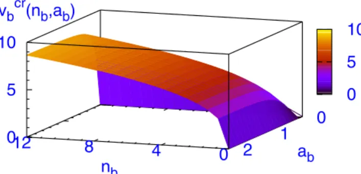
⳵_nb. 共13兲 In Fig.1we plot the critical sound velocityv_bcrof a uniform

Bose superfluid for the present␮b given by Eqs.共7兲and共8兲 with the parameter␯= 1.1. The interesting feature of this plot is that v_bcr= 0, when either n_b or a_b is zero. However, v_bcr

increases monotonically with nb, whereas v_bcrattains a

con-stant value asabincreases. These features are present in the plot of Fig. 1. However, the critical sound velocity v

b cr

cal-culated from ␮b given by Eqs. 共7兲 and共9兲increases mono-tonically with bothnbandab.

For superfluid fermions the healing length of Cooper pairs can be defined as

␰p= ប mpv_pcr

, 共14兲

where the critical velocity v

p cr

is related to the breaking of pairs through the formula

v

p cr

=

冑

冑

␮p 2

+兩⌬兩2 −␮p mp

, 共15兲

where兩⌬兩is the energy gap关2,44兴. We notice that in the deep BCS regime of weakly interacting attractive Fermi atoms 共corresponding to 兩⌬兩Ⰶ␮p兲 Eq. 共15兲 approaches the expo-nentially small value vcr_p=兩⌬兩/

冑

m_p␮_p/2.

III. NONLINEAR SCHRÖDINGER EQUATIONS

The bosonic superfluid can be described by a GP关1,25兴 complex order parameter⌿b共r,t兲given by

⌿b共r,t兲=

冑

nb共r,t兲ei␪b共r,t兲. 共16兲 The probability current densityជj共r,t兲is given by

j

ជ⬅nbvb= ប 2imb

共⌿_b*⵱_⌿b−⌿b⵱_⌿

b

*_{兲. 共17兲}

Equations共16兲and共17兲relate the phase␪b共r,t兲to the super-fluid velocity field vb by the formula关1兴

vb= ប mb

⵱_{␪b. 共18兲}

The bosonic order parameter ⌿b共r,t兲 is, apart from a nor-malization 关4,5兴, nothing but the condensate wave function

⌶b共r,t兲=具␺ˆ共r,t兲典, 共19兲 that is, the expectation value of the bosonic field operator

␺ˆ共r,t兲 关4,23兴. The order parameter⌿b共r,t兲 satisfies the fol-lowing generalized GP nonlinear Schrödinger equation 关1兴

iប⳵

⳵_t⌿b=

冉

− ប2 2mb

ⵜ2₊Ub+␮b共nb,ab兲

冊

⌿b, 共20兲 where the bulk chemical potential is given by Eq. 共7兲. The use of f共x兲= 4␲xin Eq.共7兲leads to the GP equation and the use of the two leading terms of Eq. 共9兲, e.g.,

f共x兲= 4␲

冉

x+ 32 3

冑␲

x

5/2

冊

_共

21兲

in Eq. 共7兲 leads to the modified GP 共MGP兲 equation sug-gested by Fabrocini and Polls关24兴, which includes correction to the GP equation for medium values of Bose-Bose scatter-ing length a_b. The use of Eq.共8兲in Eq. 共7兲leads to a

non-0

5

10

0

4

8

12

n

_b

0

1

2

a

_b

0

5

10

v

_bcr

(n

_b

,a

_b

)

FIG. 1. 共Color online兲The critical sound velocityv b cr

of a uni-form Bose superfluid as a function of Bose-Bose scattering length

linear Schrödinger equation valid from the weak-coupling to the unitarity limit and is called the unitary Schrödinger共US兲 equation for bosons关22兴.

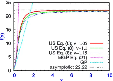
In Fig.2 we plot the various possibilities for the interpo-lation function f共x兲; e.g., those corresponding to the US equation共8兲with共a兲␯= 1.05,共b兲␯= 1.1, and共c兲␯= 1.15关as suggested after Eq. 共9兲兴, the MGP equation 共21兲, the GP equation f共x兲= 4␲x. The asymptotic limit limx→⬁f共x兲

= 22.22 is also shown. All three choices 共a兲, 共b兲, and 共c兲 represent smooth interpolation of f共x兲 between small and largexvalues. For smallxthis choice agrees with the MGP result共21兲and for largexwith the asymptotic result. To test these three choices we actually solve the US Eq. 共20兲, by imaginary time propagation after a Crank-Nicholson discreti-zation关45–47兴 共detailed in the beginning of Sec. IV兲, for the trap parameters of a possible experimental setup for 87Rb atoms in a spherical trap and compare the results for energy with those obtained by Blume and Greene关48兴by the diffu-sion Monte Carlo共DMC兲 method. Actually, we solved Eqs. 共20兲 and共7兲 withnb normalized to 共Nb− 1兲 in place of Eq. 共3兲, as appropriate for a small number of bosons, cf. Eq.共2兲 of 关48兴. The energy of the calculation is performed for a boson-boson scattering lengtha_b= 0.433lwherelis the har-monic oscillator length for various Nb and the results for energy are displayed in TableI. From this table we find that

the present US models always provide a much better ap-proximation to the energies than the GP and MGP models. More results of energy for larger number of bosons may help in fixing the parameters of the present model more accu-rately. In the present paper we shall use the US model 共b兲 with␯= 1.1.

The relationship between Eq.共20兲and the hydrodynami-cal equations共1兲and共2兲can be established by inserting Eq. 共16兲into Eq.共20兲. After some straightforward algebra equat-ing the real and imaginary parts of both sides and takequat-ing into account Eq.共18兲, one finds two generalized hydrodynamical equations 关1兴,

⳵

⳵_tnb+⵱·共nbvb兲= 0, 共22兲

mb ⳵

⳵tvb+⵱

冉

− ប2 2mb

ⵜ2

冑

_n b

冑

nb +mb

v_b2

2 +Ub+␮b共nb,ab兲

冊

= 0, 共23兲 which include the quantum pressure term

T_bQP= − ប 2

2mb ⵜ2

冑

nb

冑

nb

, 共24兲

which depends explicitly on the reduced Planck constantប. Neglecting the quantum pressure term, one gets from Eqs. 共22兲and共23兲the classical hydrodynamical equations共1兲and 共2兲. Equation 共22兲 is the continuity equation whereas Eq. 共23兲establishes the irrotational nature of hydrodynamic flow. Similarly, the fermionic superfluid can be described by a DF 关32兴 complex order parameter ⌿p共r,t兲 of pairs, with a modulus and a phase␪p共r,t兲such that

⌿p共r,t兲=

冑

np共r,t兲ei␪p共r,t兲. 共25兲 The expression for the probability current density of fermi-ons leads to the following expression for the velocity fieldv_p of pairs关2兴:

vp= ប mp

⵱␪p. 共26兲

Note that the mass of a pair mp, and not that of a fermion, appears in the denominator of the phase-velocity relation. The fundamental entity responsible for superfluid flow has the massm_pof a pair of fermions. For paired fermions in the superfluid state, the order parameter is, apart from a normal-0

5 10 15 20 25

0 2 4 6 8 10

f(

x

)

x

US Eq. (8);ν=1.05

0 5 10 15 20 25

0 2 4 6 8 10

f(

x

)

x

US Eq. (8);ν=1.05

US Eq. (8);ν=1.1

0 5 10 15 20 25

0 2 4 6 8 10

f(

x

)

x

US Eq. (8);ν=1.05

US Eq. (8);ν=1.1

US Eq. (8);ν=1.15

0 5 10 15 20 25

0 2 4 6 8 10

f(

x

)

x

US Eq. (8);ν=1.05

US Eq. (8);ν=1.1

US Eq. (8);ν=1.15

MGP Eq. (21)

0 5 10 15 20 25

0 2 4 6 8 10

f(

x

)

x

US Eq. (8);ν=1.05

US Eq. (8);ν=1.1

US Eq. (8);ν=1.15

MGP Eq. (21) GP

0 5 10 15 20 25

0 2 4 6 8 10

f(

x

)

x

US Eq. (8);ν=1.05

US Eq. (8);ν=1.1

US Eq. (8);ν=1.15

MGP Eq. (21) GP asymptotic: 22.22

FIG. 2. 共Color online兲 The Bose interpolation function f共x兲

given by Eq. 共8兲 with ␣= 32␯/_共3

冑

_{␲兲, ␥= 32共␯− 1兲}/_共3

冑

_{␲兲, and ␤} = 4␲␣/22.22 with␯=共a兲1.05,共b兲1.1, and共c兲1.15. The results of MGP 关Eq. 共21兲兴 and GP 关f共x兲= 4␲x兴 models together with the asymptotic value are also given.

TABLE I. Ground state energies for different numberN_bof bosonic atoms in a spherical trap and for

ab= 0.433 from a solution of GP equation, MGP equation, and US equation for␯=共a兲1.05,共b兲1.1, and共c兲

1.15. The results for energies obtained with two potentials of DMC calculation关48兴are quoted for compari-son. Length and energies are expressed in oscillator units.

N_b DMC GP MGP US共a兲 US共b兲 US共c兲

3 5.553共3兲; 5.552共2兲 5.329 5.611 5.570 5.564 5.558

5 10.577共2兲; 10.574共4兲 9.901 10.772 10.629 10.608 10.588

10 26.22共8兲; 26.20共8兲 23.61 26.84 26.24 26.16 26.07

ization关4,5,49兴, the condensate wave function of the center of mass of the Cooper pairs:

⌶p共r,t兲=具␺ˆ↑共r,t兲␺ˆ↓共r,t兲典, 共27兲

that is the average of pair operators, with␺ˆ

␴共r,t兲the

fermi-onic field operator with spin component␴=↑,↓ 关4,23兴. The order parameter ⌿p共r,t兲 satisfies the following zero-temperature nonlinear DF Schrödinger equation 关23,28,29,31,39兴:

iប⳵

⳵t⌿p=

冉

− ប2 2m_pⵜ

2_+U

p+␮p共np,af兲

冊

⌿p, 共28兲 where the bulk chemical potential␮p共np,af兲 is given by Eq. 共10兲. The use ofg共x兲= 1 in␮_p共n_p,a_f兲of Eq.共10兲leads to the lowest order DF equation. If we use the next order solution of Eq.共11兲in Eq.共10兲, e.g.,

g共x兲= 1 +␦x, 共29兲 we obtain a modified density-functional 共MDF兲 equation with corrections for medium value Fermi-Fermi scattering length af. The use of Eq. 共11兲 in Eq. 共10兲 leads to a DF equation valid in the weak-coupling BCS to unitarity limit and the resultant nonlinear equation 共28兲 will be called the unitary Schrödinger共US兲equation for fermion pairs.

In Fig.3 we plot the various possibilities for the interpo-lation functiong共x兲; e.g., that corresponding to Eq.共11兲, the MDF equation 共29兲 for two different values of ␦: 共i兲 4␲/共_3␲2兲2/3 _and 共_ii兲 _20␲/共_3␲2兲2/3_{. The parameter} ␬ _is

al-ways taken as ␬=␦/共_{1 −␨}兲_{,␨= 0.44} 关_40,41兴_{. The asymptotic}

limit limx→−⬁g共x兲= 0.44 is also shown in Fig.3. The

expres-sion共11兲represents a good approximation ofg共x兲for small and large 兩x兩. For small兩x兩 this choice agrees with the MDF result 共29兲 and for large 兩x兩 with the asymptotic result for both choices of␦.

To test the above two choices共i兲and共ii兲of the parameter

␦ in Eq.共11兲 for a Fermi superfluid in a spherical trap, we calculate the energy of the system for different values of the scattering length a_f and number of atoms N_f by solving di-rectly Eq.共28兲by imaginary time propagation after a Crank-Nicholson discretization 关45–47兴 共detailed in the beginning

of Sec. IV兲. We also compare the results with those obtained by the fixed-node Monte Carlo calculation共FNMC兲 关50–53兴. The results of our investigation are shown in Figs.4. In Fig. 4共a兲we plot energy Evs兩a_f兩 forN_f= 4 and 8 obtained from a solution the US equation 共28兲 with the choices 共i兲 4␲/_共3␲2_兲2/3_{and共ii兲20␲}/_共3␲2_兲2/3_{for␦and the FNMC data}

of Refs. 关52,53兴. The present hydrodynamical formulation is expected to be good for a large number of fermions 关see, Fig.4共b兲兴, yet for a small numberN_f= 4 the result is reason-able. In Fig. 4共b兲we plot energyE/_N

f 2/3

vsN_f2/3 at unitarity af→−⬁ obtained from a solution of the US equation 共28兲 with choice共ii兲20␲/共_3␲2兲2/3_for␦_{. In this limit both choices}

of␦ lead to the same energy. The results of FNMC关50兴and Green function Monte Carlo 共GFMC兲 关54兴 calculations as well as of local density approximation共LDA兲are also shown in Fig. 4共b兲. The LDA result is analytically known in this case asE共N兲=共3Nf兲4/3

冑

␰/4,␰= 0.44关33兴. We plotE/Nf

2/3 vs N_f2/3 in Fig. 4共b兲 because of the linear correlation between these two variables explicit in the LDA result. From Figs. 4 we find that the results with choice 共ii兲 20␲/_共3␲2_兲2/3 _of ␦

0.4 0.5 0.6 0.7 0.8 0.9 1

-10 -8 -6 -4 -2 0

g

(x

)

x US Eq. (11) (i)

0.4 0.5 0.6 0.7 0.8 0.9 1

-10 -8 -6 -4 -2 0

g

(x

)

x US Eq. (11) (i) MDF Eq. (29) (i)

0.4 0.5 0.6 0.7 0.8 0.9 1

-10 -8 -6 -4 -2 0

g

(x

)

x US Eq. (11) (i) MDF Eq. (29) (i) US Eq. (11) (ii)

0.4 0.5 0.6 0.7 0.8 0.9 1

-10 -8 -6 -4 -2 0

g

(x

)

x US Eq. (11) (i) MDF Eq. (29) (i) US Eq. (11) (ii) MDF Eq. (29) (ii)

0.4 0.5 0.6 0.7 0.8 0.9 1

-10 -8 -6 -4 -2 0

g

(x

)

x US Eq. (11) (i) MDF Eq. (29) (i) US Eq. (11) (ii) MDF Eq. (29) (ii) asymptotic: 0.44

FIG. 3. 共Color online兲 The Fermi interpolation function g共x兲

given by Eq.共11兲with共i兲␦= 4␲/共3␲2_兲2/₃

and共ii兲20␲/共3␲2_兲2/₃

and

␬=␦/_{0.56. The MDF results given by Eq.共29兲and the asymptotic} value are also shown.

10 15 20

0.001 0.01 0.1 1 10 100 1000

E

|a_f| X 2

US (N_f=8) (ii)

10 15 20

0.001 0.01 0.1 1 10 100 1000

E

|a_f| X 2

US (N_f=8) (ii) US (N_f=8) (i)

10 15 20

0.001 0.01 0.1 1 10 100 1000

E

|a_f| X 2

US (N_f=8) (ii) US (N_f=8) (i) FNMC (N_f=8)

10 15 20

0.001 0.01 0.1 1 10 100 1000

E

|a_f| X 2

US (N_f=8) (ii) US (N_f=8) (i) FNMC (N_f=8) US (N_f=4) (ii)

10 15 20

0.001 0.01 0.1 1 10 100 1000

E

|a_f| X 2

US (N_f=8) (ii) US (N_f=8) (i) FNMC (N_f=8) US (N_f=4) (ii) FNMC (N_f=4)

0 2 4 6 8

0 2 4 6 8 10

E/N

f

2/3

N_f2/3

US

0 2 4 6 8

0 2 4 6 8 10

E/N

f

2/3

N_f2/3

US FNMC

0 2 4 6 8

0 2 4 6 8 10

E/N

f

2/3

N_f2/3

US FNMC GFMC

0 2 4 6 8

0 2 4 6 8 10

E/N

f

2/3

N_f2/3

US FNMC GFMC LDA

(b) (a)

FIG. 4. 共Color online兲 共a兲Energy of a superfluid Fermi gas in a spherical trap in oscillator units vs Fermi-Fermi scattering lengthaf

also in oscillator units obtained from the solution of Eq.共28兲for the choices␦=共i兲4␲/_共3␲2_兲2/3_{and共ii兲20␲/共3␲}2_兲2/3_{and from the fixed}

node Monte Carlo 共FNMC兲 calculation 关52,53兴. 共b兲 Energy of a superfluid Fermi gas in a spherical trap in oscillator units vs number of atomsNfin the unitarity limitaf→−⬁obtained from a solution

of Eq. 共28兲, from FNMC 关50兴 and Green function Monte Carlo

共GFMC兲 calculations 关54兴, and from local density approximation

agree well with the Monte Carlo data in both cases and this choice will be used in the present study. The Monte Carlo data clearly favor the present model over the LDA.

Again, inserting Eq. 共25兲 into Eq. 共28兲, after some straightforward algebra equating the real and imaginary parts and taking into account Eq. 共26兲, we find two generalized hydrodynamical equations for the Fermi superfluid,

⳵

⳵_tnp+⵱·共npvp兲= 0, 共30兲

mp ⳵

⳵_tvp+⵱

冋

− ប2 2mp

ⵜ2

冑

np

冑

np +mp

v

p 2

2 +Up+␮p共np,af兲

册

= 0, 共31兲

which include the quantum pressure term

T_pQP= − ប 2

2mp ⵜ2

冑

_n

p

冑

n_p , 共32兲

involving ប. Neglecting this term leads to the classical hy-drodynamical equations共4兲and共5兲of superfluid Fermi pairs. This specific quantum pressure term is a consequence of the proper phase-velocity relation共26兲with the factormp in the denominator关2兴. Had we taken a different mass factor in the denominator, e.g., mf, a different quantum pressure term would have emerged. The present choice is physically moti-vated by Galilei invariance关2,23,31兴and leads to energies of trapped Fermi superfluid in close agreement关55兴with those obtained关50,54兴from the Monte Carlo methods.

We stress that, from the point of view of DF theory, the quantum pressure terms for superfluid bosons and fermions correspond to gradient correction共also called surface correc-tions兲to the local density approximation共LDA兲, where LDA gives exactly the classical hydrodynamical equations ob-tained by setting the gradient kinetic-energy term to zero. The gradient term, which can also be seen as a next-to-leading contribution in a momentum expansion to the classi-cal superfluid hydrodynamics关56兴, takes into account correc-tions to the kinetic energy due to spatial variacorrec-tions in the density of the system, and it is essential to have regular be-havior at the surface of the cloud where the density goes to zero 关57兴. In the case of superfluid bosons, the quantum-pressure term, Eq. 共24兲, is exactly the one of the familiar cubic GP equation关1,25兴. In the case of superfluid fermions the gradient term is consistent with the motion of paired fermions of massmp= 2mf. For normal fermions various au-thors have proposed and used different gradient terms 关57–61兴. For superfluid fermions we are using the familiar von Weizsäcker term关58兴in the case of pairs. In fact, in our approach, the explicit form of the quantum-pressure term, Eq. 共32兲, is strictly determined by the Galilei-invariant rela-tion, Eq. 共26兲, between phase and superfluid velocity 关2,23,31兴. Finally, we observe that Eq.共32兲is practically the same as that recently obtained in Ref. 关62兴 in the case of a superfluid Fermi gas at unitarity using an⑀expansion around d= 4 −⑀spatial dimensions.

The generalized hydrodynamical equations共22兲 and共23兲 for bosons and Eqs.共30兲and共31兲for fermions are thus com-pletely equivalent to the respective nonlinear Schrödinger equations 共20兲and共28兲. In the limit of zero velocity fields, v_b,v_p→0, Eqs.共23兲and共31兲yield the stationary versions of Eqs. 共20兲and共28兲describing the superfluid densities:

␮b0

冑

nb=

冉

− ប2 2m_bⵜ

2

+U_b+␮b共nb,ab兲

冊

冑

nb, 共33兲

␮p0

冑

np=

冉

− ប2 2m_pⵜ

2_+U

p+␮p共np,af兲

冊

冑

np, 共34兲 showing the agreement between hydrodynamical and nonlin-ear equations for superfluid bosons and fermions. Here ␮b0 and␮p0are the chemical potentials for bosons and fermions in the stationary state.

Although Eq. 共34兲is written in terms of Fermi pair den-sity np 共and we use this equation in the following兲, an equivalent equation for Fermi densityn_f共=2n_p兲can be writ-ten as

␮_f0

冑

n_f=

冉

− ប 2

8mf

ⵜ2₊U_f+␮_f共n_f,a_f兲

冊

冑

n_f, 共35兲

␮f共nf,af兲= ប2 2m_f共3␲

2_n f兲2

/3_g共n f 1/3_a

f兲, 共36兲 where we have used ␮p0= 2␮f0, Up= 2Uf, and ␮p共np,af兲 = 2␮_f共n_f,a_f兲.

Equations共20兲and共28兲are the Euler-Lagrange equations of the following Lagrangian density:

L_j=iប 2

冉

⌿*j

⳵

⳵t⌿j−⌿j ⳵

⳵t⌿j*

冊

− ប2 2m_j兩⵱⌿j兩

2_−U j共r兲兩⌿j兩2 −Ej共nj,aj兲兩⌿j兩2, 共37兲 with j=b,p 共herea_p=a_f, the Fermi-Fermi scattering length兲 where

Ej共nj,aj兲= 1 nj

冕

0

n_j

␮j共nj

⬘

,aj兲dnj

⬘

, 共38兲

is the bulk energy per particle of the superfluid.

Finally, we introduce a Lagrangian density for Bose-Fermi interaction to Eq.共37兲of the form

Lbp=Gbp兩⌿b兩2兩⌿p兩2, 共39兲 whereG_bp= 4␲ប2_a

bf/mbf, andmbfis the Bose-Fermi reduced mass andabfis the Bose-Fermi scattering length.

We note that there are no coupling terms between the hydrodynamical equations共23兲and共31兲involving the veloc-ity of two superfluid components. The only coupling in the Lagrangian density共39兲 involves the density of the two su-perfluid components. However, the present hydrodynamical equations 共23兲and共31兲 are a special case of the three-fluid 共two superfluids and a normal fluid兲hydrodynamical formu-lation of Landau and Khalatnikov 关63兴 共appropriate for the 4

in-volving two superfluid velocities共not considered in this pa-per兲, as discussed关64兴by Andreev and Bashkin and also by Ho and Shenoy. However, the present static model defined by Eqs. 共33兲 and 共34兲 is obtained by setting all velocities equal to zero, and hence these terms depending on superfluid velocities would leave the present model unchanged.

In this paper we considerabfto have not too large positive values only 共moderately repulsive Bose-Fermi interaction兲. There are other domains of Bose-Fermi interaction which require special attention. If this interaction is attractive and strong enough, then the ground state is very different, e.g., the composite fermions f˜=bf are created at higher tempera-tures and at zero temperature we have Cooper pairs共or local pairs兲of the type具f˜f˜典consisting of two elementary fermions and two elementary bosons关65兴.

The complete Lagrangian density given by Eqs.共37兲and 共39兲 leads to the following set of coupled equations for the Bose-Fermi-Fermi mixture made of superfluid bosons and two-component superfluid fermions:

iប⳵

⳵_t⌿b=

冉

− ប2_ⵜ2

2mb

+Ub+␮b共nb,ab兲+Gbp兩⌿p兩2

冊

⌿b, 共40兲

iប⳵

⳵_t⌿p=

冉

− ប2_ⵜ2

2mp

+Up+␮p共np,af兲+Gbp兩⌿b兩2

冊

⌿p, 共41兲 valid from weak-coupling to unitarity for both bosons and fermions. The coupled set of equations 共40兲 and 共41兲 with bulk chemical potentials ␮_b共n_b,a_b兲 and ␮_p共n_p,a_f兲 given by Eqs. 共7兲 and共8兲 共with␯= 1.1兲 and Eqs.共10兲 and共11兲 关with

␦= 20␲/_共3␲2_兲2/3_{, ␬=␦}/_{共1 −␨兲, ␨= 0.44兴, respectively, is the}

US equation for the interacting superfluid Bose-Fermi mix-ture and is the required set. However, when the bulk chemi-cal potentials ␮b共nb,ab兲and␮p共np,af兲are approximated us-ing Eqs.共21兲and共29兲, the set of equations共40兲and共41兲will be termed modified Gross-Pitaevskii density-functional 共MGPDF兲 equation including some correction for medium values of scattering lengthsabandaf. Finally, if we approxi-mate f共x兲= 4␲xandg共x兲= 1 in Eqs.共40兲and共41兲 with Eqs. 共8兲 and 共11兲, the resultant model is termed the Gross-Pitaevskii density-functional 共GPDF兲 model. We present a comparative numerical study of these three models—US, MGPDF, and GPDF—in the next section.

IV. NUMERICAL RESULTS

Here we solve numerically the coupled set of US Eqs. 共40兲and共41兲with bulk chemical potentials␮band␮pgiven by Eqs.共8兲and共11兲and compare the results so obtained with those of the MGPDF and GPDF models. We numerically solve the US, MGPDF, and GPDF partial differential equa-tions by discretizing them by the semi-implicit Crank-Nicholson algorithm with imaginary time propagation 关45–47兴. The space and time steps used in discretization were typically 0.05 and 0.001, respectively.

Although we are not interested here in fitting experimen-tal data, we perform numerical calculation for variables for a

possible experimental setup 关16兴 of a 87Rb-40K mixture in spherical harmonic traps satisfying U_b=m_b␻_b2_r2_/2 =mf␻f

2_r2_{/2 =U}

f with an oscillator length l=

冑

ប/共mb␻b兲 = 1␮m for 87Rb atoms. The oscillator length for 40K is modified according to the trap. The fermion pair trap in Eq. 共41兲isUp=mf␻f

2_r2_.

In Figs.5共a兲and5共b兲we plot densities for the superfluid Bose-Fermi mixture as calculated from Eqs. 共40兲 and 共41兲 for Nb= 10 000,Np= 10 000, af= 0,abf= 100 nm with 共a兲 ab = 200 nm and 共b兲 ab= 2000 nm for the US, MGPDF, and GPDF models. For small a_b both MGPDF, and GPDF mod-els are good approximations to the bosonic density of the US model 共not shown in the figure兲. But as ab increases, the MGPDF model is a better approximation to the bosonic den-sity of the US model than the GPDF model as can be seen from Fig.5共a兲. However, for very large a_b, neither the MG-PDF nor the GMG-PDF model provides the saturation of bulk chemical potential for bosons as in the US model. Conse-quently, the MGPDF and GPDF models acquire large bosonic nonlinearity compared to the US model and hence produce bosonic density extending to a larger region in space. Asab is increased, the MGPDF model yields rapidly divergent bosonic nonlinearity 共compared to the GPDF model兲 and hence produces bosonic density inferior to the GPDF model as can be seen in Fig.5共b兲.

In Figs. 6共a兲 and 6共b兲 we plot superfluid densities for Nb= 100 000, Np= 100, abf= 100 nm, ab= 5 nm with 共a兲 af = −100 nm and 共b兲 af= −300 nm for the US, MGPDF, and

0 0.0004 0.0008 0.0012

0 2 4 6 8 10 12 14 16

nj

(r)

r (µm)

N_b=10000 N_p=10000 a_bf=100 nm a_b=200 nm a_f=0 nm

n_b, US

0 0.0004 0.0008 0.0012

0 2 4 6 8 10 12 14 16

nj

(r)

r (µm)

N_b=10000 N_p=10000 a_bf=100 nm a_b=200 nm a_f=0 nm

n_b, US n_p, US

0 0.0004 0.0008 0.0012

0 2 4 6 8 10 12 14 16

nj

(r)

r (µm)

N_b=10000 N_p=10000 a_bf=100 nm a_b=200 nm a_f=0 nm

n_b, US n_p, US n_b, MGPDF

0 0.0004 0.0008 0.0012

0 2 4 6 8 10 12 14 16

nj

(r)

r (µm)

N_b=10000 N_p=10000 a_bf=100 nm a_b=200 nm a_f=0 nm

n_b, US n_p, US n_b, MGPDF n_p, MGPDF

0 0.0004 0.0008 0.0012

0 2 4 6 8 10 12 14 16

nj

(r)

r (µm)

N_b=10000 N_p=10000 a_bf=100 nm a_b=200 nm a_f=0 nm

n_b, US n_p, US n_b, MGPDF n_p, MGPDF n_b, GPDF

0 0.0004 0.0008 0.0012

0 2 4 6 8 10 12 14 16

nj

(r)

r (µm)

N_b=10000 N_p=10000 a_bf=100 nm a_b=200 nm a_f=0 nm

n_b, US n_p, US n_b, MGPDF n_p, MGPDF n_b, GPDF n_p, GPDF

0 0.0002 0.0004 0.0006 0.0008

0 2 4 6 8 10 12 14 16 18 20

nj

(r

)

r (µm)

N_b=10000 N_p=10000 a_bf=100 nm a_b=2000 nm a_f=0 nm

n_b, US

0 0.0002 0.0004 0.0006 0.0008

0 2 4 6 8 10 12 14 16 18 20

nj

(r

)

r (µm)

N_b=10000 N_p=10000 a_bf=100 nm a_b=2000 nm a_f=0 nm

n_b, US n_p, US

0 0.0002 0.0004 0.0006 0.0008

0 2 4 6 8 10 12 14 16 18 20

nj

(r

)

r (µm)

N_b=10000 N_p=10000 a_bf=100 nm a_b=2000 nm a_f=0 nm

n_b, US n_p, US n_b, MGPDF

0 0.0002 0.0004 0.0006 0.0008

0 2 4 6 8 10 12 14 16 18 20

nj

(r

)

r (µm)

N_b=10000 N_p=10000 a_bf=100 nm a_b=2000 nm a_f=0 nm

n_b, US n_p, US n_b, MGPDF n_p, MGPDF

0 0.0002 0.0004 0.0006 0.0008

0 2 4 6 8 10 12 14 16 18 20

nj

(r

)

r (µm)

N_b=10000 N_p=10000 a_bf=100 nm a_b=2000 nm a_f=0 nm

n_b, US n_p, US n_b, MGPDF n_p, MGPDF n_b, GPDF

0 0.0002 0.0004 0.0006 0.0008

0 2 4 6 8 10 12 14 16 18 20

nj

(r

)

r (µm)

N_b=10000 N_p=10000 a_bf=100 nm a_b=2000 nm a_f=0 nm

n_b, US n_p, US n_b, MGPDF n_p, MGPDF n_b, GPDF n_p, GPDF

(b) (a)

FIG. 5. 共Color online兲 The normalized densities n_j共r兲=兩⌿j兩2

withj=b,pfrom a solution of Eqs.共40兲and共41兲for the US, MG-PDF, and GPDF models with N_b= 10 000, N_p= 10 000, a_bf

= 100 nm,af= 0, and共a兲ab= 200 nm, and共b兲ab= 2000 nm. In this

GPDF models. For small兩af兩 the fermionic densities of both MGPDF and GPDF models are a good approximation to the US model. But as兩a_f兩 increases, the GPDF model continues with BCS nonlinearity foraf= 0, whereas the fermionic non-linearity of the MGPDF model acquires excessive attraction. This is clear from Figs. 6共a兲 and 6共b兲 showing a peaked fermionic density for the MGPDF model for large兩af兩 corre-sponding to increased attraction. For very large兩a_f兩, the MG-PDF model does not provide the saturation of fermionic bulk chemical potential as in the US model. We note that com-pared to the study of Figs. 5 with comparable number of bosons and fermions, in the study of Figs.6we have a much reduced number of fermions compared to bosons and the system has undergone a mixing-demixing transition 关20,66兴 expelling the fermions from the central to the peripheral re-gion.

Next we calculate the chemical potentials␮_b0and␮_p0of the stationary superfluid Bose-Fermi mixture as described by Eqs. 共33兲 and 共34兲. In Figs. 7共a兲 and 7共b兲 we plot these chemical potentials under the situations described in Figs.4 and 5, e.g., in the 共a兲 weak-coupling BCS limit when ab varies from a small to a large value and共b兲weak-coupling GP limit when 兩af兩 varies from a small to a large value, respectively. In the first case the fermionic chemical potential

␮p0remains practically constant over the full range of varia-tion of ab and we plot only the bosonic chemical potential

␮b0in Fig.7共a兲. In the second case bosonic chemical

poten-tial ␮b0 remains practically constant over the full range of variation ofafand we plot only the fermionic chemical po-tential ␮p0. From Fig. 7共a兲we find that, although for small values ofab, the MGPDF model produces results for␮b0in close agreement with the US model, for medium values ofab the GPDF model produces results closer to the US model. However, for larger values ofabthe US model should show saturation, whereas the GPDF chemical potential␮b0should increase monotonically withaband should be larger than the chemical potential of the US model 共not shown in figure兲. From Fig. 7共b兲we find that none of the MGPDF or GPDF models produces a reasonable result for␮p0except for very small values of 兩af兩. The GPDF model does not have a de-pendence onafand hence produces a constant result for␮p0.

V. CONCLUSION

The dynamics of cold trapped atoms 共both bosons and fermions兲should be correctly handled by a proper treatment of many-body dynamics or through a field-theoretic formu-lation. However, both approaches could be much too com-plicated to have an advantage in phenomenological applica-tion. This is why mean-field approaches are widely used for phenomenological application. In the weak-coupling limit, for bosonic atoms the dynamics is handled through the mean-field GP equation关1兴, whereas for fermionic atoms the

0 0.001 0.002 0.003 0.004

0 2 4 6 8

nj

(r

)

r (µm)

N_b=100000

N_p=100

a_bf=100 nm

a_b=5 nm

a_f=-100 nm

n_b, US

0 0.001 0.002 0.003 0.004

0 2 4 6 8

nj

(r

)

r (µm)

N_b=100000

N_p=100

a_bf=100 nm

a_b=5 nm

a_f=-100 nm

n_b, US n_p, US

0 0.001 0.002 0.003 0.004

0 2 4 6 8

nj

(r

)

r (µm)

N_b=100000

N_p=100

a_bf=100 nm

a_b=5 nm

a_f=-100 nm

n_b, US n_p, US n_b, MGPDF

0 0.001 0.002 0.003 0.004

0 2 4 6 8

nj

(r

)

r (µm)

N_b=100000

N_p=100

a_bf=100 nm

a_b=5 nm

a_f=-100 nm

n_b, US n_p, US n_b, MGPDF n_p, MGPDF

0 0.001 0.002 0.003 0.004

0 2 4 6 8

nj

(r

)

r (µm)

N_b=100000

N_p=100

a_bf=100 nm

a_b=5 nm

a_f=-100 nm

n_b, US n_p, US n_b, MGPDF n_p, MGPDF n_b, GPDF

0 0.001 0.002 0.003 0.004

0 2 4 6 8

nj

(r

)

r (µm)

N_b=100000

N_p=100

a_bf=100 nm

a_b=5 nm

a_f=-100 nm

n_b, US n_p, US n_b, MGPDF n_p, MGPDF n_b, GPDF n_p, GPDF

0 0.001 0.002 0.003 0.004

0 2 4 6 8

nj

(r

)

r (µm)

N_b=100000

N_p=100

a_bf=100 nm

a_b=5 nm

a_f=-300 nm

n_b, US

0 0.001 0.002 0.003 0.004

0 2 4 6 8

nj

(r

)

r (µm)

N_b=100000

N_p=100

a_bf=100 nm

a_b=5 nm

a_f=-300 nm

n_b, US n_p, US

0 0.001 0.002 0.003 0.004

0 2 4 6 8

nj

(r

)

r (µm)

N_b=100000

N_p=100

a_bf=100 nm

a_b=5 nm

a_f=-300 nm

n_b, US n_p, US n_b, MGPDF

0 0.001 0.002 0.003 0.004

0 2 4 6 8

nj

(r

)

r (µm)

N_b=100000

N_p=100

a_bf=100 nm

a_b=5 nm

a_f=-300 nm

n_b, US n_p, US n_b, MGPDF n_p, MGPDF

0 0.001 0.002 0.003 0.004

0 2 4 6 8

nj

(r

)

r (µm)

N_b=100000

N_p=100

a_bf=100 nm

a_b=5 nm

a_f=-300 nm

n_b, US n_p, US n_b, MGPDF n_p, MGPDF n_b, GPDF

0 0.001 0.002 0.003 0.004

0 2 4 6 8

nj

(r

)

r (µm)

N_b=100000

N_p=100

a_bf=100 nm

a_b=5 nm

a_f=-300 nm

n_b, US n_p, US n_b, MGPDF n_p, MGPDF n_b, GPDF n_p, GPDF

(b) (a)

FIG. 6. 共Color online兲 The normalized densities n_j共r兲=兩⌿j兩2

withj=b,pfrom a solution of Eqs.共40兲and共41兲for the US, MG-PDF, and GPDF models withN_b= 100 000,N_p= 100,a_bf= 100 nm,

ab= 5 nm, and共a兲af= −100 nm, and共b兲abf= −300 nm. In this plot 兰nj共r兲d3r= 1.

0 20 40 60 80

0 200 400 600 800 1000

µb0

a_b(nm) N_b=10000 N_p=10000 a_bf=100 nm a_f=0 nm _US

0 20 40 60 80

0 200 400 600 800 1000

µb0

a_b(nm) N_b=10000 N_p=10000 a_bf=100 nm a_f=0 nm _US

MGPDF 0 20 40 60 80

0 200 400 600 800 1000

µb0

a_b(nm) N_b=10000 N_p=10000 a_bf=100 nm a_f=0 nm _US

MGPDF GPDF 50 52 54 56

-1000 -800 -600 -400 -200 0

µp0

a_f(nm) N_b=100000 N_p=100 a_bf=100 nm a_b=5 nm

US

50 52 54 56

-1000 -800 -600 -400 -200 0

µp0

a_f(nm) N_b=100000 N_p=100 a_bf=100 nm a_b=5 nm

US MGPDF 50 52 54 56

-1000 -800 -600 -400 -200 0

µp0

a_f(nm) N_b=100000 N_p=100 a_bf=100 nm a_b=5 nm

US MGPDF GPDF

(b) (a)

FIG. 7. 共Color online兲 共a兲Chemical potential␮b0vsabof Eqs. 共33兲 and共34兲 for the US, MGPDF, and GPDF models forNb=Np

= 10 000, a_f= 0,a_bf= 100 nm and共b兲 chemical potential␮_p0vsa_f

for the US, MGPDF, and GPDF models forNb= 100 000,Np= 100, ab= 5 nm, abf= 100 nm, respectively. The chemical potentials are

LDA 共local density approximation兲 formulation is widely used关2兴. The LDA approach共often called the Thomas-Fermi approximation兲lacks the kinetic energy gradient term共 quan-tum pressure term兲. Here we introduce a quantum pressure term consistent with the correct phase-velocity relation of the superfluid fermions assuring the Galilei invariance of the model 关23兴. This modified LDA equation for fermions and the GP equation for bosons, both valid in the weak-coupling limit, are both shown to be equivalent to the hydrodynamical equation for superfluid flow. In the strong-coupling unitarity limit as the bosonic and fermionic scattering lengthsa_b and 兩af兩 tend to infinity, both the bosonic and fermionic interac-tions are to exhibit saturation due to constraints of quantum mechanics. We introduce proper unitarity saturation effects in these equations. In addition in our Bose-Fermi formulation we introduce a not too strong contact interaction between bosons and fermions. The resultant superfluid Bose-Fermi dynamics is described by a set of coupled partial differential equations, which is the principal result of this paper. In the time-dependent form with a Bose-Fermi interaction this set is described by Eqs.共40兲and共41兲with the stationary version without Bose-Fermi interaction given by Eqs.共33兲and共34兲. The present model for the superfluid Bose-Fermi mixture is termed the US model, valid in both weak- and strong-coupling unitarity limits for bosons and fermions. We also consider a model called the GPDF model where the boson

dynamics is handled by the GP Lagrangian and the fermion dynamics is handled by the LDA formulation with a proper kinetic energy gradient term. Finally, we also consider an-other model called the MGPDF model including lowest or-der correction to the GPDF model due to the nonzero bosonic and fermionic scattering lengths ab and兩af兩. How-ever, the MGPDF model does not provide a saturation of the nonlinear interaction in the unitarity limit when ab and兩af兩 tend to infinity. In our numerical studies of a87Rb-40K mix-ture in a spherical harmonic trap, we find that for medium interactions the MGPDF model produces improved results. However, for stronger interactions the full US model should be used. Although slightly complicated for analytic applica-tions, the present US model is no more complicated than the usual GP and LDA equations for numerical treatment and is expected to find wide applications in future studies of Bose-Fermi superfluid mixture.

ACKNOWLEDGMENTS

We thank D. Blume for kindly providing additional data of FNMC calculation 关53兴. S.K.A. has been partially sup-ported by the FAPESP and CNPq of Brazil. L.S. has been partially supported by the Fondazione CARIPARO and GNFM-INdAM.

关1兴L. Pitaevskii and S. Stringari, Bose-Einstein Condensation 共Oxford University Press, Oxford, 2003兲; F. Dalfovo, S. Giorgini, L. Pitaevskii, and S. Stringari, Rev. Mod. Phys. 71, 463共1999兲; C. J. Pethick and H. Smith,Bose-Einstein Conden-sation in Dilute Gases 共Cambridge University Press, Cam-bridge, England, 2002兲.

关2兴S. Giorgini, L. P. Pitaevskii, and S. Stringari, e-print arXiv:0706.3360, Rev. Mod. Phys.共to be published兲.

关3兴L. D. Landau and E. M. Lifshitz,Fluid Mechanics, Course of Theoretical Physics No. 6共Pergamon Press, London, 1987兲.

关4兴L. D. Landau and E. M. Lifshitz, Statistical Physics, Part 2: Theory of the Condensed State, Course of Theoretical Physics No. 9共Pergamon Press, London, 1987兲.

关5兴A. J. Leggett,Quantum Liquids共Oxford University Press, Ox-ford, 2006兲.

关6兴K. Mölmer, Phys. Rev. Lett. 80, 1804共1998兲.

关7兴N. Nygaard and K. Mølmer, Phys. Rev. A 59, 2974共1999兲.

关8兴M. J. Bijlsma, B. A. Heringa, and H. T. C. Stoof, Phys. Rev. A

61, 053601共2000兲.

关9兴H. Heiselberg, C. J. Pethick, H. Smith, and L. Viverit, Phys. Rev. Lett. 85, 2418共2000兲.

关10兴L. Viverit, C. J. Pethick, and H. Smith, Phys. Rev. A 61, 053605共2000兲.

关11兴L. Viverit, Phys. Rev. A 66, 023605共2002兲.

关12兴K. K. Das, Phys. Rev. Lett. 90, 170403共2003兲.

关13兴X. J. Liu, M. Modugno, and H. Hu, Phys. Rev. A 68, 053605

共2003兲; S. T. Chui and V. N. Ryzhov,ibid. 69, 043607共2004兲; S. K. Adhikari,ibid. 70, 043617共2004兲.

关14兴D. W. Wang, Phys. Rev. Lett. 96, 140404共2006兲.

关15兴G. Roati, F. Riboli, G. Modugno, and M. Inguscio, Phys. Rev. Lett. 89, 150403共2002兲.

关16兴M. Modugno, F. Ferlaino, F. Riboli, G. Roati, G. Modugno, and M. Inguscio, Phys. Rev. A 68, 043626共2003兲.

关17兴C. Ospelkaus, S. Ospelkaus, K. Sengstock, and K. Bongs, Phys. Rev. Lett. 96, 020401共2006兲.

关18兴L. Salasnich and F. Toigo, Phys. Rev. A 75, 013623共2007兲.

关19兴L. Salasnich, S. K. Adhikari, and F. Toigo, Phys. Rev. A 75, 023616共2007兲.

关20兴S. K. Adhikari and L. Salasnich, Phys. Rev. A 75, 053603

共2007兲.

关21兴K. M. O’Hara, S. L. Hemmer, S. R. Granade, M. E. Gehm, J. E. Thomas, V. Venturi, E. Tiesinga, and C. J. Williams, Phys. Rev. A 66, 041401共R兲 共2002兲; K. Dieckmann, C. A. Stan, S. Gupta, Z. Hadzibabic, C. H. Schunck, and W. Ketterle, Phys. Rev. Lett. 89, 203201共2002兲; C. A. Regal, M. Greiner, and D. S. Jin,ibid. 92, 083201共2004兲; S. Inouye, M. R. Andrews, J. Stenger, H. J. Miesner, D. M. Stamper-Kurn, and W. Ketterle, Nature共London兲 392, 151共1998兲.

关22兴S. K. Adhikari and L. Salasnich, Phys. Rev. A 77, 033618

共2008兲.

关23兴L. Salasnich, e-print arXiv:0804.1277.

关24兴A. Fabrocini and A. Polls, Phys. Rev. A 60, 2319共1999兲; 64, 063610共2001兲.

关25兴E. P. Gross, Nuovo Cimento 20, 454共1961兲; L. P. Pitaevskii, Zh. Eksp. Teor. Fiz. 40, 646共1961兲 关Sov. Phys. JETP 13, 451

共1961兲兴.

E. K. U. Gross,Density Functional Theory: An Approach to the Quantum Many-Body Problem共Springer, Berlin, 1990兲.

关27兴W. Kohn and L. J. Sham, Phys. Rev. 140, A1133共1965兲.

关28兴Y. E. Kim and A. L. Zubarev, Phys. Lett. A 327, 397共2004兲; Phys. Rev. A 70, 033612共2004兲.

关29兴N. Manini and L. Salasnich, Phys. Rev. A 71, 033625共2005兲; G. Diana, N. Manini, and L. Salasnich, ibid. 73, 065601

共2006兲; L. Salasnich and N. Manini, Laser Phys. 17, 169

共2007兲.

关30兴S. K. Adhikari and B. A. Malomed, Europhys. Lett. 79, 50003

共2007兲; Phys. Rev. A 76, 043626共2007兲.

关31兴L. Salasnich, N. Manini, and F. Toigo, Phys. Rev. A 77, 043609共2008兲.

关32兴L. N. Oliveira, E. K. U. Gross, and W. Kohn, Phys. Rev. Lett.

60, 2430共1988兲.

关33兴A. Bulgac, Phys. Rev. A 76, 040502共R兲 共2007兲.

关34兴D. M. Eagles, Phys. Rev. 186, 456共1969兲; A. J. Leggett, J. Phys. 共Paris兲, Colloq. 41, C7-19 共1980兲; P. Nozières and S. Schmitt-Rink, J. Low Temp. Phys. 59, 195共1985兲.

关35兴L. Salasnich, J. Math. Phys. 41, 8016共2000兲.

关36兴T. D. Lee and C. N. Yang, Phys. Rev. 105, 1119共1957兲.

关37兴T. D. Lee, K. Huang, and C. N. Yang, Phys. Rev. 106, 1135

共1957兲.

关38兴S. Cowell, H. Heiselberg, I. E. Mazets, J. Morales, V. R. Pan-dharipande, and C. J. Pethick, Phys. Rev. Lett. 88, 210403

共2002兲.

关39兴S. K. Adhikari, Phys. Rev. A 77, 045602共2008兲.

关40兴S. Y. Chang, V. R. Pandharipande, J. Carlson, and K. E. Schmidt, Phys. Rev. A 70, 043602 共2004兲; J. Carlson, S.-Y. Chang, V. R. Pandharipande, and K. E. Schmidt, Phys. Rev. Lett. 91, 050401共2003兲.

关41兴G. E. Astrakharchik, J. Boronat, J. Casulleras, and S. Giorgini, Phys. Rev. Lett. 93, 200404共2004兲; 95, 230405共2005兲.

关42兴H. Heiselberg, Phys. Rev. A 63, 043606共2001兲; G. A. Baker, Jr., Phys. Rev. C 60, 054311共1999兲.

关43兴V. M. Galitskii, Zh. Eksp. Teor. Fiz. 34, 151 共1958兲 关Sov. Phys. JETP 7, 104共1958兲兴.

关44兴R. Combescot, M. Yu. Kagan, and S. Stringari, Phys. Rev. A

74, 042717共2006兲.

关45兴S. E. Koonin and D. C. Meredith,Computational Physics For-tran Version共Addison-Wesley, Reading, MA, 1990兲.

关46兴E. Cerboneschi, R. Mannella, E. Arimondo, and L. Salasnich, Phys. Lett. A 249, 495共1998兲; L. Salasnich, A. Parola, and L. Reatto, Phys. Rev. A 64, 023601共2001兲.

关47兴S. K. Adhikari and P. Muruganandam, J. Phys. B 35, 2831

共2002兲.

关48兴D. Blume and C. H. Greene, Phys. Rev. A 63, 063601共2001兲.

关49兴L. Salasnich, N. Manini, and A. Parola, Phys. Rev. A 72, 023621共2005兲; L. Salasnich,ibid. 76, 015601共2007兲.

关50兴D. Blume, J. von Stecher, and C. H. Greene, Phys. Rev. Lett.

99, 233201 共2007兲; J. von Stecher, C. H. Greene, and D. Blume, Phys. Rev. A 77, 043619共2008兲.

关51兴D. Blume, Phys. Rev. A 78, 013613 共2008兲; 78, 013635

共2008兲.

关52兴J. von Stecher, C. H. Greene, and D. Blume, Phys. Rev. A 76, 053613共2007兲.

关53兴D. Blume共private communication兲kindly provided the data of FNMC calculation of Fig.4共a兲.

关54兴S. Y. Chang and G. F. Bertsch, Phys. Rev. A 76, 021603共R兲 共2007兲.

关55兴S. K. Adhikari and L. Salasnich共unpublished兲.

关56兴D. T. Son and M. Wingate, Ann. Phys.共N.Y.兲 321, 197共2006兲.

关57兴N. H. March and M. P. Tosi, Ann. Phys.共N.Y.兲 81, 414共1973兲; P. Vignolo, A. Minguzzi, and M. P. Tosi, Phys. Rev. Lett. 85, 2850共2000兲.

关58兴C. F. von Weizsäcker, Z. Phys. 96, 431共1935兲.

关59兴E. Zaremba and H. C. Tso, Phys. Rev. B 49, 8147共1994兲.

关60兴L. Salasnich, J. Phys. A 40, 9987共2007兲.

关61兴S. K. Adhikari, Phys. Rev. A 72, 053608共2005兲; 70, 043617

共2004兲.

关62兴G. Rupak and T. Schäfer, e-print arXiv:0804.26782v2.

关63兴L. D. Landau, J. Phys.共Moscow兲 5, 71共1941兲; I. M. Khalat-nikov, Pis’ma Zh. Eksp. Teor. Fiz. 17, 534共1973兲;关JETP Lett.

17, 386 共1973兲兴; I. M. Khalatnikov, An Introduction to the Theory of Superfluidity共W. A. Benjamin, New York, 1965兲.

关64兴A. F. Andreev and E. P. Bashkin, Zh. Eksp. Teor. Fiz. 69, 319

共1975兲 关Sov. Phys. JETP 42, 164共1975兲兴; T. L. Ho and V. B. Shenoy, J. Low Temp. Phys. 111, 937共1998兲.

关65兴M. Yu. Kagan, I. V. Brodsky, D. V. Efremov, and A. V. Klaptsov, Phys. Rev. A 70, 023607共2004兲.

关66兴S. K. Adhikari and L. Salasnich, Phys. Rev. A 76, 023612