Superfluid Fermi-Fermi mixture: Phase diagram, stability, and soliton formation

Superfluid Fermi-Fermi mixture: Phase diagram, stability, and soliton formation

Sadhan K. Adhikari*

Instituto de Física Teórica, UNESP, São Paulo State University, 01 405-900 Sao Paulo, Sao Paulo, Brazil 共Received 23 August 2007; published 13 November 2007兲

We study the phase diagram for a dilute Bardeen-Cooper-Schrieffer superfluid Fermi-Fermi mixture 共of distinct mass兲at zero temperature using energy densities for the superfluid fermions in one共1D兲, two共2D兲, and three共3D兲dimensions. We also derive the dynamical time-dependent nonlinear Euler-Lagrange equation sat-isfied by the mixture in one dimension using this energy density. We obtain the linear stability conditions for the mixture in terms of fermion densities of the components and the interspecies Fermi-Fermi interaction. In equilibrium there are two possibilities. The first is that of a uniform mixture of the two components, the second is that of two pure phases of two components without any overlap between them. In addition, a mixed and a pure phase, impossible in 1D and 2D, can be created in 3D. We also obtain the conditions under which the uniform mixture is stable from an energetic consideration. The same conditions are obtained from a modula-tional instability analysis of the dynamical equations in 1D. Finally, the 1D dynamical equations for the system are solved numerically and by variational approximation共VA兲 to study the bright solitons of the system for attractive interspecies Fermi-Fermi interaction in 1D. The VA is found to yield good agreement to the numeri-cal result for the density profile and cheminumeri-cal potential of the bright solitons. The bright solitons are demon-strated to be dynamically stable. The experimental realization of these Fermi-Fermi bright solitons seems possible with present setups.

DOI:10.1103/PhysRevA.76.053609 PACS number共s兲: 03.75.Ss, 64.75.⫹g, 03.75.Kk

I. INTRODUCTION

After the experimental realization of a trapped Bose-Einstein condensate共BEC兲 关1兴there has been a great effort to trap and cool the Fermi atoms to degeneracy by sympa-thetic cooling in the presence of a second Bose or Fermi component. The second component is needed to facilitate evaporative cooling not possible due to lack of interaction in a single-component Fermi gas关2,3兴. Apart from the observa-tion of the degenerate Bose-Fermi mixtures 6,7Li 关4,5兴, 23

Na-6Li关6兴, and 87Rb-40K关7,8兴, there have been studies of the following spin-polarized degenerate Fermi-Fermi mix-tures 40K-40K 关2兴 and 6Li-6Li 关3兴 in different hyperfine states.

Specially challenging has been the experimental realiza-tion of the vortex lattice in a Bardeen-Cooper-Schrieffer

共BCS兲 superfluid Fermi gas 关9–12兴 in Bose-Fermi mixture employing a weak attractive interaction among the intraspe-cies fermions by using a Feshbach resonance关13,14兴. This attractive interaction allows the formation of BCS pairs lead-ing to a BCS superfluid 关12,15兴. In the last few years by further increasing this attraction several experimental groups have observed the crossover关16兴from the paired BCS state to the BEC of molecular dimers with ultracold two-hyperfine-component Fermi vapors of 40K 关17兴 and 6Li at-oms关18,19兴. Another possibility is to use two distinct Fermi atoms for this purpose as suggested in Ref.关20兴in a study of collapse in a Fermi-Fermi mixture. 共6

Li-40K is a possible candidate for future exploration.兲 The Feshbach-resonance management of the Fermi interaction could be utilized to study a superfluid Fermi-Fermi mixture in a controlled fash-ion关13兴.

In Bose-Fermi mixtures, there have been several studies on phase separation关21–25兴, solitonlike structures关26兴, and collapse关27兴, recently. The phase diagram of the Bose-Fermi mixture in three dimensions共3D兲has been studied by Viverit et al.关23兴, whereas the same in one dimension共1D兲has been studied by Das关24兴. Bright solitons have been observed in BECs of Li关28兴and Rb关29兴atoms and studied subsequently

关30兴. It has been demonstrated using microscopic 关31兴 and mean-field hydrodynamic关26兴models that the formation of stable fermionic bright solitons is possible in a degenerate Bose-Fermi mixture in the presence of a sufficiently attrac-tive interspecies interaction which can overcome the Pauli-blocking repulsion among fermions. The formation of a soli-ton in these cases is related to the fact that the system can lower its energy by forming a high density region 共bright soliton兲 when the interspecies attraction is large enough to overcome the Pauli-blocking interaction in the degenerate Fermi gas 共and any possible repulsion in the BEC兲 关32兴. There have also been studies of mixing-demixing transition in degenerate Bose-Fermi 关33兴 and Fermi-Fermi 关34兴 mix-tures, and soliton formation in Fermi-Fermi mixtures关35兴.

In this paper we investigate the phase diagram of a BCS superfluid Fermi-Fermi mixture of fermion components of distinct mass at zero temperature using energy densities for the superfluid Fermi components in one, two共2D兲, and three dimensions. We derive the conditions of stability of the mix-ture in terms of the densities of the components and the strength of interspecies interaction. The two possible phases of the mixture are a uniformly mixed configuration and a totally separated pure-phase configuration. Unlike in a Bose-Fermi mixture关23,24兴, no complicated mixed phases are al-lowed in a superfluid Fermi-Fermi mixture in 1D and 2D. However, a mixed and a pure phase is allowed in 3D. In 1D, two pure and separated phases of the fermion components appear for low fermion densities, whereas the opposite is found in 3D. In 1D, a uniform mixture appears for large *adhikari@ift.unesp.br; URL: www.ift.unesp.br/users/adhikari

fermion densities with the opposite taking place in 3D. In 2D, the condition for uniform mixture and phase separation is independent of density of the components. In 1D, we find the uniform mixture to be unstable for small fermion densi-ties, whereas in 3D, the uniform mixture is unstable for large fermion densities.

The 1D configuration is of special interest due to soliton formation by modulational instability of a uniform mixture. To study this phenomenon we derive a set of dynamical equations of the system as the Euler-Lagrange equation of an appropriate Lagrangian. The condition of stability of the uni-form mixture and the uni-formation of soliton for attractive in-terspecies Fermi-Fermi interaction were studied from an en-ergetic consideration as well as with a linear stability analysis of the constant-amplitude solution of the above dy-namical equations. We solved the 1D dydy-namical equations numerically and variationally to study some features of the bright solitons. The numerical results for the density of the fermion components as well as their chemical potentials are found to be in good agreement with the variational findings. These bright solitons are found to be stable numerically when they are subjected to a perturbation.

The dependence of Fermi energy densities in 1D and 2D on atomic densities has counterparts in Bose systems and the analysis presented here is also applicable to these Bose sys-tems. The 2D Fermi energy density has a quadratic depen-dence on atomic density as in a dilute BEC obeying the Gross-Pitaevskii equation, thus allowing the present results to be applicable to such a BEC 关1兴. The 1D Fermi energy density, on the other hand, has a cubic dependence on atomic density as in a Tonks-Girardeau关36兴 共TG兲Bose gas observed recently 关37兴, thus making the present results applicable to this system.

The paper is organized as follows. In Sec. II we consider the stability condition of a uniform BCS superfluid Fermi-Fermi mixture from an energetic consideration. In Sec. III we consider a two-phase BCS superfluid Fermi-Fermi mix-ture in 1D, 2D, and 3D and study the possibility of the for-mation of two phases from a consideration of pressure, en-ergy, and chemical potential of the system. We can have two pure phases or a uniformly mixed phase in all dimensions. In addition, in 3D, we can have a pure and a mixed phase. In Sec. IV we consider the Euler-Lagrange nonlinear dynamical equations for the system in 1D and study the modulational instability of the constant-amplitude solution representing the uniform mixture. The condition of modulational instabil-ity for attractive Fermi-Fermi interaction is found to be con-sistent with the condition of stability of the uniform mixture obtained from an energetic consideration in Sec. II. We fur-ther solve these dynamical equations numerically and varia-tionally to analyze the properties of the Fermi-Fermi soli-tons. Finally, in Sec. V we present a summary of our study.

II. UNIFORM SUPERFLUID FERMI-FERMI MIXTURE

A. Energy density of a component

We consider a single-component dilute BCS superfluid of spin-half Fermi atoms of massmand densityn3with a weak

attraction between fermions with opposite spin orientations. In 3D, the energy density of this system is given by关38–41兴

E_3D=共3/5兲n3⑀F, 共1兲

where⑀_F=共បkF兲2/共2m兲is the Fermi energy,បkFis the Fermi momentum 共this expression was first obtained by Lee and Yang关39兴in the weak-coupling BCS limit兲. Modifications to this expression for a description of the BCS-BEC crossover, for stronger attraction between fermions, have also been con-sidered关41兴. The total density of the fermions in a 3D box is obtained by filling the quantum states up to the Fermi energy and is given by n3= 2共2␲兲−3兰0

kF_4␲k2_dk⬅共3␲2_兲−1_共2m⑀ F/ ប2_兲3/2_{.共The factor of 2 in the expression forn}

3accounts for BCS pairing in each level.兲Hence the energy density in Eq.

共1兲becomes

E_3D=3共3␲

2_兲2/3_ប2

10m n3 5/3

=3 5A3n3

5/3

, 共2兲

withA3=ប2共3␲2兲2/3/共2m兲.

Similarly, the energy density of a dilute 1D superfluid of atom densityn1is given by关42,43兴

E_1D=共1/3兲n₁⑀_F. 共3兲

This was obtained using the Gaudin-Yang共GY兲model 关43兴

of fermions weakly interacting via zero-range 共␦-function兲

potential, and was later extended to the description of the BCS-to-unitarity crossover 关42兴. 共For repulsive interaction the GY model gives关44兴a Tomonaga-Luttinger liquid关45兴, while for attractive interaction it leads to a Luther-Emery liquid关46兴. For weak attraction the ground state of the sys-tem is a BCS superfluid关12,47兴. With the increase of attrac-tion, the strong-coupling regime of tightly bound dimers is attained, which behaves like a hard core Bose gas, or like a 1D noninteracting Fermi gas, known as the TG gas关36,48兴.兲

The general solution for the ground-state energy in the GY model has been obtained by solving the Bethe ansatz 关49兴

equations for all strengths of ␦ interaction connecting the weak-attraction regime of BCS condensate to the strong-attraction regime of tightly bound dimers described by the Lieb-Liniger model 关50兴 of repulsive bosons. This solution can be presented as an expansion series in limits of weak or strong interactions. The limiting value of this solution in the weak interaction BCS limit is given by Eq.共3兲 关42,44兴.

The fermion density of the BCS superfluid in a 1D box is n₁= 2共2␲兲−1_兰

−k_F +k_Fdk⬅共

2 /␲ប兲

冑

2m⑀_F, hence, in this case, ⑀_F =␲2_ប2_n

1 2

/共8m兲, and energy density共3兲becomes关51兴

E_1D=␲

2_ប2

24mn1 3

=1 3A1n1

3

, 共4兲

withA1=ប2␲2/共8m兲. The energy density of a TG gas关36兴is given by E_TG=ប2_␲2_n

1 3

Finally, a counterpart of relations共1兲and 共4兲 for the 2D superfluid is 关52兴 E_{2D=共1 / 2兲}n2⑀F, the 2D density being n2 = 2共2␲兲−2_兰

0

kF_{2␲kdk⬅共m/␲ប}2_{兲⑀F, with ⑀}

F=␲ប2n2/m. Thus, the energy density of the 2D superfluid can be written as关52兴

E_2D=␲ប

2

2mn2 2

=1 2A2n2

2

, 共5兲

withA2=␲ប2/m.

Here we specify the criteria of applicability of Eqs. 共2兲,

共4兲, and 共5兲 for different dimensionalities. These results are valid for a dilute BCS superfluid. In 3D, at low densities, kF兩aF兩≪1 with aF the Fermi-Fermi scattering length, gaps are small and have little effect on the total energy of the system关40兴. The total energy density of the ground state can then be expanded in powers of the small parameterk_F兩a_F兩. At low densities Eq. 共2兲 includes the lowest order term in this expansion关39兴. The condition kF兩aF兩≪1 of validity of Eq.

共2兲 can be related to the gas parameter n3兩aF兩3 in 3D: n₃兩a_F兩3_{≪1 /共3␲}2_{兲, as the densityn}

3=kF 3

/共3␲2_{兲. In 1D, for a␦} interaction of strength g1 the dimensionless coupling con-stant␥=mg1/共ប2n1兲and the condition of validity of Eq.共4兲 is 兩␥兩≪_{1 关42兴. In two dimensions an attractive interaction}

leads to a bound state of energy ⑀0 and the condition of diluteness for the validity of Eq. 共5兲 can be expressed as ⑀₀/⑀_F≪1.

B. Stability condition of the uniform mixture

We consider a uniform mixture of two types of fermions, containingNi, i= 1 , 2, atoms共of massm1=mandm2=m/␭兲, in a box of sizeS 共in 1D the size is a length, in 2D an area, and in 3D a volume兲with distinct mass at zero temperature. The energy density of the uniform mixture is given by

E_1D=1

3A1n1共1兲 3

+g12n1n2+ 1

3␭A1n1共2兲 3

, 共6兲

E_2D=1

2A2n2共1兲 2

+g12n1n2+ 1

2␭A2n2共2兲 2

, 共7兲

E_3D=3

5A3n3共1兲 5/3

+g12n1n2+ 3

5␭A3n3共2兲 5/3

, 共8兲

respectively, for 1D, 2D, and 3D systems, wherend共i兲=Ni/S denotes the density of each component indD,d= 1 , 2 , 3. The nonlinear terms involving g12= 4␲ប2a12/m12 in the above equations represent the interaction between two types of at-oms arising solely from the atomic scattering length a12, wherem12is the reduced mass of atoms. The terms involving Aj in the above equations, although they are similar to the gn2_{/ 2 interaction term for bosons 共withg= 4␲ប}2_a/m repre-senting the self-interaction of a dilute boson gas witha the Bose-Bose scattering length and m the mass of an atom兲, have a different origin as we have seen. These terms origi-nating from the energy of the fermions occupying the lowest quantum levels at zero temperature obeying Pauli principle generate an effective repulsion between the fermions and is usually called Pauli-blocking interaction.

The chemical potentials␮_i⬅⳵E/⳵n_ifor speciesi= 1 , 2 in 1D, 2D, and 3D, are given, respectively, by

␮1=A1n21共1兲+g12n1共2兲, ␮2=g12n1共1兲+␭A1n12共2兲, 共9兲

␮1=A2n2共1兲+g12n2共2兲, ␮2=g12n2共1兲+␭A2n2共2兲, 共10兲

␮1=A3n2/33共1兲+g12n3共2兲, ␮2=g12n3共1兲+␭A3n32/3共2兲. 共11兲

The uniformly mixed phase is energetically stable if its en-ergy is a minimum with respect to small variations of the densities, while the total number of fermions and bosons are held fixed. The conditions of stability关are the conditions of a minimum of E_共n_共1兲,n共2兲兲 as a function of two variablesn共1兲 andn_共2兲兴are given by

⳵2E

⳵n_共2_1兲⬅ ⳵_␮1

⳵_n 共1兲

ⱖ0, ⳵2E

⳵n_共2_2兲⬅ ⳵_␮2

⳵_n 共2兲

ⱖ0, 共12兲

⳵2E

⳵_n 共21兲

⳵2E

⳵_n 共2兲

2 −

冉

⳵2E

⳵_n

共1兲⳵n共2兲

冊

2

⬅ ⳵␮1

⳵_n 共1兲

⳵_␮2

⳵_n 共2兲

− ⳵_␮1

⳵_n 共2兲

⳵_␮2

⳵_n 共1兲

ⱖ0,

共13兲

where we have dropped the dimension suffix. The solution of these inequalities gives the region in the parameters’ space where the uniformly mixed phase is energetically stable. Us-ing Eqs.共12兲 and共13兲the condition of stability of the uni-form mixture in 1D, 2D, and 3D are given, respectively, by

关23,48兴

4A1 2

␭n_共1兲n共2兲ⱖg12 2

, 共14兲

A₂2␭ ⱖg₁₂2 , 共15兲

4A3 2

␭ ⱖ9g12 2

n_共1/31兲n共1/32兲. 共16兲 These conditions are determined byg₁₂2 and not the sign of g₁₂.

In 1D, we find from Eq.共14兲with a finiteg₁₂2, that at small fermionic densities共smalln_共1兲 andn共2兲兲the uniform mixture is unstable: the ground state of the system displays demixing ifg12⬎0 and becomes a localized Fermi-Fermi bright soliton ifg12⬍0 关48兴. The mixture is stable at large fermionic den-sities. In 2D, Eq.共15兲reveals that the condition for stability is independent of density. In 3D, Eq.共16兲predicts that for a finiteg₁₂2 , the mixture is unstable at large fermionic densities, leading to collapse forg12⬍0 and to demixing for g12⬎0, and stable at small fermionic densities. It is realized that as we move from 1D to 3D through 2D, the condition of sta-bility of the uniform mixture changes from large fermion densities to small fermion densities. This result is quite simi-lar to that in a Bose-Fermi mixture关23,24兴, where the con-dition of stability of the uniform mixture is independent of the bosonic density and has a similar dependence on fermion density, e.g., during the passage from 1D to 3D through 2D, the condition of stability changes from large fermion density to small fermion density.

which, using Eqs.共9兲–共11兲, is realized forA_d⬎0 denoting a repulsive system. In the presence of a second component, inequality共13兲can be written as关23兴

⳵␮1

⳵n_共1兲

−

冉

⳵␮2 ⳵n_共1兲

冊

2_⳵n

共2兲 ⳵␮2

ⱖ0, 共17兲

as⳵␮₂/⳵n_共1兲=⳵␮₁/⳵n_共2兲. The first term⳵␮₁/⳵n_共1兲in inequal-ity共17兲represents the effective repulsion among fermions of type 1. The second term, representing an induced interaction due to the presence of component 2, reduces the repulsion and tries to destabilize the uniform mixture. The uniform mixture becomes unstable when the second term in inequal-ity共17兲becomes larger than the first term. This happens for both attractive and repulsive interspecies interaction g12 =⳵␮2/⳵n共1兲.

The inequality共13兲can be written as

c₁2c₂2ⱖ4g12 2

n_共1兲n共2兲, 共18兲

whereci=

冑

2n_共i兲共⳵␮i/⳵n共i兲兲 represent sound velocities in the two superfluid components,i= 1 , 2. The sound velocityc12of the 1D Fermi-Fermi mixture can be obtained following a procedure suggested by Alexandrov and Kabanov关48,53兴for a two-component BEC:

c₁₂= 1

冑

2

冑

c1

2

+c₂2±

冑

共c₁2−c₂2兲2_{+ 16g} 12 2 _n

共1兲n共2兲. 共19兲

The homogeneous mixture becomes unstable when the sound velocityc12becomes imaginary, e.g., when inequality共18兲is violated.

III. TWO-PHASE SUPERFLUID FERMI-FERMI MIXTURE

In the preceding section we considered a uniform mixture of two components in equilibrium. Here we explore the more interesting case of two types of fermions with different pos-sible densities in different regions of a box of size S. The components may mix uniformly or form separate phases de-pending on the initial conditions—mass, density, interspecies interaction, etc.

The conservation of the number of particles,N₁andN₂, of the two species can be expressed as关23,24兴

Ni=Sni=S

兺

j=1 2

ni,jfj,

兺

j=1 2

fj= 1, 共20兲

wherei= 1 , 2 represent the species and j= 1 , 2 represent the phases 共different region with distinct density of gas兲, ni =Ni/Srepresent the overall density of the two species,ni,jis the density of speciesi in phasej, and Sj=Sfj represent the size of each phase withfjthe fraction of size in phasej. For a two-component system one can have only two distinct phases, j= 1 , 2, as the inclusion of more phases leads to in-consistency关23兴. Here we have dropped the dimension label dand also removed the parentheses from the component la-beli.

The total energy of the system is given by

E=

兺

j=1 2

E_j⬅S

兺

j=1 2

f_jE_j, 共21兲

where E_j denotes the energy density of phase j and Ej its total energy. The pressure P_j of phase j is given by P_j = −⳵_Ej/⳵_{Sj. The chemical potential of componentiin phasej} is defined by␮i,j=⳵Ej/⳵ni,j.

For equilibrium, the pressure in one phase must be equal to that in the other. If two phases are occupied by atoms of the same type, the chemical potential for that type of atoms in two phases should also be equal so that the equilibrium can be energetically maintained. If the atom density of one type of atom in a phase is zero then the chemical potential of that type of atom in this phase should be larger than that in the other, so that the atoms do not flow to the phase with no atoms of this type关23兴.

In the following we consider a system composed of two phases comprising of fractionsf1=f andf2=共1 −f兲of sizeS. There are three following possibilities to be analyzed in 1D, 2D, and 3D, although some of them may not materialize in a particular case:

共i兲Two pure and separated phases with one type of atom occupying a distinct phase.

共ii兲A mixed and a pure phase where the density of one type of atom is zero in one phase.

共iii兲Two mixed phases where both phases are occupied by both types of atoms.

In the following we deal with the three possibilities in 1D, 2D, and 3D. First, we consider the 2D case as the algebra is significantly simpler in this case.

A. Two-dimensional mixture

From Eqs.共7兲we find that the expressions for total energy and pressure in this case are

E_j=S_jE_j⬅S_j

冉

1 2A2共n1,j

2 +␭n2,j

2 _兲

+g₁₂n_1,jn_2,j

冊

, 共22兲

Pj⬅− ⳵_Ej

⳵_Sj = 1 2A2n1,j

2

+g12n1,jn2,j+ 1 2A2␭n2,j

2

. 共23兲

In deriving Eq.共23兲we recall thatni,j⬃1 /Sj. From Eq.共22兲 the chemical potentials are given by

␮1,j=A2n1,j+g12n2,j, 共24兲

␮2,j=A2␭n2,j+g12n1,j. 共25兲

1. Two pure phases

In the case of two pure and separated phases one should have, for example, n_1,2=n_2,1= 0 corresponding to the type one atoms occupying phase 1 only共n1,1⫽0兲 and type 2 at-oms occupying phase 2 only共n2,2⫽0兲.

Equality of pressureP1=P2 in the two phases yields n1,1

2

=␭n2,2 2

. 共26兲

potential, which, using Eqs.共24兲and共25兲, become

A2␭n2,2ⱕg12n1,1, 共27兲

A₂n_1,1ⱕg₁₂n_2,2. 共28兲

Eliminatingn1,1andn2,2among Eqs.共26兲–共28兲we get A2

2 ␭ ⱕg12

2

, 共29兲

consistent with inequality共15兲. We have the uniform mixture for inequality共15兲; for the opposite inequality共29兲we have the separated phases in equilibrium. These inequalities are independent of the atomic densities.

In the present case the overall densities of the two species are given by

n1=f1n1,1=fn1,1, n2=f2n2,2=共1 −f兲n2,2. 共30兲 Let us now consolidate these findings using energetic con-siderations comparing the total energy of a phase-separated configuration with that of a uniform mixture. The energy of the mixture is given by

Emix=S

冉

1 2A2n1

2

+g12n1n2+ 1 2A2␭n2

2

冊

, 共31兲

Emix=S

冉

1 2A2f

2_n 1,1 2

+g12n1,1n2,2f共1 −f兲+ 1 2A2␭n2,2

2 _共 1 −f兲2

冊

,

共32兲

where we have used Eqs. 共30兲. The energy of the phase-separated system with the same number of atoms is

Esep=S

冉

1 2A2fn1,1

2 +1

2A2␭共1 −f兲n2,2 2

冊

. 共33兲

Using Eq.共26兲, one has for the difference Emix−Esep=Sf共1 −f兲n2,2

2

冑

␭共g12−A2

冑

␭兲. 共34兲 When Emix⬎Esep the system naturally moves to the sepa-rated phase and this happens for g₁₂2 ⬎A₂2␭, consistent with inequality 共29兲, leading to a stable separated phase. In the opposite limit, whenE_mix⬍E_sep, the energetic consideration favors the uniform mixture and this happens for g₁₂2 ⬍A₂2␭, consistent with inequality共15兲.

2. A mixed and a pure phase

Here we consider one mixed phase共phase 1兲and one pure phase共phase 2兲consistent withn1,2= 0, which means that the type 1 atoms occupy only phase 1, whereas type 2 atoms occupy both phases 1 and 2. Using Eq.共23兲the equality of pressure in two phases leads to

1 2A2n1,1

2

+g12n1,1n2,1+ 1 2A2␭n2,1

2 =1

2A2␭n2,2 2

. 共35兲

From Eq.共25兲the equality of the chemical potential of type 2 atoms in two phases共␮2,2=␮2,1兲 leads to

n1,1=A2␭共n2,2−n2,1兲/g12. 共36兲 From Eq. 共24兲 the inequality of the chemical potential of type 1 atoms in two phases共␮1,1⬍␮1,2兲leads to

A₂n_1,1⬍g₁₂共n_2,2−n_2,1兲, 共37兲

which using Eq.共36兲yields

A₂2␭ ⬍g₁₂2 . 共38兲

Substituting Eq. 共36兲 into Eq. 共35兲 and after some straightforward algebra we obtain

共A₂2␭−g₁₂2兲共n2,1−n2,2兲2= 0, 共39兲 which allows two possibilities. ForA₂2␭⫽g₁₂2, the only solu-tion is the trivial, nevertheless unacceptable, one n2,1=n2,2, which means that the type 2 atoms form a uniform configu-ration and not a mixed phase. However, ifA₂2␭=g₁₂2 , one can have a mixed phase withn2,1⫽n2,2. Nevertheless, this con-dition enters in contradiction with inequality 共38兲, showing that one cannot have one mixed and one pure phase in this case.

Next we consider the possibility of two mixed phases. The equality of pressure and chemical potential of each spe-cies in two phases leads to the following conditions:

1 2A2共n1,1

2

−n_1,22 兲+1

2A2␭共n2,1 2

−n_2,22 兲=g12共n1,2n2,2−n1,1n2,1兲,

共40兲

A2n1,1+g12n2,1=A2n1,2+g12n2,2, 共41兲

A₂␭n2,1+g12n1,1=A2␭n2,2+g12n1,2. 共42兲 This set of equations have only the trivial solutions n1,1 =n_1,2andn_2,1=n_2,2corresponding to uniform mixture. Hence two mixed phases cannot be in equilibrium.

B. One-dimensional mixture

From Eq.共6兲, we find that the expressions for total energy and pressure in this case are

E_j=S_jE_j⬅S_j

冉

1 3A1共n1,j

3 +␭n2,j

3 _兲

+g₁₂n_1,jn_2,j

冊

, 共43兲

Pj⬅− ⳵_Ej

⳵_Sj = 2 3A1n1,j

3

+g12n1,jn2,j+ 2 3A1␭n2,j

3

. 共44兲

From Eq.共22兲the chemical potentials are given by ␮1,j=A1n1,j

2

+g12n2,j, 共45兲

␮2,j=A1␭n2,j 2

+g12n1,j. 共46兲

1. Two pure phases

In the case of two pure and separated phases one should have, for example,n2,1= 0 for phase 1 andn1,2= 0 for phase 2. The condition of equal pressure then yields

n1,1 3

=␭n2,2 3

. 共47兲

are equal. Of course, for␭⫽_{1 the densities of the two}

spe-cies could be different. Chemical potential condition ␮2,2 ⱕ␮2,1yields

A1␭n2,2 2

ⱕg1,2n1,1. 共48兲 Chemical potential condition␮1,1ⱕ␮1,2yields

A1n1,1 2

ⱕg1,2n2,2. 共49兲 Eliminatingn1,1between Eqs.共47兲and共48兲or between Eqs.

共47兲and共49兲we get

n2,2ⱕB1, B1=g12/共A1␭2/3兲. 共50兲 From Eqs.共47兲and共50兲we obtain the following restriction onn1,1:

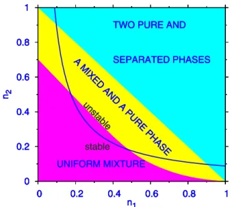
n1,1ⱕC1, C1=g12/共A1␭1/3兲. 共51兲 In this case a phase diagram showing the total densities of types 1 and 2 fermions for which the system can completely separate, can be obtained from Eq.共30兲if we allow fto vary from 0 to 1 and use conditions共50兲and共51兲. This is illus-trated in Fig. 1. The light gray area represents pure phases and the dark gray area represents the stable uniform mixture. The uniform mixture is unstable in the clear area below the curve given by inequality共14兲. For attractive interaction, one has the formation of bright solitons by modulational instabil-ity共discussed in Sec. IV兲. For repulsive interaction one can have a partially demixed configuration in the clear region in Fig.1.

Now let us see if the system spontaneously moves into the phase-separated configuration from an energetic consider-ation. The energy of the mixed system is

E_mix=S

冉

1 3A1n1

3

+n₁n₂g₁₂+1 3␭A1n2

3

冊

, 共52兲

Emix=S

冉

1 3A1n1,1

3

f3+n1,1n2,2f共1 −f兲g1,2+ 1 3A1n2,2

3

共1 −f兲3_␭

冊

.

共53兲

Equation共53兲is obtained with the use of Eq.共30兲. The en-ergy of the separated phase system with the same number of atoms is

Esep= 1

3A1S关n1,1 3 _f

+n_2,23 ␭共1 −f兲兴. 共54兲

Using Eq.共47兲, and after some straightforward algebra, the difference⌬⬅共Emix−Esep兲is given by

⌬=n_2,22 S␭1/3_共g

12−A1n2,2␭2/3兲f共1 −f兲. 共55兲 Considering the restriction共50兲 in the separated phase, Eq.

共55兲yields the following inequality:

⌬=n_2,22 f共1 −f兲S␭1/3_共

1 −n2,2/B1兲g12ⱖ0. 共56兲 For density ranges where equilibrium is possible f⫽_{0 and}

f⫽_1,Esepis always less thanEmix. Hence, energetically the two species of fermions can separate.

2. A mixed and a pure phase

Now let us consider a mixed phase共phase 1兲 and a pure phase共phase 2兲and consider the casen1,2= 0. The equality of pressure now leads to

2 3A1n1,1

3 +2

3A1␭n2,1 3

+g12n1,1n2,1= 2 3A1␭n2,2

3

. 共57兲

The equality of chemical potential of species 2 in two phases

共␮2,1=␮2,2兲 yields

n1,1=A1␭共n2,2 2

−n_2,12 兲/g12. 共58兲 Eliminating n1,1 between Eqs. 共57兲 and 共58兲 共after some straightforward algebra兲we get

2⌳共1 −x2_兲3_=x3_{− 3x+ 2, 共59兲} wherex=n2,1/n2,2,⌳=共n2,2/B1兲3. After canceling the trivial factor共1 −x兲2 _{from both sides of Eq.共59兲, we get}

2⌳共1 +x兲3_{共1 −x兲=x+ 2. 共60兲} From Eq.共60兲we find that the solutionx= 0 is obtained for ⌳= 1 corresponding to n_2,1=n_1,2= 0, n_2,2=B₁, and n_1,1=C₁. The densities of the first component are n1,2= 0 and n1,1 =C1. This is the special case considered in Sec. III B 1关see Eqs.共50兲 and共51兲兴. The solution n2,2=B1 共⌳= 1兲 is a solu-tion of two pure phases corresponding tox= 0. The domain of solution of mixed phase corresponds ton_2,2⬎B₁ 共⌳ ⬎1兲

corresponding to x⬎0 共recall that the fraction x cannot be negative兲. Hence for the present mixed phase to exist Eq.

共60兲should have the solutionx→_{+ 0 for}⌳→_{+ 1. However,}

we find from Eq.共60兲as ⌳ is made slightly greater than 1, the solution x= 0 turns negative 共unphysical兲. 关Please note 0

0.2 0.4 0.6 0.8 1

0 0.2 0.4 0.6 0.8 1

n2

n₁

0 0.2 0.4 0.6 0.8 1

0 0.2 0.4 0.6 0.8 1

n2

n₁

0 0.2 0.4 0.6 0.8 1

0 0.2 0.4 0.6 0.8 1

n2

n₁

0 0.2 0.4 0.6 0.8 1

0 0.2 0.4 0.6 0.8 1

n2

n₁

TWO PURE AND

SEPARATED PHASES UNIFORM MIXTURE

stable

unstable unstable

FIG. 1. 共Color online兲 Phase diagram for Fermi-Fermi mixture in one dimension. The plotted density n1 is in units of C1

⬅g12/共A1␭1/3兲andn2in units ofB1⬅g12/共A1␭1/3兲. The light gray

that for⌳= 1 Eq. 共60兲 has two real roots: x= 0 , 0.7399¯;

the latter共spurious兲root is not of present physical interest.兴

Hence, we conclude that a mixed and a pure phase cannot be realized in the present mixture.

Finally, one can consider the possibility of two mixed phases. The equality of pressure and chemical potential of each species in two phases leads to

2 3A1共n1,1

3

−n_1,23 兲+2

3A1␭共n2,1 3

−n_2,23 兲=g12共n1,2n2,2−n1,1n2,1兲,

共61兲

A1n1,1 2

+g12n2,1=A1n1,2 2

+g12n2,2, 共62兲

A␭n2,1 2

+g12n1,1=A␭n2,2 2

+g12n1,2. 共63兲 This set of equations have only the trivial solutions n1,1 =n1,2 and n2,1=n2,2 corresponding to uniform mixture and that is also possible when the condition of uniform mixture is satisfied. Hence, two mixed phases cannot be in equilibrium.

C. Three-dimensional mixture

From Eq.共8兲, we find that the expressions for total energy and pressure in this case are

Ej=SjEj⬅Sj

冉

3 5A3n1,j

5/3

+g12n1,jn2,j+ 3 5A3␭n2,j

5/3

冊

, 共64兲

Pj⬅− ⳵_Ej

⳵_Sj = 2 5A3n1,j

5/3

+g12n1,jn2,j+ 2 5A3␭n2,j

5/3 . 共65兲

From Eq.共22兲the chemical potentials are given by ␮1,j=A3n1,j

2/3

+g12n2,j, 共66兲

␮2,j=A3␭n2,j 2/3

+g12n1,j. 共67兲

1. Two pure phases

Again for two pure and separated phases we take n1,2 =n2,1= 0. The condition of equal pressure in two phases then leads to

n_1,15/3=␭n_2,25/3. 共68兲

The chemical potential condition␮2,2ⱕ␮2,1yields n1,1ⱖ ␭A3n2,2

2/3

/g12. 共69兲

The chemical potential condition␮1,1ⱕ␮1,2yields n2,2ⱖA3n1,1

2/3

/g12. 共70兲

Eliminatingn1,1between Eqs.共68兲and共69兲or between Eqs.

共68兲and共70兲we obtain

n2,2ⱖB3, B3=共␭2/5A3/g12兲3. 共71兲 Similarly, eliminatingn2,2between Eqs.共68兲and共69兲we get n1,1ⱖC3, C3=共␭3/5A3/g12兲3. 共72兲 In this case a phase diagram showing the total densities of type 1 and 2 fermions for which the system can completely

separate, can be obtained from Eq.共30兲if we allowfto vary from 0 to 1 and use conditions共71兲and 共72兲. This is illus-trated in Fig.2.

To see the separation of the two types of fermions from an energetic consideration, we calculate the energies of the mixed and separated configurations. The energy of the mixed phase is关23兴

Emix=S

冉

3 5A3n1

5/3

+g12n1n2+ 3 5A3␭n2

5/3

冊

, 共73兲

Emix=S

冉

3 5A3f

5/3_n 1,1 5/3

+g12n1,1n2,2f共1 −f兲

+3 5A3␭n2,2

5/3_共

1 −f兲5/3

冊

. 共74兲

The energy of the separated phase is

Esep=S

冉

3 5A3n11

5/3 f+3

5A3␭n2,2 5/3_共

1 −f兲

冊

. 共75兲

Using Eq.共68兲the difference⌬=共E_mix−E_sep兲can be written as

⌬=S兵3A3␭n2,2 5/3_f共f2/3

− 1兲/5 +g12n22 2

␭3/5f共1 −f兲

+ 3A3␭n2,2 5/3

共1 −f兲关共1 −f兲2/3

− 1兴/5其. 共76兲

Using inequality共70兲, Eq.共76兲yields

0 0.2 0.4 0.6 0.8 1

0 0.2 0.4 0.6 0.8 1

n2

n₁ 0

0.2 0.4 0.6 0.8 1

0 0.2 0.4 0.6 0.8 1

n2

n₁ 0

0.2 0.4 0.6 0.8 1

0 0.2 0.4 0.6 0.8 1

n2

n₁

TWO PURE AND

SEPARATED PHASES A

MIXED

AND

A PURE

PHASE

UNIFORM MIXTURE stable

unstable

0 0.2 0.4 0.6 0.8 1

0 0.2 0.4 0.6 0.8 1

n2

n₁

TWO PURE AND

SEPARATED PHASES A

MIXED

AND

A PURE

PHASE

UNIFORM MIXTURE stable

unstable

0 0.2 0.4 0.6 0.8 1

0 0.2 0.4 0.6 0.8 1

n2

n₁

TWO PURE AND

SEPARATED PHASES A

MIXED

AND

A PURE

PHASE

UNIFORM MIXTURE stable

unstable

FIG. 2. 共Color online兲Phase diagram for Fermi-Fermi mixture in three dimensions共3D兲. The plotted densityn1is in units ofC3

⬅共␭2/5_A

3/g12兲3andn2in units ofB3⬅共␭3/5A3/g12兲3. The light gray

⌬ ⱖA3 6

␭3

g₁₂5

冉

− 3 5f共1 −f

2/3_兲

+f共1 −f兲

−3

5共1 −f兲关1 −共1 −f兲 2/3_兴

冊

. 共77兲

For 1⬎f⬎0, the quantity given by Eq.共77兲is always posi-tive. Hence the separated phase has less energy than the mixed phase and the system will spontaneously move into the phase separated configuration. In this case also two mixed phases cannot be in equilibrium as in 1D.

2. A mixed and a pure phase

Again we consider a mixed共species 2兲and a pure共species 1兲phase and consider the casen1,2= 0. The equality of pres-sure now leads to

2 5A3n1,1

5/3

+g12n1,1n2,1+ 2 5A3␭n2,1

5/3 =2

5A3␭n2,2 5/3

. 共78兲

The equality of chemical potential of species 2 in two phases

共␮2,1=␮2,2兲 yields

n1,1=A3␭共n2,2 2/3

−n_2,12/3兲/g12. 共79兲 Eliminatingn1,1between Eqs. 共78兲and共79兲 and after some straightforward algebra we get

2⌳共1 +x兲5/3

−共1 −x兲1/3_共

3x3+ 6x2+ 4x+ 2兲= 0, 共80兲

where x=共n2,1/n2,2兲1/3 and ⌳=共n2,2/B3兲−5/9. From Eq. 共80兲 we find that the solution x= 0 is obtained for ⌳= 1 corre-sponding to n2,1= 0, n2,2=B3, n1,1=C3, n1,2= 0. This is the limiting case of two pure and separated phase studied in Sec. III C 1.关In addition for ⌳= 1, Eq. 共80兲 has the spurious or unphysical root x= 0.902 78¯, which we do not consider

here.兴 For two purely separated phases we have seen that n2,2ⱖB3 whence ⌳⬅共n2,2/B3兲−5/9ⱕ1. The domain for a mixed and a separated phase then should have⌳ ⬎1. To find this domain we solve Eq. 共80兲 for x⬎0 using different ⌳. Such solutions appear in the range 1.217¯ⱖ ⌳ ⱖ1. Using

this solution forxwe obtainn2,2andn2,1from the definitions of ⌳ and x, respectively. Finally,n1,1 is obtained from Eq.

共79兲. The results so-obtained forn_2,2,n_2,1, and n_1,1for dif-ferent⌳ are used in

n1=fn1,1 and n2=fn2,1+共1 −f兲n2,2, 共81兲 to calculate the domain of n1 and n2, by varying f in the range 1⬎f⬎0, which allows a pure and a mixed phase.

We show the 3D phase diagram for total densities of type 1 and 2 fermions in Fig.2. In this figure the light gray area represents the domain of two separated phases and the clear area that of a mixed and a separated phase as calculated above. The remaining dark gray area represents the domain of uniform mixture. The uniform mixture is unstable above the curve given by Eq. 共16兲. Qualitatively, Fig. 2 is quite similar to Fig. 3 of Viveritet al.关23兴for a Bose-Fermi mix-ture.

If we compare Figs.1and2 we find that in 1D the pure phases appear at small densities, and uniform mixture at large densities. The uniform mixture is stable at larger

den-sities. The opposite happens in 3D. If we compare the find-ings of Viveritet al.关23兴for a study of the phase diagram of a Bose-Fermi mixture in 3D and compare with the study of Das 关24兴 in 1D we find that such an inversion also takes place there. Moreover in 1D there cannot be a mixed and a pure phase for a Fermi-Fermi mixture, which is possible in 3D.

IV. DYNAMICAL EQUATIONS IN QUASI-1D SUPERFLUID FERMI-FERMI MIXTURE

A. Model

Of the three-dimensional possibilities—1D, 2D, and 3D— the 1D case deserves special attention. In 1D, if the interspe-cies Fermi-Fermi interaction is attractive, in the domain of instability of the uniform mixture one can have the formation of bright soliton by modulational instability. To perform a careful study of the nature of these bright solitons共and their dynamical stability兲we derive the Euler-Lagrange equations in 1D from its Lagrangian density.

We consider a mixture of N1 superfluid atomic fermions of massm1共=m兲andN2 superfluid atomic fermions of mass m2共=m/␭兲 at zero temperature trapped by a tight cylindri-cally symmetric harmonic potential of frequency␻_⬜in the transverse共radial cylindric兲direction. We assume factoriza-tion of the transverse degrees of freedom. This is justified in 1D confinement where, regardless of the longitudinal behav-ior or statistics, the transverse spatial profile is that of the single-particle ground state关24,54,55兴. The transverse width of the atom distribution is given by the characteristic har-monic length of the single-particle ground state: a_⬜j =

冑

ប/共m_j␻_⬜兲, with j= 1 , 2. The atoms have an effective 1D behavior at zero temperature if their chemical potentials are much smaller than the transverse energy ប␻_⬜ 关24,54,55兴. The interspecies Fermi-Fermi interaction is characterized by a contact potential with scattering length a12, which can be repulsive or attractive.

We use a mean-field Lagrangian to study the static and collective properties of the 1D superfluid Fermi-Fermi mix-ture as in the Ginzburg-Landau theory关12兴. The Lagrangian densityL of the mixture reads

L=L₁+L₂+L₁₂. 共82兲

The term L_i is the fermionic Lagrangian for component i, defined as

L_i=iប

2

冉

␺i ⴱ⳵␺i

⳵_t −␺i ⳵_␺iⴱ

⳵_t

冊

− ប2 2meff共

i兲

冏

⳵_␺i

⳵_z

冏

2

−A1 共i兲

3 兩␺i兩 6

,

共83兲

whereA₁共i兲=ប2_␲2_/共8m

Finally, the Lagrangian densityL₁₂ of the interaction be-tween the two Fermi components is taken to be of the fol-lowing standard zero-range form关33,54兴:

L_{12= −}g12兩␺1兩2兩␺2兩2, 共84兲

where g12= 2ប␻⬜a12 is the 1D Fermi-Fermi interaction strength.

The Euler-Lagrange equations of the Lagrangian L _are

the two following coupled partial differential equations:

iប⳵_t␺1=

冉

₋ ប 2

4m1 ⳵

z 2

+A₁共1兲n₁2+g12n2

冊

␺1, 共85兲

iប⳵_t␺2=

冉

₋ ប 2

4m2 ⳵

z 2

+A1共 2兲_n

2 2

+g12n1

冊

␺2, 共86兲

with the normalization兰−⬁⬁兩␺i兩2dz=Ni.

It is convenient to work in terms of dimensionless vari-ables defined in terms of a frequency ␻ and length l

⬅

冑

ប/共2m1␻兲 by ␺j=␺ˆj/

冑

l, t= 2tˆ/␻, z=zˆl, and g12=gˆ12ប2/

共4m1l兲. With these new variables Eqs.共85兲and共86兲 can be written as

i⳵_t␺1=共−⳵z 2

+An₁2+g12n2兲␺1, 共87兲

i⳵_{t␺2=共−␭}⳵ z 2

+␭An₂2+g12n1兲␺2, 共88兲 whereA⬅␲2_{/ 2 and where we have dropped the carets over} the variables, and where ␭=m1/m2, ni=兩␺i兩2, i= 1 , 2 with the normalization兰−⬁

⬁ _n

idz=Ni. Equations共87兲and共88兲with diagonal quintic nonlinearity are the equations satisfied by two coupled TG Bose gas关36兴and hence the analysis of Sec. IV also applies to a TG gas.

For stationary states the solution of Eqs. 共87兲 and 共88兲

have the form␺i=␾iexp共−i␮it兲where␮iare the respective chemical potentials. Consequently, these equations reduce to

␮1␾1=共−⳵z 2

+An₁2+g12n2兲␾1, 共89兲

␮2␾2=共−␭⳵z 2

+␭An2 2

+g12n1兲␾2. 共90兲 A repulsive interspecies Fermi-Fermi interaction is produced by a positiveg12, while an attractive Fermi-Fermi interaction corresponds to a negativeg12.

B. Modulational instability

To study analytically the modulational instability关35,56兴

of Eqs.共87兲and共88兲we consider the special case of attrac-tive Fermi-Fermi interaction while these equations reduce to

i⳵_t␺1=共−⳵ z 2

+A兩␺1兩4−g12兩␺2兩2兲␺1, 共91兲

i⳵_{t␺2=共−␭}⳵ z 2

+A␭兩␺2兩4−g12兩␺1兩2兲␺2, 共92兲 where we have taken the interspecies interaction to be attrac-tive by inserting an explicit negaattrac-tive sign ing12.

We analyze the modulational instability of a constant-amplitude solution corresponding to a uniform mixture in coupled Eqs.共91兲and共92兲by considering the solutions

␸10=Ꭽ10exp共i␦1兲 ⬅Ꭽ10eit共g12Ꭽ20

2_−A

Ꭽ₁₀4兲_{, 共93兲}

␸20=Ꭽ20exp共i␦2兲 ⬅Ꭽ20eit共g12Ꭽ10

2₋

␭AᎭ₂₀4兲_{, 共94兲}

of Eqs. 共91兲 and共92兲, respectively, whereᎭi0 is the ampli-tude and␦ia phase for componenti. The constant-amplitude solutions, describing a uniform mixture, develop an ampli-tude-dependent phase on time evolution. We consider a small perturbationᎭiexp共i␦i兲to these solutions via

␸i=共Ꭽi0+Ꭽi兲exp共i␦i兲, 共95兲

where Ꭽi=Ꭽi共z,t兲. Substituting these perturbed solutions in Eqs.共91兲and共92兲, and for small perturbations retaining only the linear terms inᎭiwe get

i⳵_tᎭ1+⳵_z2_{Ꭽ1− 2AᎭ10}4共_Ꭽ1+Ꭽ1ⴱ兲₊g₁₂Ꭽ10Ꭽ20共Ꭽ2+Ꭽ2ⴱ兲= 0,

共96兲

i⳵_tᎭ2+␭⳵ z 2

Ꭽ2− 2␭AᎭ20 4 _共

Ꭽ2+Ꭽ2ⴱ兲+g12Ꭽ10Ꭽ20共Ꭽ2+Ꭽ2ⴱ兲= 0.

共97兲

We consider the complex plane-wave perturbation

Ꭽi共z,t兲=A_i1cos共Kt−⍀z兲+iA_i2sin共Kt−⍀z兲 共98兲

with i= 1 , 2, where A_{i1 and} A_{i2 are the amplitudes for the}

real and imaginary parts, respectively, andKand⍀are fre-quency and wave numbers.

Substituting Eq.共98兲in Eqs.共96兲and共97兲and separating the real and imaginary parts we get

−A₁₁K=A₁₂⍀2

, 共99兲

−A₁₂K=A₁₁⍀2− 2g12Ꭽ10Ꭽ20A21+ 4AᎭ10 4_A

11, 共100兲 fori= 1, and

−A₂₁K=A₂₂⍀2␭, 共101兲

−A₂₂K=A₂₁⍀2_␭

− 2g12Ꭽ10Ꭽ20A11+ 4A␭Ꭽ20 4_A

21,

共102兲

fori= 2. EliminatingA_{12between Eqs.共99兲and共100兲we get}

A_11关K2−⍀2共⍀2+ 4AᎭ10 4

兲兴= − 2A₂₁g12Ꭽ10Ꭽ20⍀2,

共103兲

and eliminatingA_{22between Eqs.共101兲and共102兲we have}

A_21关K2−⍀2␭共⍀2␭+ 4A␭Ꭽ20 4 _兲兴

= − 2A₁₁g12Ꭽ10Ꭽ20⍀2␭.

共104兲

Finally, eliminatingA₁₁andA₂₁ from Eqs.共103兲and共104兲

and recalling that the density of the uniform mixturen1and n2 of the two species are given by ni=Ꭽi0

2

2K= ±⍀兵共⍀2 +⍀2_␭

+ 4An1 2

+ 4A␭2_n 2 2

兲

±关共⍀2 −⍀2_␭2

+ 4An1 2

− 4A␭2_n 2 2

兲2 + 16g12

2

␭n1n2兴1/2其1/2.

共105兲

For stability of the plane-wave perturbation,Kmust be real. For any⍀this happens for

共4An1 2

+ 4A␭2n₂2兲2

⬎共4An1 2

− 4A␭2n₂2兲2 + 16g12

2 _n 1n2␭,

共106兲

or for

4A2␭n1n2ⱖg12 2

. 共107兲

However, for 4A2␭n1n2⬍g12 2

,K can become imaginary and the plane-wave perturbation can grow exponentially with time. This is the domain of modulational instability of a constant-amplitude solution共uniform mixture兲signaling the possibility of a coupled Fermi-Fermi bright soliton to appear.

关Compare with inequality共14兲of Sec. II B describing stabil-ity of a uniform mixture. The transformation of the quantities in inequality共14兲to the dimensionless variables of inequality

共107兲can be performed with the definitions given after Eq.

共86兲.兴

C. Variational results

Here we develop a variational localized solution to Eqs.

共89兲and共90兲noting that these equations can be derived from the Lagrangian关57兴

L=

冕

−⬁

⬁ 关␮1␾1

2 +␮2␾2

2 −共␾₁

⬘兲

2

−共␾₂

⬘兲

2 −␾₁6

A/3

−␭␾₂6A/3 −g12␾1 2

␾₂2兴dz−␮1N1−␮2N2 共108兲 by demanding␦L/␦␾1=␦L/␦␾2=␦L/␦␮1=␦L/␦␮2= 0.

To develop the variational approximation we use the fol-lowing Gaussian ansatz关58兴:

␾1共z兲=␲−1/4

冑

N1␣1

w1

exp

冉

− z 2

2w1

2

冊

, 共109兲

␾2共z兲=␲−1/4

冑

N2␣2

w2

exp

冉

− z 2

2w2

2

冊

, 共110兲 where the variational parameters are␣j, the solitons’ norm, andwjwidth, in addition to␮j. The substitution of this varia-tional ansatz in Lagrangian共108兲yields

L=␮1N1共␣1− 1兲+␮2N2共␣2− 1兲− N1␣1

2w1 2 −

N2␣2

2w2 2

− A␣1 3

N₁3

3␲

冑

3w1 2−

A␭␣₂3N₂3

3

冑

3␲w₂2−

g₁₂N₁N₂␣₁␣₂

冑

␲共w1

2 +w2

2

兲. 共111兲

The first variational equations emerging from Eq. 共111兲, ⳵_L/⳵_␮1=⳵_L/⳵_{␮2= 0, yield ␣1=␣2= 1. Therefore, the} condi-tions␣1=␣2= 1 will be substituted in the subsequent varia-tional equations. The variavaria-tional equations⳵L/⳵w_j= 0 lead to

1 +2N1 2 A

3␲

冑

3+

g12N2w1 4

冑

␲共w₁2+w₂2兲3/2= 0, 共112兲

1 +2N2 2

A␭

3

冑

3␲ +

g12N1w2 4

冑

␲共w1 2

+w2 2

兲3/2= 0. 共113兲 The remaining variational equations are ⳵_L/⳵_{␣j= 0, which} yield␮as a function ofwj’s, and g’s,

␮1= 1 2w1

2+

冑

3N1

2 A

3␲w1 2 +

g12N2

冑

␲共w₁2+w₂2兲, 共114兲

␮2= 1 2w2

2+

冑

3N2

2 ␭A

3␲w₂2 +

g₁₂N₁

冑

␲共w1

2 +w2

2

兲. 共115兲

Equations 共112兲–共115兲 are the variational results which we shall use in our study of bright Fermi-Fermi solitons.

D. Numerical results

For stationary solutions we solve time-independent equa-tions共89兲and共90兲by using an imaginary time propagation method based on the finite-difference Crank-Nicholson dis-cretization scheme of time-dependent equations 共87兲 and

共88兲. The nonequilibrium dynamics from an initial stationary state is studied by solving the time-dependent equations共87兲

and共88兲with real time propagation by using as initial input the solution obtained by the imaginary time propagation method. The reason for this mixed treatment is that the imaginary time propagation method deals with real variables only and provides very accurate solution of the stationary problem at low computational cost 关59兴. In the finite-difference discretization we use space step of 0.025 and time step of 0.0005.

First we report results for stationary profiles of the local-ized Fermi-Fermi solitons formed in the presence of attrac-tive interspecies interaction 共negative g12兲. The fermions form BCS state共s兲 which satisfy a coupled nonlinear Schrödinger equation with repulsive共self-defocusing兲 quin-tic nonlinearity. Hence, fermions cannot form a bright soliton by itself. However, they can form a bright soliton in the presence of an attractive interspecies interaction关32兴induced by varying an external background magnetic field near a Fes-hbach resonance关13兴.

In Fig.3 we present the soliton profiles of the two com-ponents calculated by a direct numerical solution of Eqs.

共89兲 and 共90兲 and compare them with variational results

共112兲 and 共113兲. In general the numerical solutions have a profile distinct from a Gaussian shape of the variational ap-proximation. The numerical density profile reminds us of the square barrier. Nevertheless, the variational approximation presents a faithful average description. From Figs.3共a兲and 3共b兲we find that for a fixedN₁andN₂, as兩g₁₂兩is increased, the solitons become more compact and are better represented by the variational approximation. From Figs.3共b兲 and 3共c兲

fixed g12, as the number of atoms is reduced, the solitons become more compact.

Next we illustrate how well are the variational approxi-mations共114兲and共115兲for the chemical potential compared to the numerical results. In Fig.4 we plot the numerically obtained chemical potential forN1= 200, N2= 220, and␭= 1 for differentg12and compare with the variational result. We see that the overall agreement is good for allg12, although it is better for small兩g12兩.

After illustrating the soliton profiles in different states it is now pertinent to verify if these solitons are dynamically

stable under perturbation. To this end we consider the typical stationary soliton of Fig. 3共a兲 共obtained by the imaginary time propagation method兲 and subject it to the perturbation by setting ␾_j共z,t兲= 1.05⫻␾_j共z,t兲 and observe the resultant dynamics 共obtained by the real time propagation method兲. The resultant dynamics is illustrated in Fig.5. The solitons under this perturbation execute some oscillation, generate some noise, nevertheless propagate for as long as the

numeri-0 0.1 0.2 0.3 0.4

-8 -4 0 4 8

ni

(z)

z N1= 10

N2= 15

g12= -15

(a) 1 (num) 0 0.1 0.2 0.3 0.4

-8 -4 0 4 8

ni

(z)

z N1= 10

N2= 15

g12= -15

(a) 1 (num) 2 (num) 0 0.1 0.2 0.3 0.4

-8 -4 0 4 8

ni

(z)

z N1= 10

N2= 15

g12= -15

(a) 1 (num) 2 (num) 1 (var) 0 0.1 0.2 0.3 0.4

-8 -4 0 4 8

ni

(z)

z N1= 10

N2= 15

g12= -15

(a) 1 (num) 2 (num) 1 (var) 2 (var) 0 0.1 0.2 0.3 0.4 0.5

-4 -2 0 2 4

ni

(z)

z N1= 10

N2= 15

g12= -25

(b) 1 (num) 0 0.1 0.2 0.3 0.4 0.5

-4 -2 0 2 4

ni

(z)

z N1= 10

N2= 15

g12= -25

(b) 1 (num) 2 (num) 0 0.1 0.2 0.3 0.4 0.5

-4 -2 0 2 4

ni

(z)

z N1= 10

N2= 15

g12= -25

(b) 1 (num) 2 (num) 1 (var) 0 0.1 0.2 0.3 0.4 0.5

-4 -2 0 2 4

ni

(z)

z N1= 10

N2= 15

g12= -25

(b) 1 (num) 2 (num) 1 (var) 2 (var) 0 0.02 0.04 0.06 0.08 0.1

-20 -10 0 10 20

ni

(z)

z N₁= 100 N2= 150 g₁₂= -50

(c) 1 (num) 0 0.02 0.04 0.06 0.08 0.1

-20 -10 0 10 20

ni

(z)

z N₁= 100 N2= 150 g₁₂= -50

(c) 1 (num) 2 (num) 0 0.02 0.04 0.06 0.08 0.1

-20 -10 0 10 20

ni

(z)

z N₁= 100 N2= 150 g₁₂= -50

(c) 1 (num) 2 (num) 1 (var) 0 0.02 0.04 0.06 0.08 0.1

-20 -10 0 10 20

ni

(z)

z N₁= 100 N2= 150 g₁₂= -50

(c) 1 (num) 2 (num) 1 (var) 2 (var) 0 0.01 0.02 0.03 0.04 0.05

-50 -40 -30 -20 -10 0 10 20 30 40 50

ni

(z)

z N₁= 200 N₂= 300 g12= -50

(d) 1 (num) 0 0.01 0.02 0.03 0.04 0.05

-50 -40 -30 -20 -10 0 10 20 30 40 50

ni

(z)

z N₁= 200 N₂= 300 g12= -50

(d) 1 (num) 2 (num) 0 0.01 0.02 0.03 0.04 0.05

-50 -40 -30 -20 -10 0 10 20 30 40 50

ni

(z)

z N₁= 200 N₂= 300 g12= -50

(d) 1 (num) 2 (num) 1 (var) 0 0.01 0.02 0.03 0.04 0.05

-50 -40 -30 -20 -10 0 10 20 30 40 50

ni

(z)

z N₁= 200 N₂= 300 g12= -50

(d)

1 (num) 2 (num) 1 (var) 2 (var)

FIG. 3. 共Color online兲 Probability densities of the two fermion components from the numerical solution 共labeled “num”兲 of Eqs. 共89兲and 共90兲 关here normalized to unity: 兰−⬁

⬁

ni共z兲dz= 1兴 compared

with variational results 共labeled “var”兲 given by Eqs. 共112兲 and 共113兲 for␭= 1 and共a兲 N1= 10,N2= 15, andg12= −15,共b兲N1= 10,

N2= 15, andg12= −25,共c兲N1= 100,N2= 150, andg12= −50, and共d兲

N1= 200,N2= 300, andg12= −50.

-150 -120 -90 -60 -30 0

-50 -40 -30 -20 -10 0

µj

g₁₂ N₁= 200 N₂= 220

num, j=2 -150 -120 -90 -60 -30 0

-50 -40 -30 -20 -10 0

µj

g₁₂ N₁= 200 N₂= 220

num, j=2 var, j=2 -150 -120 -90 -60 -30 0

-50 -40 -30 -20 -10 0

µj

g₁₂ N₁= 200 N₂= 220

num, j=2 var, j=2 var, j=1 -150 -120 -90 -60 -30 0

-50 -40 -30 -20 -10 0

µj

g₁₂ N₁= 200 N₂= 220

num, j=2 var, j=2 var, j=1 num, j=1

FIG. 4. 共Color online兲Chemical potential ␮jof jth component

obtained from the numerical solution共labeled “num”兲of Eqs.共89兲 and 共90兲 and that obtained from the variational results共114兲 and 共115兲 共labeled “var”兲vs interspecies couplingg₁₂forN₁= 200,N₂ = 220, and␭= 1.

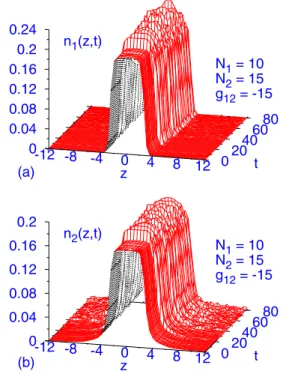
(a)

N₁= 10 N₂= 15 g₁₂= -15

-12 -8 -4 _z0 4 8 12 0 2040 6080 t 0 0.04 0.08 0.12 0.16 0.2 0.24

n₁(z,t)

(b)

N₁= 10 N₂= 15 g₁₂= -15

-12 -8 -4 _{0 4 8} 12 z 0 2040 6080 t 0 0.04 0.08 0.12 0.16 0.2

n₂(z,t)

FIG. 5. 共Color online兲Dynamics of the probability density pro-files of共a兲the first and共b兲 the second Fermi solitons of Fig.3共a兲

when att= 20 they are subject to a perturbation by setting␾j共z,t兲

= 1.05⫻␾_j共z,t兲. The solitons undergo stable propagation as long as we could continue numerical simulation. The initial soliton profile is calculated with imaginary time propagation algorithm and the dynamics studied with real time propagation algorithm. The soliton profiles are normalized to unity,兰₋⬁

⬁