Fluctuations and Fermi-Dirac Correlations in
e
+e
−-annihilation
G¨osta Gustafson
Lund University, Dept. of Theoretical Physics, S ¨olvegatan 14A, S-223 62 Lund, Sweden
Received on 6 November, 2006
In this talk I first present a short review of fluctuations ine+e−-annihilations. I then describe some new results on FD correlations. Experimental analyses ofppandΛΛcorrelations indicate a very small production radius. This result relies very strongly on comparisons with MC simulations. A study of the approximations and uncertainties in these simulations implies that it is premature to draw such a conclusion from the data.
Keywords: Fluctuations; Correlations
I. FLUCTUATIONS
In bremsstrahlung in QED, the emission of a photon does not change the current for subsequent emissions. This implies that the photon multiplicity is described by a Poisson distri-bution. As the gluons carry colour charge, the emission of a gluon in QCD changes the current relevant for the subsequent emissions. An initial hard gluon will radiate many softer glu-ons. This leads to a cascade with an exponential growth in multiplicity and to large fluctuations. The multiplicity distri-bution is approximately satisfying KNO scaling, with a width which is proportional to the average multiplicity. This short review is divided in three parts:
A. Multiplicity distribution for partons B. Effects of hadronization
C. Fractal structures
A. Multiplicity distribution for partons
In e+e−-ann. the emission of a gluon from a qq¯ pair is acoherentemission from e.g. a red and ananti-red colour charge. The result corresponds to a colour dipole with the following distribution (in the leading log approximation):
dN=α¯(k2⊥)dk
2
⊥
k2
⊥
dy, with ¯α=3αs
2π. (1)
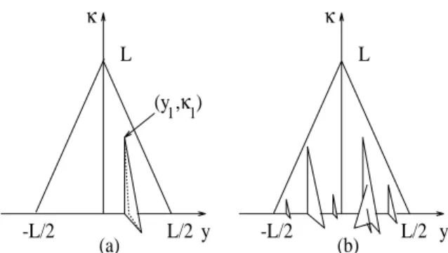
The phase space is a triangular region in(y,lnk2⊥)-space given by|y|<ln(s/k2⊥)/2, and within this triangle the density is just given by ¯α. The emission of a second (softer) gluon is given by two dipoles, one between the quark and the first gluon, and one between this gluon and the antiquark. The phase space is enlarged compared to that for the first gluon, and corresponds to the folded surface shown in Fig. 1a. For subsequent gluons the phase space is further increased, and corresponds to the fractal surface in Fig. 1b.
We letP(N,L=lns)denote the distribution in the number, N, of dipoles (which neglectingqq¯pair creation is equal to the number of gluons plus one). The Laplace transform
P
(γ,L)is given byP
(γ,L)≡∑
N
e−γNP(N,L). (2)
L L
-L/2 L/2 -L/2 L/2
(a) y (b) y
κ κ
(y
1,κ1)
FIG. 1: The phase space for gluon emission ine+e−-ann. is a tri-angular region in the(y,κ=lnk⊥2)-plane. The height of the triangle is given byL=lns. When one gluon is emitted at(y1,κ1)a second gluon with smallerk⊥can be emitted in the larger phase space shown in Fig. (a). Further softer emissions give the fractal phase space in Fig. (b).
It is then relatively easy to derive the relation (see e.g. ref. [1]) d2ln
P
dL2 = α0
L (
P
−1), where ¯α≡ α0L . (3)
Expanding eq. (2) in a Taylor series inγgives
P
=1−γhNi+1 2γ2
hN2i+. . . (4)
Inserted in eq. (3) this also implies the following equations for the average and the variance of the multiplicity distribution:
d2 dL2hNi =
α0
L hNi (5)
d2 dL2(hN
2
i − hNi2) =α0
L hN 2
i. (6)
The solutions to these equations are Bessel functions, and for high energies we get
hNi ∼L1/4exp(2pα0L) V ≡ hN2i−hNi2≈1
3hNi
2. (7)
We see that the width of the distribution is proportional to
The anomalous dimension is given by a logarithmic deriv-ative. Note that in the literature one can find different defini-tions, where the derivative is taken with respect either to lns or to lnW:
γ(0s) ≡ dlnhNi
dlns =
√
¯ α=
r 3αs
2π, (8)
γ(0W) ≡ ddlnhNi
lnW =2
√
¯ α=
r 6αs
π . (9)
I want here to add a few comments:
• hNidepends on the resolution, i.e. on the cut-off for soft emissions. It is here essential to have a cut-off which is defined locally, and not fixed in e.g. the overall cms. In the dipole cascade model this is chosen ask⊥measured in the rest frame of the emitting dipole.
• The running ofαsis important. With a constantαsthe multiplicity would grow proportional to exp(√α¯·L). i.e. much faster than the result in eq. (5).
• Non-leading corrections are very large. Terms sup-pressed by factors 1/√Lin the evolutionequationgive extra powers ofL as factors in thesolution. Also in-cluding NLL terms, the result is sensitive to effects of still higher order. For a more detailed discussion see e.g. ref. [2].
B. Hadronization effects
In string fragmentation the average hadron multiplicity,hni, in a single qq¯ system is proportional to ln(s/s0), where s0
is a scale of order 1GeV. The variance of the fluctuations,
V =hn2i − hni2, is proportional to hni, and the distribution
is thus relatively more narrow for higher energies and larger
hni. For a system of aqq¯pair and a number of gluons we get a set of string pieces with (squared) massessi,i+1= (qi+qi+1)2,
whereqiis the momentum of partoniand the partons are or-dered in colour. For the average multiplicity we then get
hni∝
∑
ln(si,i+1/s0) (10)which just corresponds to the length of the baseline of the fractal surface in Fig. 1b.
In eq. (10) the mass of a string piece should not be smaller than√s0, as it otherwise would give a negative contribution. It
is, however, also possible to define an infrared stable measure, called theλ-measure, which is insensitive to the cut-off for the perturbative cascade [3]. Simulations show that a high energy even with little gluon radiation and an event at lower energy but more radiation give equally many hadrons if they have the sameλ-value. Thus the multiplicity depends only on the mea-sureλ, which corresponds to an “effective string length”. The probability densityP(λ,L)satisfies the same evolution equa-tion (3) asP(N,L), only with different boundary conditions. This implies that the distribution inλhas the same high energy behaviour as the distribution in dipole multiplicity, eq. (5).
The fluctuations in the hadron multiplicity get contributions from both the perturbative cascade and the soft hadronization, and we get approximately
V(n,s)
hn(s)i2=
V(λ,s)
hλ(s)i2+
V(n,hλi)
hn(hλi)i2. (11)
Here the first term corresponds to the fluctuations in the cas-cade and the second one to those in the hadronization process. At high energy the first contribution dominates, while the second is larger at energies below 40-50 GeV. In ref. [3] it is shown that the total result satisfies KNO scaling with V =const· hni2, although this is not the case for any of the contributions separately below the top LEP energy. At higher energies the hadronization contribution can be neglected.
C. Fractal structures and intermittency
The baseline of the surface in Fig. 1b looks like a Koch snowflake curve. Looking at the curve with a coarser res-olution means that only emissions with k⊥>k⊥res are
in-cluded. This corresponds to cutting the surface in Fig. 1b at a higher level, corresponding to lnk2
⊥res. The length of this
curve satisfies again the same evolution equation. The bound-ary conditions are different, and with the notations L=lns andκ=lnk⊥2 the length will be proportional to the expression
Length∼L1/4κ3/4res exp(2
p
α0L−2√α0κres) (12)
It is also possible to define a (multi)fractal dimension for this curve
D=1−dlnlength
dln(κres)
=1+
rα
0 κres
=1+γ(0s) (13) (It is called a multifractal as the dimension varies with the resolutionκres.)
Fluctuations in small phase space regions, e.g. slices in rapidity∆y, can be described by the scaled moments
Cq ≡ h nqi
hniq (14)
Fq ≡ h
n(n−1). . .(n−q+1)i
hniq (15)
If the total phase space is divided inMequal pieces (which gives∆y=Y/M) a scaling behaviourFq∝Mφq is interpreted as an signal forintermittency. This can be associated with a Renyi (multifractal) dimension
Dq≡1−dq≡1− φq
q−1 (16)
In the perturbative cascade these fluctuations in small bins are dominated by the possibility to have the tip of a jet within one bin. At asymptotic energies and largeqwe then get the result [5–8]
Dq≈ q q−1
r 6αs
0 0.1 0.2 0.3 0.4
L3 data, Θ0=25 o hadrons, Q0=1.0GeV partons, Q0=1.0GeV partons, Q0=0.7GeV
ln F
2
(z)/F
2
(0)
0 0.2 0.4 0.6 0.8 1 1.2
ln F
3
(z)/F
3
(0)
0 0.5 1 1.5 2
0 0.2 0.4 0.6
z
ln F
4
(z)/F
4
(0)
0 0.5 1 1.5 2 2.5
0 0.2 0.4 0.6
z
ln F
5
(z)/F
5
(0)
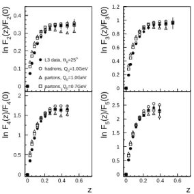
FIG. 2: L3 results for ratios of factorial moments in cones around a jet axis,Fq(z)/Fq(0), together with JETSET 7.4 PS predictions on
partonic and hadronic levels. For details see ref. [9].
L3 data, Θ0=25
o
αs=const
DLLA (a) DLLA (b) DLLA (c) MLLA
ln F
2
(z)/F
2
(0)
ln F
3
(z)/F
3
(0)
z
ln F
4
(z)/F
4
(0)
z
ln F
5
(z)/F
5
(0)
0 0.2 0.4 0.6 0.8
0 0.2 0.4 0.6 0.8 1 1.2 1.4
0 0.5 1 1.5 2 2.5
0 0.25 0.5 0.75
0 1 2 3
0 0.25 0.5 0.75
FIG. 3: Analytic QCD predictions forΛ=0.16 GeV. The curves show results forαs=const., 3 different DLL approximations and a
MLL result. For details see ref. [9].
As for the distributions in the full phase space, there are large corrections from non-leading effects and from hadronization. Therefore the analytic results have had limited success in comparisons with experimental data. As examples Figs. 2 and 3 show results from the L3 collaboration at LEP [9] for factorial moments in regions separated by cones with opening angels Θ0−Θ andΘ0+Θ around a jet axis. The
variablezis proportional to ln(Θ0/Θ). We see that although MC programs work quite well (Fig. 2), the analytic calcula-tions do not reproduce the data (Fig. 3). We note that different NLL calculations give quite different results. These calcula-tions have different approximacalcula-tions for NNLL contribucalcula-tions, which shows that the higher order corrections cannot be ne-glected. (It was early realised that BE correlations give an
important contribution to the multiplicity moments, and in the L3 analysis this effect is removed from the data.)
It is also possible to define theλ-measure for a hadronic state instead of a parton state, and it appears that analytic re-sults for theλ-measure are closer to the corresponding MC-results [6]. No comparisons with experimental data have been presented until now for such an analysis.
D. Summary
The gluon self coupling implies a fast growth of multiplic-ity and large fluctuations. In LLA we get the following as-ymptotic results:
hNi ∼ exp(2pα0lns; α0≡
3αs(Q2) 2π lnQ
2
V = 1
3hNi
2
; γ0≡ dlnhNi
dlns =
r 3αs
2π. (18) The QCD cascade has a fractal structure. The multiplicity in small phase space intervals shows intermittent features with a multifractal (Renyi) dimensionDq∼2γ(
s)
0 , and the curve
with theλ-measure has the dimension 1+γ(0s).
However, energy-momentum conservation and other non-leading effects are very important. NLL calculations give very different results if they differ at NNLL order. Hard emissions are the most important, but matrix elements factorize only for soft emissions. Therefore analytic calculations have in many cases met limited success. MC programs work, however, gen-erally quite well.
II. FERMI-DIRAC CORRELATIONS INppANDΛΛPAIRS
A. Momentum correlations
The results on baryon correlations presented here are ob-tained in collaboration with R.M. Dur´an Delgado and L. L¨onnblad [10].
Fermion correlation functions are usually fitted to the form C(Q) =N{1−λe−R2Q2}. (19) The quantityR is here interpreted as the radius of the pro-duction region for the particle pair. The different LEP exper-iments have measured momentum correlations between ΛΛ and/or ¯pp¯pairs, and obtained production radii around 0.15fm, which is much smaller than the proton radius [11–14].
In experiments the correlation functionC(Q)is determined by comparing the observed number of pairs,N(Q), with a ref-erence sample,Nref(Q):
C(Q) = N(Q) Nref(Q)
. (20)
• MC generation. This is model dependent.
• Mixed events. The event structure is changed by gluon emission, which makes it difficult to construct a sample of events with similar structure.
A common method to reduce the problems is to take adouble ratio:
C(Q) = N(Q) Nmix(Q)
Á MC(Q)
MCmix(Q)
. (21)
Here the sample of Monte Carlo events, MC(Q), should be generated without including FD correlations in the model. It is argued that the effect of different event types should be similar in the real data and the MC events, and therefore be reduced in the ratio.
The mixed pairs depend only on inclusive spectra, and the MC programs are tuned to reproduce the inclusive spectra with good precision. This implies that the tuning also gives
Nmix(Q)≈MCmix(Q) (22)
which implies that
C(Q)≈ N(Q)
MC(Q). (23)
Consequently the resultdepends very critically on a realistic MC, also if the double ratio is used in the analysis.
In the Lund string hadronization model the colour string normally breaks byqq¯pair production. The ordering of the hadrons along the string, the rank ordering, agrees on average with the ordering in rapidity, with an average separation,∆y, of the order of half a unit in rapidity. A baryon-antibaryon pair can be produced when a breakup is generated by a diquark-antidiquark pair, with quark-antiquark pairs on either side. In this picture two baryons must always be separated by at least one antibaryon (and normally also with one or more mesons). This will give a strong anti-correlation between two baryons in rapidity and in momentum. This is seen in Fig. 4, which shows correlations in pp andpp¯pairs. We see that there is a positive correlation between protons and antiprotons, which are neighbours in rank, but a negative correlation between two protons.
In the model there is also a correlation between momen-tum and space coordinates for the produced hadrons. Thus two identical baryons are (in the model) well separated also in coordinate space, and we would from this picture expect Fermi-Dirac correlations to correspond to a radius∼2−3 fm. We see that the range for theppcorrelation in Fig. 4 is given byQ∼1.5GeV∼1/(0.15fm). We note that this corresponds exactly to the correlation length reported in the experiments, although in this model the production radius is very much larger. The strength of the correlation is, however, smaller in the MC than in the data.
This raises the question: Is the difference between data and MC really a FD effect, or could the MC underestimate the strength of the correlation?
There are a number of sources for uncertainty in the MC:
0 0.5 1 1.5 2 2.5 3 3.5 4
0 1 2 3 4 5 6 7 8 9 10
Q (GeV) Correlations
proton-antiproton proton-proton antiproton-antiproton
FIG. 4: MC results for the ratioCMC(Q) =MC(Q)/MCmix(Q)for
pp- (×) andpp¯-pairs (+).
0.4 0.5 0.6 0.7 0.8 0.9 1 1.1 1.2 1.3
0 1 2 3 4 5 6 7 8 9 10
Q (GeV) MC proton correlations
a=0.1 b=0.45 GeV-2
a=0.3 b=0.58 GeV-2
a=0.354 b=0.523 GeV-2 a=0.5 b=0.7 GeV-2 a=1 b=1 GeV-2 a=2 b=2 GeV-2
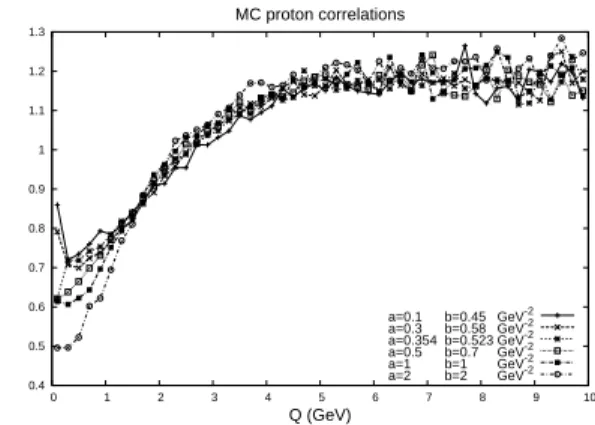
FIG. 5: The ratioCMC(Q) =MC(Q)/MCmix(Q)for different val-ues of the parametersaandb. Larger(a,b)-values give a stronger correlation and a deeper dip for smallQ.
1) There are two fundamental parameters,aandb, in the Lund model “splitting function”
f(z)∝(−z)ae−bm2/z (24) The hadron multiplicity depends essentially on the ratio(a+ 1)/b, This ratio is therefore well determined by experiments, buta andb separately are more uncertain. Small values of a andb correspond to a wide distribution f(z), and a wide distribution in the separation,∆y, between hadrons which are neighbours in rank. Large values ofaandbimply a narrow ∆y- distribution and therefore lower probability for two parti-cles to be close in momentum space. The effect of varyinga andbkeeping the multiplicity unchanged is shown in Fig. 5.
2) The parameterbis a universal constant, butamay be dif-ferent for baryons, although data are well fitted by a universal a-value. This gives some extra uncertainty.
0.2 0.4 0.6 0.8 1 1.2 1.4 1.6 1.8
0 1 2 3 4 5 6 7 8 9 10
CMC
(Q)
Q (GeV)
10000 GeV, shower off
Lund model; a=0.3, b=0.58 GeV-2
Independent fragmentation, pz> 2 GEV; a=0.5, b=0.7 GeV-2
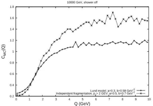
FIG. 6: A single jetwithouta junction has a large dip inCMC(Q) =
MC(Q)/MCmix(Q)for smallQ(×). This correlation is reduced by the approximate treatment in the MC of the small mass systems close to the ”junction” (+).
0.6 0.7 0.8 0.9 1 1.1 1.2 1.3
0 1 2 3 4 5 6 7 8 9 10
CMC
(Q)
Q (GeV)
91 GeV
100% protons 85% protons, 15% pions
FIG. 7: CMC(Q) =MC(Q)/MCmix(Q)with (+) and without (×) a 15% admixture of pions.
works well for inclusive distributions, but implies that the cor-relations do not correspond to the model prediction for parti-cles close to the “junction”. Fig. 6 shows results for a single jet without a junction compared with the standard result.
4) Gluon emissions imply that straight string pieces are small compared to the mass of aBBB¯ system. This gives also
extra uncertainty.
5) Pion correlations are not perfectly reproduced by the MC. As an example the DELPHI antiproton sample contains 15% pions. Fig. 7 shows results with and without a 15% pion admixture. We see that an error in the simulation of the pion-pion or pion-proton correlations also affects the esti-mated proton-proton correlations.
In summary we see that there are many effects which make the MC predictions forpporΛΛcorrelations quite uncertain. As the experimental determination of the correlations rely so strongly on a correct MC, it is therfore at present premature to conclude that the production radius has the very small value around 0.15fm.
B. Spin-spin correlations
Λparticles reveal their spin in the orientation of their decay products. This has been used to studyΛΛcorrelations without the need for a comparison with MC results. AΛΛpair with total spin 1 must have an antisymmetric spacial wave function and is therefore expected to show a suppression for small rel-ative momentaQ.ΛΛpairs with total spin 0 has a symmetric spacial wave function, and should therefore show an enhance-ment for smallQ, similar to the correlation for bosons. There-fore one expects pairs with smallQ-values to be dominantly S=0. Analyses at LEP [11, 15, 16] do indicate such an ef-fect. They are however based on rather low statistics, and the errors are presently too large for any definite conclusion about the strength and range of the effect.
C. Summary
A production radiusR∼0.15fm for baryon pairs is not con-sistent with the conventional picture of string fragmentation.
Experimental results for pp andΛΛ correlations depend sensitively on a reliable MC.
The observed (anti-)correlation has the same range inQas the correlation in the MC, but is stronger.
Uncertainties in the MC implementation are large.
Conclusion: It is therefore premature to claim evidence for a new production mechanism.
[1] B. Andersson, P. Dahlqvist, and G. Gustafson, Phys. Lett. B 214, 604 (1988).
[2] G. Gustafson and M. Olsson, Nucl. Phys. B406, 293 (1993). [3] B. Andersson, P. Dahlqvist, and G. Gustafson, Z. Phys. C44,
455 (1989).
[4] B. Andersson, G. Gustafson, and B. S¨oderberg, Nucl. Phys. B 264, 29 (1986).
[5] P. Dahlqvist, B. Andersson, and G. Gustafson, Nucl. Phys. B 328, 76 (1989).
[6] G. Gustafson and A. Nilsson, Z. Phys. C52, 533 (1991). [7] W. Ochs and J. Wosiek, Phys. Lett. B289, 159 (1992). [8] W. Ochs and J. Wosiek, Phys. Lett. B305, 144 (1993). [9] W. Kittel, S.V. Chekanov, D.J. Mangeol, and W.J. Metzger,
Nucl. Phys. Proc. Suppl.71, 90 (1999); hep-ex/9712003. [10] R.M. Dur´an Delgado, Diploma thesis,Lund preprint LU TP
06-17 (2006), and R.M. Dur´an Delgado, G. Gustafson, and L. L¨onnblad, in preparation.
[11] R. Barate et al. (ALEPH Coll.), Phys. Lett. B475, 395 (2000). [12] OPAL Coll., CERN-EP/2001, OPAL-PN486 (2001).
[13] R. Barate et al., (ALEPH Coll.), Phys. Lett. B611, 66 (2005). [14] DELPHI Coll., DELPHI 2004-038 CONF-713 (23 June, 2004),
DELPHI 2005-010 CONF-730 (30 May, 2005).
[15] G. Alexander et al. (OPAL Coll.), Phys. Lett. B384, 377 (1996). [16] T. Lesiak and H. Palka (DELPHI Coll.), CERN-EP/98-114,