www.nonlin-processes-geophys.net/22/173/2015/ doi:10.5194/npg-22-173-2015
© Author(s) 2015. CC Attribution 3.0 License.
Equilibrium temperature distribution and
Hadley circulation in an axisymmetric model
N. Tartaglione
School of Science and Technology, University of Camerino, Camerino, Italy
Correspondence to:N. Tartaglione ([email protected])
Received: 5 October 2014 – Published in Nonlin. Processes Geophys. Discuss.: 3 November 2014 Revised: 8 January 2015 – Accepted: 20 February 2015 – Published: 16 March 2015
Abstract.The impact of the equilibrium temperature distri-bution, θE, on the Hadley circulation simulated by an
ax-isymmetric model is studied. TheθEdistributions that drive
the model are modulated here by two parameters, nandk, the former controlling the horizontal broadness and the lat-ter controlling the vertical stratification ofθE. In the present
study, variations in theθEdistribution mimic changes in the
energy input of the atmospheric system, leaving as almost in-variant the Equator–polesθEdifference. Both equinoctial and
time-dependent Hadley circulations are simulated and the re-sults compared. The rere-sults give evidence that concentrated θE distributions enhance the meridional circulation and jet
wind speed intensities, even with a lower energy input. The meridional circulation and the subtropical jet stream widths are controlled by the broadness of horizontalθE rather than
by the vertical stratification, which is important only when θEdistribution is concentrated at the Equator. The jet stream
position does not show any dependence withnandk, except when the θE distribution is very wide (n =3) and, in such
a case, the jet is located at the mid-latitudes and the model temperature clamps to forcingθE. Usingn=2 andk=1, we
have the formulation of the potential temperature adopted in the classical literature. A comparison with other works is per-formed, and our results show that the model running in differ-ent configurations (equinoctial, solstitial and time dependdiffer-ent) yields results similar to one another.
1 Introduction
The Earth’s atmosphere is driven by differential heating of the Earth’s surface. At the Equator, where the heating is larger than that at other latitudes, air rises and diverges
pole-ward in the upper troposphere, descending more or less at 30◦
latitude. This meridional circulation is known as the Hadley cell. Two subtropical jets at the poleward edges of the Hadley cell form because of the Earth’s rotation and the conserva-tion of the angular momentum. A poleward shift (Fu and Lin, 2011) and an enhanced wind speed of these jets (Strong and Davis, 2007) are associated with possible Hadley cell widen-ing and strengthenwiden-ing, which has been observed in the last decades (Fu et al., 2006; Hu and Fu, 2007; Seidel et al., 2008; Johanson and Fu, 2009; Nguyen et al., 2013).
There are a few studies suggesting possible causes of these phenomena. One of the theories postulates global warming as a possible cause of Hadley cell widening (Lu et al., 2009). However, the atmosphere is a complex system containing many subsystems interacting with one another, and global warming might not be the only cause that is suggested to ex-plain the widening. Ozone depletion (Lu et al., 2009; Polvani et al., 2011), SST warming (Chen et al., 2013; Staten et al., 2011) and aerosol (Allen et al., 2012) have also been invoked to explain the Hadley cell widening.
Climate models vary to some extent in their response and the relationship between global warming and the Hadley cell is not straightforward. For instance, Lu et al. (2007) found a smaller widening than the observed one. Gitelman et al. (1997) showed that the meridional temperature gradient decreases with increasing global mean temperature, and the same result can be found in recent modeling studies (Schaller et al., 2013).
Hadley circulation. How much temperature change impacts the real Hadley circulation is not clear yet, perhaps because of discrepancies between observations, reanalysis (Waliser et al., 1999) and climate model outputs, although these differ-ences are becoming less marked because of newer observa-tional data sets or corrections of the older ones (Sherwood et al., 2008; Titchner et al., 2008; Santer et al., 2008). Hence, it is critical to understand the possible mechanisms behind the cell expansion starting from a simple model.
The objective of this study is to analyze the sensitivity of a model of symmetric circulation to the radiative–convective equilibrium temperature distribution. Our point of departure is the symmetric model used by Cessi (1998), which is a bi-dimensional model considering atmosphere as a thin spher-ical shell. This model will be briefly described in Sect. 2. The model mainly describes a tropical atmosphere; hence, it does not allow for eddies. Although eddies may play a central role in controlling the strength and width of the Hadley cell (e.g., Kim and Lee, 2001; Walker and Schneider, 2006), a symmetric circulation, driven by latitudinal differential heat-ing, can exist even without eddies, and it is a robust fea-ture of the atmospheric system (Dima and Wallace, 2003). The temperature distributions used in this study represent some paradigms of tropical atmospheres. Among the possi-ble causes that can change temperature distributions are El Niño, global warming and changes in solar activity. We will show, in Sect. 3, that the energy input is not as important as the forcing distribution. Our results are consistent with those obtained both by Hou and Lindzen (1992) (hereafter HL92) and recently by Tandon et al. (2013), who performed exper-iments similar to those described here. The conclusions will be drawn in Sect. 4.
2 The model
The model used in this study is a bi-dimensional model of the axisymmetric atmospheric circulation described in Cessi (1998). The horizontal coordinate is defined as y=asinφ, from which we have
c(y)=cosφ= q
1−y2/a2
, (1)
whereais the radius of a planet having a rotation rate; the height of the atmosphere is prescribed to beH.
The model is similar to the Held and Hou model (HH80), but it prescribes a horizontal viscosityνHother than the
verti-cal viscosityνv. The prognostic variables are the angular
mo-mentumM, defined asM= a c2+u c, whereurepresents the zonal velocity; the zonal vorticityψzzwith the meridional
stream functionψis defined by ∂yψ≡w,
∂zψ≡ −cv, (2)
and the potential temperature θ that is forced towards a radiative–convective equilibrium temperature θE. Starting
from the dimensional equations of the angular momentum, zonal vorticity and potential temperature, we will obtain a set of dimensionless equations. The new equations are non-dimensionalized using a scaling that follows Schneider and Lindzen (1977), but the zonal velocityuis scaled with a. A detailed description can be found in Cessi (1998).
The non-dimensional model equations are
Mt=
1 R
(
Mzz+µ
c4c−2M
y
y
)
−J (ψ, M), (3a)
ψzzt =
1 R2E2yc
−2M2
z−
1 c−2J
ψ, c−2ψzz
+ 1
RE2c−2θy+ 1 Rc−2
h
c−2ψzzzz+µψzzyy
i ,
(3b) θt=
1 R
θzz+µ
h c2θy
i
y+α
θE(y, z)−θ
−J (ψ, θ ). (3c) The termJ (A, B)=AyBz−AzByis the Jacobian.
The thermal Rossby numberR, the Ekman numberE, the ratio of the horizontal to the vertical viscosityµand the pa-rameterαare defined as
R≡gH 1H/
2a2; E≡νV/
H2;
µ≡
H2/a2νH/νV;α≡H2/ (τ νV) . (4)
The termαis the ratio of the viscous timescale across the depth of the model atmosphere to the relaxation timeτ to-ward the radiative–convective equilibrium.
The boundary conditions for the set of Eq. (3) are Mz=γ
M−c2, ψzz=γ ψz,
ψ=θz=0 atz=0,
Mz=ψzz=ψ=θz=0 atz=1, (5)
whereγ=C Hν
V is the ratio of the spin-down time due to the drag to the viscous timescale; the bottom drag relaxes the angular momentum M to the local planetary value a c2 through a drag coefficientC.
The model flow started from an isothermal state at rest and is maintained by a Newton heating function where the heating rate is proportional to the difference between the model potential temperature and a specified radiative– convective equilibrium temperature distribution, which fol-lows the HH80 one:
θE=
4 3−y
2+1V
1H
z−1
2
. (6)
by Eq. (6). HH80 suggested that the impact of latent heat released by water vapor condensation can be incorporated into dry axisymmetric models by modifying the meridional distribution of θE. HL92 followed the HH80 argument and
altered the concentration ofθEunder the constraint of equal
energy input. The resulting θE distributions used by HL92
were peaked distributions on and off the Equator, resulting in a stronger Hadley circulation with respect to the circula-tion obtained by applying Eq. (6). Tandon et al. (2013) used narrow and wide thermal forcing to mimic El Niño or global warming effects on a tropical circulation in a global circu-lation model. On the opposite side, in fact, we can suppose that, if a warmer climate happens, especially in the tropical regions, a very weak gradient of the equilibrium temperature θE will have a greater extent in latitude, expanding
conse-quently the tropical region. This has already occurred in the past, especially in the middle Cretaceous and Eocene, when the tropics extended up to 60◦. This is the so-called equable
climate (e.g., Greenwood and Wing, 1995) where roughly equal temperatures are present throughout the world. During those geological ages, the temperature was generally higher everywhere, but adding a constant to the temperature does not change the response of this kind of model. The Equator– pole temperature gradient was smaller than the present situ-ation, whereas we prescribe a constant surface Equator–pole θEgradient. As we shall show afterwards, this is necessary to
demonstrate that it is the tropical temperature gradient that drives the Hadley circulation. Thus, in order to study sys-tematically these different conditions, we adopt the strategy to build forcing functions dependent on a parameter that con-trols theθEgradient in the tropical regions. Since, with
dif-ferent horizontal distributions ofθE, we can figure out that,
even the vertical distribution could be affected by some phys-ical mechanisms that make the atmosphere more or less sta-ble than the stratification described by the zcomponent of Eq. (6). The meridional and vertical changes of equilibrium temperature can be obtained by changing the exponents ofy andzin Eq. (6), transforming Eq. (6) in the following equa-tion:
θE=
4 3− |y|
n+1V
1H
zk−1
2
. (7)
The termsnandk control the horizontal distribution ofθE
and its stratification, respectively. Small values ofnare asso-ciated with concentratedθEdistributions. Increasingnmeans
increasing the broadness of the θE distribution. Values ofk
larger than 1 mean more stable stratification at upper levels; vice versa, smallerkvalues mean that lower levels are more stable than upper levels. Thus, it becomes quite natural to explore the response of the Hadley circulation by changing the parametersnandk, which control the distribution ofθE,
in the closest ranges of 2 and 1, respectively. Thus,nandk will change from 0.5 to 3 with a 0.5 step, in such a way as to have a set of 36 simulations. Whenn=2 andk=1, Eq. (7) becomes Eq. (6), and the experiment performed with such
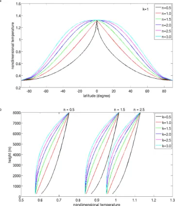
Figure 1. Vertical (a) and meridional (b) average of non-dimensional equilibrium temperature as a function of n with k=1 (a)andkwithn=0.5, 1 and 1.5(b). Dimensional values are obtained by multiplying byθ0=300 K.
values ofn andk will be considered the reference experi-ment.
The meridional and vertical averages ofθEare shown in
Fig. 1. Heating functions with annvalue equal to 0.5 should not be regarded as unreal, but merely as a simple way of rep-resenting a specific state of the atmosphere. The same asser-tion is valid for all other parameters. Asnincreases, the av-erage temperature increases as well, but the meridional gra-dient decreases in the tropical regions (Fig. 1a).
With the prescribedθEas specified by Eq. (7),θEvalues at
the boundaries and its Equator–pole difference temperature remain invariant with respect ton, for a givenkvalue. The energy input is not constant here, which differs from HL92, which analyzed the influence of concentration heating per-turbing the forcing functionθE(y, z)in such a way thatθE
av-eraged over the domain remained constant. It is easily visible in Fig. 1b. Highernvalues, keepingkinvariant, have higher averagedθEat all levels. The same is true fork, with higher
k values, forn constant; θE at each level is always higher
than that with lowerk values. The Equator–poleθE
differ-ences at upper and lower vertical boundaries are the same for all the experiments having the samek; the vertical averaged θEchanges as a function ofk, fornconstant.
paper. One can expect that global warming will broaden the temperature distribution, but, at the same time, it could have an impact above all on the sea surface temperature (SST), bringing more water in the upper atmosphere, which changes the vertical distribution, especially of the temperature in the intertropical convergence zone (ITCZ). It is supposed that, in first approximation, oceans force the atmosphere, so we have to allow for the possibility that increasing SST can change the forcing distribution. Increasing uniformly SST the Hadley cell might show a poleward expansion, as showed by Chen et al. (2013) by an aqua-planet model, but in that case, the mechanism was supposed to be related mainly to mid-latitude eddies rather than a tropical forcing. Since other causes can change the temperature distribution of a planet, such as changes in the solar activity for instance, we will fo-cus on the temperature distribution regardless of its cause.
In this model, the atmosphere is dry, as in many other studies (e.g., Schneider, 1977, HH80, Caballero et al., 2008); changing theθEdistribution allows for a change in the static
stability. Looking at the averageθEalong the vertical
direc-tion, low values ofkare related to low values of static stabil-ity, especially at higher levels of the model atmosphere.
The Brunt–Väisälä frequency, when the atmosphere reaches the equilibrium, will be
N2= gk1V/1Hz
(k−1)
4/3−yn+1
V/1H zk−1/2
. (8)
It is clear from Eq. (8) that the Brunt–Väisälä frequency does not depend onnat the poles and Equator. On the contrary, it depends on k; large values of kimply a more stable atmo-sphere in the upper levels, especially at the poles, making the model atmosphere more similar to the real one, simulat-ing in some respects a sort of tropopause. Moreover, this is equivalent to creating a “physical” sponge layer in the upper levels of the model that will have some effects on the vertical location of the stream function maximum.
Starting from Eq. (7), a set of experiments were performed changingnandkin such a way as to have a set of numerical results. In order to isolate the contribution of the θE
distri-bution to the solution of Eq. (3), a set of parameters will be used:
a=6.4×10⁶m =2π/8.64×104s−1 1H=1/3 1V=1/8
g=9.8 m s−2 C=0.005 m s−1 H=8×10³m τ=20 days
νV=5 m2s−1 νH=1.86 m2s−1. (9)
The parameters in Eq. (9) are the same as those used by Cessi (1998).
n
k
maximum stream function
0.5 1 1.5 2 2.5 3 0.5
1 1.5 2 2.5 3
2 4 6 8 10 12 14 16 18
a
n
k
maximum zonal wind speed
0.5 1 1.5 2 2.5 3
0.5 1 1.5 2 2.5 3
40 50 60 70 80 90
b
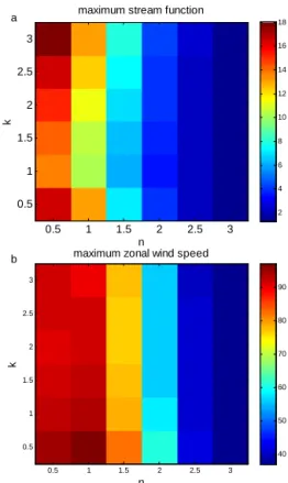
Figure 2.Maximum non-dimensional stream function(a)and zonal wind speed (m s−1)(b) as a function of parameters n andk for the steady solution. Dimensional values of the stream function are obtained by multiplying byνVR ε−1=484 m2s−1.
3 Numerical results
This section is divided into three subsections, the first show-ing the results of the model applyshow-ing the equinoctial con-dition, when the Sun is assumed to be over the Equator. The solution is steady, as already shown for instance in Cessi (1998). The second subsection will show the results of the model having aθEdistribution described by Eq. (7) but
moving following a seasonal cycle. Finally, the casen=2 andk=1 will be discussed in the third subsection in com-parison with previous studies.
3.1 Equinoctial simulations
The absolute value of the maximum stream function in-tensity under the equilibrium conditions for the 36 experi-ments is shown in Fig. 2. Whenn=0.5, withkconstant, the circulation is always the strongest. The stream function in-tensity is inversely proportional ton(Fig. 2a). Withn=0.5, the experiment resembles the one described in HL92, where they concentrated the latitudinal extent of heating, and this led to a more intense circulation. However, they imposed the forcing functionθE(x, y)in such a way that its average
over the domain remained the same as in the control exper-iment, i.e., without changing the energy input. They found that concentration of the heating through a redistribution of heat within the Hadley cell led to a more intense circula-tion without altering its meridional extent. Instead, here, it is evident from Fig. 1 that the experiment with n=0.5 has an energy input lower than the other cases. Nevertheless, the Hadley circulation is always more intense than the other cases and opposite to highernvalue experiment results; the circulation is confined closer to the Equator. Thus, the results of HL92 are extended to a more general case with a lower en-ergy input. It is worth noticing that the constraint of an equal Equator–pole gradient of meanθEis assumed here differently
from HL92 (Fig. 1a).
The dependence onkis not as straightforward as the one onn, instead. The stream function reaches the highest value for n=0.5 and k=3. With highn values, the Hadley cell strength is lower, and the dependence onk loses its impor-tance. In other words, in our model, the symmetric circula-tion strength is modulated byk only when the equilibrium temperature distribution is concentrated on the Equator.
Figure 2b shows the maximum zonal wind speed as a func-tion of nandk, it is inversely proportional ton, the depen-dence onkis not as clear as the one onnand, whenn=3, it almost vanishes in accordance with the behavior of the max-imum stream function. These results are in agreement with HL92, who found a stronger zonal wind when the forcing was concentrated at the Equator.
Some observational studies define the border of the Hadley cell where the stream function goes to 0 at 500 hPa (e.g., Frierson et al., 2007). Since, in our model, the zero stream function is at the poles, it is problematic to define an edge of the Hadley cell based on the zero stream function. Moreover, circulation intensity changes greatly in our exper-iments, so it is puzzling to define an edge of the Hadley cell based on an absolute value of the circulation itself. Hence, we will look at the location of the maximum stream func-tion, and we will analyze its poleward shift as a function of the two parametersnandk. The edge of the cell might also be defined by values of isolines that are relative with respect to the maximum value, for example 1/4 of the stream function. For the sake of clarity, this definition would be an operational one, and does not follow the definition used in observational studies, for example by Dima and Wallace (2003) or Frierson et al. (2007).
n
k
latitude of the maximum streamfunction value
0.5 1 1.5 2 2.5 3
0.5 1 1.5 2 2.5 3
6 8 10 12 14 16 18
a
n
k
height of the maximum streamfunction value
0.5 1 1.5 2 2.5 3
0.5 1 1.5 2 2.5 3
1500 2000 2500 3000 3500 4000 4500 5000 5500 6000
b
Figure 3.Latitude (degrees)(a)and height (m)(b)of the maximum non-dimensional stream function as a function of parametersnand k.
The latitude of the maximum stream function value shows a general dependence onn andk. It increases with n and decreases withk. However, as shown in Fig. 3a, this depen-dence is not straightforward or linear, although we have a few exceptions, for instance whenk=n=0.5. Hence, in general, whennincreases, and the temperature gradient in the trop-ics decreases, even though the total energy input is larger, the stream function is weaker and the Hadley cell moves poleward. This result is in agreement with other model out-comes (Frierson et al., 2007; Lu et al., 2008; Gastineau et al., 2008; Tandon et al., 2013). The model predicts a weaken-ing of circulation, in contrast to the strengthenweaken-ing, together with widening of the Hadley circulation for the past three decades observed by Liu et al. (2012) and Hu and Fu (2007). However, Liu et al. (2012) showed that if the observations start from 1870, the Hadley cell has become more narrow and stronger.
The height of the maximum stream function value is con-fined for almost all the simulations to under 2200 m and the general rule is that, whennincreases, the height of the maximum decreases; however, a few experiments, those with k=0.5 andn=0.5, 1 and 1.5, have the maximum value be-tween 4300 and 5600 m (Fig. 3b).
Table 1.Latitudes (in degrees) of the maximum wind speed for the equinoctial and time-dependent solutions whenk=1 as a function of the parametern.
n 0.5 1 1.5 2 2.5 3
Equinoctial 27.4 28.7 27.4 26.1 28.7 47.7
Time dependent 28.7 28.7 28.7 27.4 27.4 44.4
andk. It is always confined between 26 and 29◦off the Equa-tor; however, when n=3, there is an abrupt transition to about 48◦, independently of thekvalue. In Table 1, we show the latitude of the maximum wind speed whenk=1 for dif-ferentnvalues.
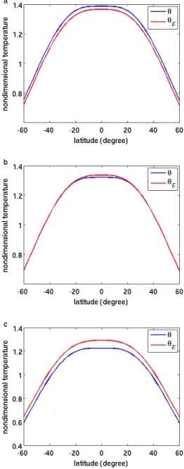
The difference betweenθEandθ, once the model reaches
the equilibrium, is quite interesting when k is not equal to 1. Figure 4 shows meridional distributions ofθE andθ for
n=3 and k=0.5, 1 and 3. In Fig. 4a, k=0.5, and θE is
under θ; whenk=1, we find that θE is over θ in a region
around the Equator (Fig. 4b), withθEcrossingθat about 47◦,
finding again the equal area condition suggested by HH80, and that explains approximately the jet location, whereas in Fig. 4c, withk=3, we can see howθEis overθ.
Neverthe-less, all simulations with n=3 give almost the same solu-tion, in terms of circulation strength and jet location (Figs. 2 and 3). For other values ofn, the results are similar, but the differences betweenθEandθare not so visible.
We can understand these findings in the light of Cessi (1998), who analyzed the model described by the set of Eq. (3) by using an asymptotic expansion of the variables M,θ andψ in power series of the Rossby numberR. The meridional advection, in the nonlinear term of the expan-sion, depends on the differences betweenθEandθ,θE−θ; on
the cube of the meridional temperature gradient; and quasi-linearly on the imposed stratification. Deducing that for un-stable stratification, this term would appear as a negative dif-fusivity term, a condition that can exist even with some sta-ble stratifications (Cessi, 1998). This seems to be our case whenk=0.5. Although the stratification imposed by Eq. (7) is stable, i.e.,∂θE
∂z >0, the second derivative is negative when
k=0.5, reducing the stability at upper levels, so this situation can be seen as a way of simulating the effect of the latent heat released by water vapor condensation. Running the model with an enhanced vertical viscosity (5 times the value de-fined in Eq. 9), the situation described by Fig. 4a changes to look like that of Fig. 4b. Defining stratification withk=0.5 is consequently equivalent to reducing the actual vertical dif-fusivity.
Whenk=3, the air in upper levels is very stable, and the upward flow has to do more work to rise at upper levels; most of the thermal energy that drives the model atmosphere is evidently dissipated by this work, reducing the actual en-ergy with respect to that provided byθE. We performed some
runs with reduced vertical viscosity; the actual value ofθin Fig. 4c slightly increases, becoming closer to θE, but it
re-Figure 4.Vertically averagedθ (blue line) and θE (red line) for
the simulations withn=3 andk=0.5(a),k=1(b)andk=3(c). Dimensional values are obtained by multiplying byθ0=300 K.
mains constant under theθEcurve, even for values of
verti-cal viscosity close to 0.1 (with vertiverti-cal viscosity very close to 0 or negative, the model blows up). This should not be interpreted as an unphysical result, but it has to be seen as the difficulty of flow temperature in relaxing toθE because
of very stable imposed stratification. In any case, the Hadley circulation is still reproduced, demonstrating the robustness of the model.
Withngetting larger, theθE distribution becomes flatter
in the tropical region andθclamps toθE. In general, we
is equivalent to a weakening of the rotation (Cessi, 1998). If the circulation is proportional to the cube of the meridional temperature gradient, it is quite evident that, when such a gra-dient has high values in the tropical region, the circulation is vigorously driven by this term, whereas, when it approaches zero, it is the term θE−θthat dominates. HH80 found that
the edge of the Hadley cell was at the mid-latitudes when the planetary rotation was lower than that of the Earth. Since this phenomenon is observed here for a wider forcing distribu-tion, this common result may be attributed to the process of homogenization of momentum and temperature in the equa-torial region.
In order to explain equable climates like those supposed to have occurred in the Cretaceous and Eocene, Farrell (1990) formulated an axisymmetric model starting from that of Held and Hou and used a forcing withn=2 andk=1, introducing a radiative–diffusive term to make flatter the model tempera-ture gradients in the tropics. For high values ofn, theθ distri-butions are similar to those obtained by Farrell (1990), with high values of its diffusive parameter. In some respects, flat-tening of the forcing distribution is equivalent to having a dif-fusive term, and this also explains Fig. 4c. The Farrell (1990) model showed a poleward shift of the zonal jet, and it has to be noticed that a poleward shift of the subtropical jets was also observed by HH80 when increasing the vertical viscos-ity.
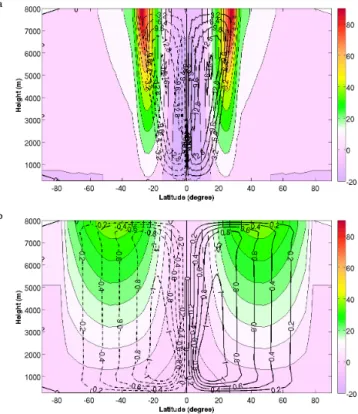
Figure 5 shows the stream function and the zonal wind speed for the experimentsn=k=0.5 (Fig. 5a) andn=k=3 (Fig. 5b). The parameter ncontrols the Hadley cell and jet stream widths. The results show that, with n=k=0.5, the Hadley cell and jet streams are quite narrow. As far as the vertical position of the maximum value of the stream func-tion is concerned, experiments withk=0.5, 1 and 1.5 exhibit particular behavior with respect to the other experiments. The stream function has its maximum at upper levels. This is re-lated to the different stratification imposed by the parame-terk. Stratification with low values ofkfavor air to move to higher levels with respect to experiments with higherk val-ues.
3.2 Time-dependent simulations
Since heating depends on solar irradiation, it is of interest to analyze the solutions obtained by the annually periodic thermal forcing and to compare it with the steady solutions described previously in this paper. Starting from Eq. (7), we can formulate an equilibrium temperature distribution having the maximum heating off the Equator at latitudey0:
θE=
4
3− |y−y0|
n+1V
1H
zk−1
2
, (10)
wherey0in Eq. (10) is dependent on time according to
y0(t )=sin
ϕ0π 180
·sin
2π t 360 days
, (11)
Figure 5.Non-dimensional stream function (contours) and zonal wind speed (m s−1) (colors) for the steady casesn=0.5,k=0.5(a) andn=3,k=3(b). Dimensional values of the stream function are obtained by multiplying byνVR ε−1=484 m2s−1.
where ϕ0 is the maximum latitude off the Equator where
heating is maximum. Equation (10), with n=2 and k=1, and Eq. (11) are the same used by Fang and Tung (1999), with the choice of the maximum extension ofϕ0consistent
with the choice of Lindzen and Hou (1988); i.e., ϕ0=6◦.
A prescribed equilibrium temperature varying seasonally makes the simulations more realistic. We will focus on the average and maximum values, in absolute terms, of the stream function and zonal speed obtained during 360 days of simulations. The averaged values are obtained in these cases by averaging the outputs obtained every 30 days, start-ing from the minimum correspondstart-ing to the summer Hadley cell in the boreal hemisphere.
The annual averages of the time-dependent and equinoctial circulations show that maximum stream functions and zonal wind speeds behave quite similarly (Fig. 6); nevertheless, the instantaneous Hadley circulation almost never resembles the modeled circulation (Fang and Tung, 1999) or the real one (Dima and Wallace, 2003).
n
k
maximum streamfunction value
0.5 1 1.5 2 2.5 3 0.5
1 1.5 2 2.5 3
2 4 6 8 10 12 14 16 18
a
n
k
maximum zonal wind speed
0.5 1 1.5 2 2.5 3
0.5 1 1.5 2 2.5 3
40 50 60 70 80 90
b
Figure 6. Maximum of the annually averaged non-dimensional stream function(a)and zonal wind speed (m s−1)(b)as a function of parametersnandkfor the time-dependent simulations. Dimen-sional values of the stream function are obtained by multiplying by νVR ε−1=484 m2s−1.
the equinoctial experiments, when n is low and k is high; otherwise, it is only slightly stronger, but it is never twice as strong as that of the equinoctial solution as found by Fang and Tung (1999). Whenn=2 andk=1, our results are con-sistent with those obtained by Walker and Schneider (2005) as discussed in Sect. 3.3. There is no analog maximum when n=0.5 andk=3 found in the steady solution. The maximum of the annually averaged wind speed shows only a slight de-pendence onkwhenkis low.
The meridional position and the height of the maximum stream function show that there is no clear dependency on nandk(Fig. 7). The difference between the time-dependent simulations and the steady solutions is quite interesting. It is to be noticed that the latitude of the stream function maximum in the time-dependent solution is in the range from 12.5 to 16◦(Fig. 7a), whereas, in the equinoctial
so-lutions, the corresponding latitude is within a larger range. The maximum stream function is located at higher levels, between 4500 and 6000 m, when k is equal to or less than 1 and when nis less than 2.5. Otherwise, the maximum is positioned under 3000 m (Fig. 7b). The location and strength of averaged results are impressively similar to those obtained by experiments with steady solutions.
n
k
height of the maximum stream function
0.5 1 1.5 2 2.5 3
0.5 1 1.5 2 2.5 3
2000 2500 3000 3500 4000 4500 5000
b
n
k
latitude of the maximum streamfunction value
0.5 1 1.5 2 2.5 3
0.5 1 1.5 2 2.5 3
6 8 10 12 14 16 18
a
Figure 7.Latitude (degrees)(a)and height (m)(b)of the maximum annually averaged non-dimensional stream function for the time-dependent solution.
More than the steady solution, it is evident that the height of the maximum stream function is lower whenk=3. In the steady solution, this phenomenon is not that evident. When k=3, the vertical gradient of θE is higher at upper levels,
making those levels more stable, and it prevents, evidently more than the equinoctial solution, air from moving higher, leaving circulation to occur at lower levels. The casek=3 is equivalent to imposing a “natural” sponge layer at the top of the model. Thus, it does not come as a surprise that the maximum stream function is lower than those observed in simulations with otherkvalues. This result is analogous to that of Walker and Schneider (2005) that removed the maxi-mum stream function at higher levels found by Lindzen and Hou (1988), adopting a numerical sponge layer at the top of the model. A comparison with previous works of the simu-lations withn=2 andk=1 will be discussed in Sect. 3.3. On the contrary, with lowkvalues, the presence of a weaker θEgradient at upper levels favors air to move higher, and the
exper-Figure 8. Annually averaged non-dimensional stream function (contours) and zonal wind speed (m s−1) (colors) for the steady cases n=0.5, k=0.5 (a) and n=3, k=3 (b). Dimensional values of the stream function are obtained by multiplying by νVR ε−1=484 m2s−1.
iment. Fu and Lin (2011) suggest that the jets have moved poleward at a rate of about 1◦ per decade in the last
sev-eral years, but Strong and Davis (2007) observed that the Northern Hemisphere subtropical jet shifted poleward over the eastern Pacific, while an equatorward shift of the sub-tropical jet was found over the Atlantic basin. Excluding the casen=3, all the other subtropical jets in the different exper-iments have the position of the maximum very close to one another, and the shifting range is very limited. Thus, when a vigorous circulation occurs, the jet location must be located at about 30◦, whereas, reducing the tropical gradient too much, the homogenization looks like that of a slowly rotat-ing planet, and this is confirmed in the time-dependent solu-tion. Both Tandon et al. (2013) and Kang and Polvani (2011) found a discrepancy in this area with the jets that do not fol-low the Hadley cell edge. In an axisymmetric model, defin-ing the Hadley edge as a function of the stream function and connecting it to the jet location is problematic because of the lack of a zero value of the stream function.
Figure 8 shows the annually averaged circulation for the same cases as shown in Fig. 5, which is obtained by annu-ally averaged heating. It is impressive how the steady and time-dependent solutions resemble each other. As in Fang and Tung (1999), the annual mean meridional circulation has
n
k
maximum zonal wind speed
0.5 1 1.5 2 2.5 3
0.5 1 1.5 2 2.5 3
50 60 70 80 90 100 110
b
n
k
maximum stream function
0.5 1 1.5 2 2.5 3 0.5
1 1.5 2 2.5 3
5 10 15 20 25 30 35
a
Figure 9.Maximum of the non-dimensional stream function(a)and zonal wind speed (ms−1)(b)as a function of parametersnandkfor the time-dependent simulations. Dimensional values of the stream function are obtained by multiplying byνVR ε−1=484 m2s−1.
the same extent, but different from them, the strength of the annual mean circulation of the time-dependent solution is al-most the same as the steady solution.
When the heating center is off the Equator, the intensity of the winter cell is stronger, whereas the cell of the sum-mer hemisphere is weak and sometimes almost absent. Fig-ure 9 shows the maxima of the stream function and zonal wind speed at the winter solstitial as a function of n and k. The maximum stream function as a function ofn andk has the same configuration of the steady solution. Here, as expected, the maximum intensity of the meridional circula-tion (Fig. 9a) reached during the simulacircula-tion is twice as strong as that of the steady solution or the annually averaged time-dependent solution, and it has about the same strength of the observed circulation. However, the winds are much stronger too, in contrast to observations. The zonal wind has a differ-ent configuration instead; the maximum zonal wind speed is obtained whenn=1 (Fig. 9b).
0 0 0 0 0 0 3 3 3 3 3 6 6 6 6 6 9 9 9 9 1 2 1 2 12 Latitude (degree) H e ig h t (m )
-80 -60 -40 -20 0 20 40 60 80 1000 2000 3000 4000 5000 6000 7000 8000 0 0 0 0 0 0 0 1 0 10 10 1 0 1 0 10 10 10 10 2 0 2 0 2 0 2 0 2 0 20 2 0 3 0 3 0 3 0 3 0 3 0 30 4 0 4 0 40 40 -10 -1 0 -10 0 0 0 0 0 0 0 Latitude (degree) H e ig h t (m )
-80 -60 -40 -20 0 20 40 60 80 1000 2000 3000 4000 5000 6000 7000 8000 a b -1 -1 -1 -1 -1 0 0 0 0 0 0 3 3 3 3 3 6 6 6 6 6 9 9 9 9 12 Latitude (degree) H e ig h t (m )
-80 -60 -40 -20 0 20 40 60 80 1000 2000 3000 4000 5000 6000 7000 8000 0 0 0 0 0 0 0 1 0 10 1 0 1 0 1 0 1 0 10 1 0 10 20 2 0 20 2 0 2 0 20 2 0
30 3
0 3 0 3 0 3 0 3 0 4 0 40 40 -10 -1 0 -1 0 0 0 0 0 0 0 0 Latitude (degree) H e ig h t (m )
-80 -60 -40 -20 0 20 40 60 80 1000 2000 3000 4000 5000 6000 7000 8000 c d
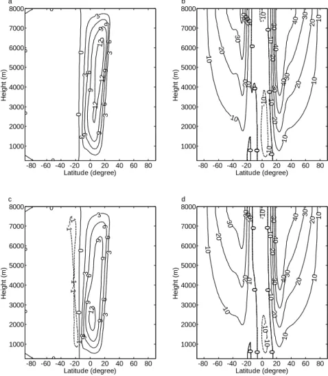
Figure 10.Boreal winter circulation, non-dimensional stream function(a, c)and zonal wind speed (m s−1)(b, d)for the time-dependent simulation withn=2,k=0.5 (upper panels) andn=2,k=3 (lower panels). Dashed lines indicate negative values. Dimensional values of the stream function are obtained by multiplying byνVR ε−1=484 m2s−1.
austral (summer) circulation almost absent. The vertical ex-tent is larger and the maximum is located at higher levels. The summer and winter jets are both more intense than their counterparts fork=3. The tropical easterly winds are in this case stronger than those fork=3 (13.8 m s−1vs. 11.4 m s−1) and the easterly region is also wider. Whenk=3, it is noted that the winter cell is located closer to the Equator than the summer cell.
3.3 A discussion on the casen=2k=1
Whenn=2 andk=1, corresponding to the classic case dis-cussed in many studies, we found that the time-dependent solution is only slightly stronger than the steady solution. Lindzen and Hou (1988) proposed a study of the Hadley cir-culation in which the maximum heating was 6◦off the Equa-tor. In their non-time-dependent model, the solution showed an average circulation much stronger with respect to the equinoctial solution. Lindzen and Hou (1988) suggested that this exceptional strength was due to a nonlinear
amplifica-tion of the annually averaged response to seasonally varying heating, although Dima and Wallace (2003), in a study on the seasonality of the Hadley circulation, did not observe any nonlinear amplification.
With the parameters used for equinoctial and time-dependent simulations, we performed an experiment like that of Lindzen and Hou (1988), with φ0=6◦, which will be
referred to as the solstitial experiment. We found that the winter circulation is stronger by a factor of 3 with respect to the steady solution obtained with the equinoctial heating, consistent with the result of Walker and Schneider (2005). However, the average circulation obtained by averaging two solstitial experiments, with φ0=6◦ and φ0= −6◦,
respec-tively, is only 1.5 times stronger than the steady solution withφ0=0◦, and it has a maximum at the upper levels of
Figure 11.Non-dimensional stream function (contours) and zonal wind speed (m s−1; colors) whenn=2 andk=1 for the steady so-lution (a), annually averaged for the time-dependent solution(b) and averaged for maximum heating 6◦off the Equator(c). Dimen-sional values of the stream function are obtained by multiplying by νVR ε−1=484 m2s−1.
and Schneider (2005), even though a sponge layer actually lowers the maximum stream function height, and we can see the effects of a strong vertical gradient in the upper levels, especially in the time-dependent solution (cf. Figs. 3 and 7). Single solstitial experiments did not show a maximum in up-per levels, as well as the equinoctial and time-dependent ex-periments (Fig. 11a and b). Consequently, the only operation performed to produce Fig. 11c, which exhibits the upper-level maxima, was to average the two solstitial experiments, which causes the maximum at upper levels.
Finally, we notice that comparing the time-dependent so-lution withϕ0=6◦with the equivalent steady solution
hav-ing the heathav-ing off the Equator is not properly correct, since, for the time-dependent model,ϕ0 represents only the
max-imum extension of heating; hence, a more correct compari-son between steady and time-dependent solutions should be performed, with the time-dependent solution havingϕ0=3◦.
In such a case, the average solution is only slightly weaker than the Hadley circulation driven by annually averaged heat-ing or by time-dependent heatheat-ing, which does not show any maximum in the upper levels. Thus, the results of equinoc-tial, time-dependent and solstitial (ϕ0=3◦) experiments are
mutually consistent.
4 Conclusions
The forcing of an Earth-like planet can change for several reasons. For instance, a change in forcing distribution can be caused by different factors such as global warming or long-term variation of solar activity.
Under the assumption of an equal Equator–pole difference at the surface, we used an axisymmetric model to study the sensitivity of the tropical atmosphere to differentθE
distri-butions modulated by two parameters, n that controls the broadness of the distribution andkthat modulates how the θE is distributed vertically. Equinoctial and time-dependent
solutions were simulated and compared. Moreover, for the casen=2 andk=1, corresponding to the classical distribu-tion used in the literature, a few solstitial experiments were also run. Whenn=2 andk=1, the annually averaged cir-culations of equinoctial, time-dependent and solstitial exper-iments are quite close to one another, consistent with the re-sults of Walker and Schneider (2005). However, the rere-sults differ from those of Lindzen and Hou (1988) and Fang and Tung (1999). As in all those works, the maximum of the stream function of the solstitial experiment is at upper levels, but it seems to be related to a spurious effect of the averaging operation rather than a spurious effect due to the rigid lid.
The results provide evidence that concentrated equilib-rium temperature distributions enhance the meridional cir-culation and jet wind speed intensities, confirming findings of Lindzen and Hou (1988), even though these authors im-posed the same energy input. However, in the present study, the concentrated distribution at the Equator has lower energy input.
Vertical stratification is important in determining the posi-tion and intensity of the Hadley cell and jet whennis low, whereas k loses its importance when the θE distribution is
wider. This latter result is consistent with the results of Tan-don et al. (2013), who found that the Hadley cell expansion and jet shift had relatively little sensitivity to the change in the lapse rate. Consequently, the subtropical jet stream inten-sities are controlled by the broadness of horizontal equilib-rium temperature rather than by the stratification, with higher values of the jet when the thermal forcing is concentrated on the Equator. In the case of a time-dependent solution with n=0.5 (concentrated heating) andktaking the extreme val-ues (0.5 and 3), the simulated maximum stream function has the same magnitude order as the observed stream function, 10 times larger than that obtained in HH80 and with the ref-erence simulation, even though with stronger winds too.
The jet stream position does not show any dependence withnandk, except when theθEdistribution is the widest
(n=3); in such a case, an abrupt change occurs and the maximum of the zonal wind jet is located at mid-latitudes (47◦in steady solution and 44◦in an annually averaged time-dependent solution). This behavior can be explained by using the analytic study of this model performed by Cessi (1998), claiming that, when the meridional gradient becomes too small, the circulation behaves as that of a slow rotating planet that exhibits a poleward shift of the subtropical jets.
Acknowledgements. The author thanks two anonymous reviewers
for their insightful comments on the paper, which helped to improve the manuscript, and the editorial staff of Nonlinear Pro-cesses in Geophysics for their valuable work. Helpful discussions with Antonio Speranza, Valerio Lucarini and Renato Vitolo are gratefully acknowledged. The School of Science and Technology, the School of Advanced Studies of the University of Camerino and Fabio Marchesoni are kindly acknowledged for partially funding this publication.
Edited by: V. Perez-Munuzuri Reviewed by: two anonymous referees
References
Allen, R. J., Sherwood, S. C., Norris, J. R., and Zender, C. S.: Re-cent Northern Hemisphere tropical expansion primarily driven by black carbon and tropospheric ozone, Nature, 485, 350–354, 2012.
Caballero, R., Pierrehumbert, R. T., and Mitchell, J. L.: Axisym-metric nearly inviscid circulations in non-condensing radiative-convective atmospheres, Q. J. Roy. Meteorol. Soc., 134, 1269– 1285, 2008.
Cessi, P.: angular momentum and temperature homogenization in the symmetric circulation of the atmosphere, J. Atmos. Sci., 55, 1997–2015, 1998.
Chen, G., Lu, J., and Sun, L.: Delineating the eddy–zonal flow inter-action in the atmospheric circulation response to climate forcing:
Uniform SST warming in an idealized aquaplanet Model, J. At-mos. Sci., 70, 2214–2233, doi:10.1175/JAS-D-12-0248.1, 2013. Dima, I. M. and Wallace, J. M.: On the seasonality of the Hadley
cell, J. Atmos. Sci., 60, 1522–1527, 2003.
Fang, M. and Tung, K. K.: Time-dependent nonlinear Hadley circu-lation, J. Atmos. Sci., 56, 1797–1807, 1999.
Farrell, B. F.: Equable Climate Dynamics, J. Atmos. Sci., 47, 2986– 2995, doi:10.1175/1520-0469(1990)047<2986:ECD>2.0.CO;2, 1990.
Frierson, D. M. W., Lu, J., and Chen, G.: Width of the Hadley cell in simple and comprehensive general circulation models, Geophys. Res. Lett., L18804, doi:10.1029/2007GL031115, 2007. Fu, Q. and Lin, P.: Poleward shift of subtropical jets inferred from
satellite-observed lower stratospheric temperatures, J. Climate, 24, 5597–5603, doi:10.1175/JCLI-D-11-00027.1, 2011. Fu, Q., Johanson, C. M., Wallace, J. M., and Reichler, T.:
En-hanced mid-latitude tropospheric warming in satellite measure-ments, Science, 312, 1179, doi:101126/science.1125566, 2006. Gastineau, G., Le Treut, H., and Li, L.: Hadley circulation
changes under global warming conditions indicated by cou-pled climate models, Tellus, 60, 863–884, doi:10.1111/j.1600-0870.2008.00344.x, 2008.
Gitelman, A. I., Risbey, J. S., Kass, R. E., and Rosen, R. D.: Trends in the surface meridional temperature gradient, Geophys. Res. Lett., 24, 1243–1246, 1997.
Greenwood, D. R. and Wing, S. L.: Eocene continental climates and latitudinal temperature gradients, Geology, 23, 1044–1048, 1995.
Held, I. M. and Hou, A. Y.: Nonlinear axially symmetric circula-tion in a nearly inviscid atmosphere, J. Atmos. Sci., 37, 515–533, 1980.
Hou, A. Y. and Lindzen, R. S.: The influence of concentrated heat-ing on the Hadley circulation, J. Atmos. Sci., 49, 1233–1241, 1992.
Hu, Y. and Fu, Q.: Observed poleward expansion of the Hadley circulation since 1979, Atmos. Chem. Phys., 7, 5229–5236, doi:10.5194/acp-7-5229-2007, 2007.
Johanson, C. M. and Fu, Q.: Hadley cell widening: Model simula-tions versus observasimula-tions, J. Climate, 22, 2713–2725, 2009. Kang, S. M. and Polvani, L. M.: The interannual
rela-tionship between the latitude of the eddy-driven jet and the edge of the Hadley Cell, J. Climate, 24, 563–568, doi:10.1175/2010JCLI4077.1, 2011.
Kim, H.-K. and Lee, S.: Hadley cell dynamics in a primitive equa-tion model, Part II: Nonaxisymmetric flow, J. Atmos. Sci., 58, 2859–2871, 2001.
Lindzen, R. S. and Hou, A. Y.: Hadley circulations for zonally aver-aged heating centered off the Equator, J. Atmos. Sci., 45, 2416– 2427, 1988.
Liu, J., Song, M., Hu, Y., and Ren, X.: Changes in the strength and width of the Hadley Circulation since 1871, Clim. Past, 8, 1169– 1175, doi:10.5194/cp-8-1169-2012, 2012.
Lu, J., Vecchi, G. A., and Reichler, T.: Expansion of the Hadley cell under global warming, Geophys. Res. Lett., 34, L06805, doi:10.1029/2006GL028443, 2007.
Lu, J., Deser, C., and Reichler, T.: Cause of the widening of the tropical belt since 1958, Geophys. Res. Lett., 36, L03803, doi:10.1029/2008GL036076, 2009.
Nguyen, H., Evans, A., Lucas, C., Smith, I., and Timbal, B.: The Hadley circulation in reanalyses: Climatology, variability, and change, J. Climate, 26, 3357–3376, 2013.
Polvani, L. M., Waugh, D. W., Correa, G. J. P., and Son, S.-W.: Stratospheric ozone depletion: the main driver of 20th century atmospheric circulation changes in the Southern Hemisphere, J. Climate, 24, 795–812, doi:10.1175/2010JCLI3772.1, 2011. Santer, B. D., Thorne, P. W., Haimberger, L., Taylor, K. E., Wigley,
T. M. L., Lanzante, J. R., Solomon, S., Free, M., Gleckler, P. J., Jones, P. D., Karl, T. R., Klein, S. A., Mears, C., Nychka, D., Schmidt, G. A., Sherwood, S. C., and Wentz, F. J.: Consistency of modelled and observed temperature trends in the tropical tro-posphere, Int. J. Climatol., 28, 1703–1722, 2008.
Schaller, N., Cermak, J., Wild, M., and Knutti, R.: The sensitivity of the modeled energy budget and hydrological cycle to CO2and
solar forcing, Earth Syst. Dynam., 4, 253–266, doi:10.5194/esd-4-253-2013, 2013.
Schneider, E. K.: Axially symmetric steady-state models of the ba-sic state for instability and climate studies. Part II. Nonlinear cal-culations, J. Atmos. Sci., 34, 280–296, 1977.
Schneider, E. K. and Lindzen, R. S.: Axially symmetric steady state models of the basic state of instability and climate studies, Part I: Linearized calculations, J. Atmos. Sci., 34, 253–279, 1977. Seidel, D. J., Fu, Q., Randel, W. J., and Reichler, T. J.: Widening
of the tropical belt in a changing climate, Nat. Geosci., 1, 21–24, 2008.
Sherwood, S. C., Meyer, C. L., Allen, R. J., and Titchner, H. A.: Ro-bust tropospheric warming revealed by iteratively homogenized radiosonde data, J. Climate, 21, 5336–5352, 2008.
Staten, P. W., Rutz, J., Reichler, T., and Lu, J.: Breaking down the tropospheric circulation response by forcing, Clim. Dynam., 39, 2361–2375, doi:10.1007/s00382-011-1267-y, 2011.
Strong, C. and Davis, R. E.: Winter jet stream trends over the North-ern Hemisphere, Q. J. Roy. Meteorol. Soc., 133, 2109–2115, 2007.
Tandon, N. F., Gerber, E. P., Sobel, A. H., and Polvani, L. M.: Understanding Hadley cell expansion versus contraction: In-sights from simplified models and implications for recent ob-servations, J. Climate, 26, 4304–4321, doi:10.1175/JCLI-D-12-00598.1, 2013.
Titchner, H. A., Thorne, P. W., McCarthy, M. P., Tett, S. F. B., Haim-berger L., and Parker, D. E.: Critically reassessing tropospheric temperature trends from radiosondes using realistic validation experiments, J. Climate, 22, 465–485, 2008.
Waliser, D. E., Shi, Z., Lanzante, J. R., and Oort, A. H.: The Hadley circulation: Assessing NCEP/NCAR reanalysis and sparse in situ estimates, Clim. Dynam., 15, 719–735, 1999.
Walker, C. C. and Schneider, T.: Response of idealized Hadley cir-culations to seasonally varying heating, Geophys. Res. Lett., 32, L06813, doi:10.1029/2004GL022304, 2005.