Optimistic and Pessimistic Forecasts
Vahid Biglari1*, Ervina Binti Alfan1, Rubi Binti Ahmad1, Najmeh Hajian2
1Department of Accounting, Faculty of Business and Accountancy, University of Malaya, Kuala Lumpur, Malaysia,2Department of Accounting, School of Management and Economics, Tarbiat Modares University, Tehran, Iran
Abstract
Previous researches show thatbuy(growth) companies conduct income increasing earnings management in order to meet forecasts and generate positive forecast Errors (FEs). This behavior however, is not inherent insell(non-growth) companies. Using the aforementioned background, this research hypothesizes that since sell companies are pressured to avoid income increasing earnings management, they are capable, and in fact more inclined, to pursue income decreasing Forecast Management (FM) with the purpose of generating positive FEs. Using a sample of 6553 firm-years of companies that are listed in the NYSE between the years 2005–2010, the study determines that sell companies conduct income decreasing FM to generate positive FEs. However, the frequency of positive FEs of sell companies does not exceed that of buy companies. Using the efficiency perspective, the study suggests that even though buy and sell companies have immense motivation in avoiding negative FEs, they exploit different but efficient strategies, respectively, in order to meet forecasts. Furthermore, the findings illuminated the complexities behind informative and opportunistic forecasts that falls under the efficiency versus opportunistic theories in literature.
Citation:Biglari V, Alfan EB, Ahmad RB, Hajian N (2013) The Ability of Analysts’ Recommendations to Predict Optimistic and Pessimistic Forecasts. PLoS ONE 8(10): e73853. doi:10.1371/journal.pone.0073853
Editor:Rodrigo Huerta-Quintanilla, Cinvestav-Merida, Mexico
ReceivedApril 18, 2013;AcceptedJuly 23, 2013;PublishedOctober 1 , 2013
Copyright:ß2013 Biglari et al. This is an open-access article distributed under the terms of the Creative Commons Attribution License, which permits unrestricted use, distribution, and reproduction in any medium, provided the original author and source are credited.
Funding:The authors gratefully acknowledge University research Grant (UM.TNC2/IPPP/UPGP/638/PPP), University of Malaya, Malaysia for support to conduct this research work. The funders had no role in study design, data collection and analysis, decision to publish, or preparation of the manuscript.
Competing Interests:The authors have declared that no competing interests exist. * E-mail: [email protected]
Introduction
Dutta and Gigler [2] suggest that companies have strong incentives to avoid negative Forecast Errors (FEs) or/and generate positive FEs. They propose a contractual model where the management utility is mainly based on whether the reported earnings meet or miss the forecasts. Their theoretical model assumes that both earnings forecasts and earnings management generate positive FEs. It explains and integrates both pessimistic (opportunistic) and optimistic (efficiency) forecasts behavior of companies by illuminating the effect of earnings forecasts on the earnings management.
Abarbanell and Leahvy [1] indicated that the companies’ ability to manipulate earning influences the extent of earnings manage-ment. They argue that the companies with higher growth rates are more capable in manipulating profits. Abarbanell and Leahvy [1] assume that the companies that are recommended by analysts to be bought (hereafterbuycompanies) are classified as growth type companies that will enjoy high profitability. They show that these companies conduct income increasing earnings management in order to meet forecasts and generate positive FEs.
However Abarbanell and Leahvy [1] discovered that the companies recommended by analysts to be sold (hereafter sell companies) are unable to conduct earnings management. Among the reasons for this are that firstly, the sell companies’ stock prices are less susceptible to earnings news, which may render their earnings management ineffective with regards to influencing investors’ decisions. In other words, sell companies cannot effectively manipulate and increase their low profit to boost their
stock prices. Secondly, sell companies possess insufficient sums of available accounting reserves and pre-managed earnings for them to achieve any relevant earning target.
According to Dutta and Gigler [2], sell companies might also suffer from communication restrictions. This seems most logical, as the lack of resources will render sell companies unable to communicate the full scope of their rich information set to investors via the manipulation of reported earnings. Therefore, communication restrictions are binding upon sell companies.
It seems that since sell companies eschew income increasing earnings management, they are both capable and more inclined to pursue income decreasing Forecast Management (FM) to generate positive forecasts errors. Thus, the aim of this research is to examine the effects of the analysts’ recommendations representing the buy and sell companies on the managers’ decisions towards FM.
This research enriches the literature by examining whether sell (non-growth) companies engage in negative FM to realize positive FEs. The importance of the research is that it shows whether analysts’ recommendations in terms of buying or selling of the stocks have informational value that can be used by individual investors to assess the optimism or pessimism of management forecasts. Additionally, the findings obtained here would be useful for future theoretical developments.
discussion and links the findings to the literature. Finally, section 7 concludes the article with a few issues on the implications of policy.
Literature Review
According to Hirst et al. [3], optimism and pessimism of the forecasts are characteristics over which managers are most in control. However, they appear to be the least well-understood components of earnings forecasts, both in terms of theory and empirical research. There are different point of views in the literature on optimism and pessimism of the forecasts. The two dominant views on optimism and pessimism of the forecasts are explained in the following paragraphs.
The first view fits the Watts and Zimmerman [4] opportunistic perspective, and is consistent with criticisms on aligning the management’s interest with an increase in stock prices, which is advocated by Jensen and Meckling [5]. The theories of FM associated with this view have primarily modeled the forecasts as an opportunity that the management will use to pre-empt litigation concerns, influence their reputation, and produce positive FEs while simultaneously influencing stock prices.
Das et al. [6] stated that since stock prices is susceptible to management’s forecasts, the management tend to report a higher forecast. On the other hand, stock prices are highly susceptible to the management’s FE [7,8]. Thus, the more negative the FE is, the more it is perceived as a sign of bad news, and such bad news will most definitely lead to a dramatic fall of stock prices [9,10]. In order to prevent such incidents, the management is inclined to engage in practices called income decreasing FM (or reporting pessimistic forecast) in order to beat forecasts and create positive earnings surprises [11–13].
The second view corresponds to the efficiency perspective. Deegan and Unerman [14] stated that a great deal of positive accounting researches adopted the efficiency perspective. This perspective proposes that managers will choose to use a particular accounting method, as it will most efficiently provide a record of how the organization actually performs. The management will also use forecasts to pass insider information to outsiders. In fact, by forecasting earnings, information asymmetry is reduced, leading to a reduction in the firm’s cost of capital [15].
When the company’s financial position is satisfactory, and the company possesses growth capability (buy companies), the management’s inclination to convey positive (true) information to shareholders will increase, which will increase the manage-ment’s predictions’ optimism [5,16].
Consistent with Dutta and Gigler’s [2] model, for buy companies, the forecasts convey the management’s true expecta-tion to the market, which is followed by income increasing earnings management. However, for the sell companies, the forecasts do not convey true (or optimistic) information to the market, but it is used to dampen the market expectations so that the management can benefit from a positive stock price shock, which is the result of positive earnings surprise.
This research tries to highlight the factor relating to the companies’ growth status that influences the management’s decision to report pessimistic forecast to produce positive FEs when companies’ shares are recommended to sell, and generate optimistic forecast when the companies’ shares are recommended to buy. More specifically, this research tries to determine the ability of analysts’ recommendations (in terms of buy or sell recommendations) in explaining the reason behind FM.
Hypothesis Development
This study aims to examine the effects of the analysts’ recommendations as buy or sell recommendations, representing the growth and non-growth companies on the managers’ decisions towards forecasts management. In order to achieve this aim, four hypotheses have been developed. This section briefly explains the theoretical framework that leads to the hypotheses.
Analysts’ recommendations and pessimistic forecasts (H1)
Dutta and Gigler [2] propose an optimal communication contract where managers who reports high forecasts of income are penalized when such a report is followed by low incomes. The managers who report low forecasts however, are shielded from the risk associated with the reported earnings. They claim that some managers issue high forecasts and subsequently manipulate earnings to realize those forecasts.
Abarbanell and Leahvy [1] conducted an empirical investiga-tion. Depending on whether analysts issue strong sell, sell, buy, and strong buy recommendations, the companies’ stocks are either classified as sell or buy, wherebuycompanies are assumed to be more profitable thansellcompanies.
Buy companies. Abarbanell and Leahvy [1] examined the buy companies and found that firstly, the stock prices of buy companies are susceptible to earnings’ news. Secondly, buy companies can effectively conduct income increasing earnings management. Thus, they show that buy companies issue high forecasts and in order to avoid market punishment, they conduct income increasing earnings management to realize those forecasts. This income increasing earnings management in buy companies is consistent with Dutta and Gigler [2] proposition, which shows earnings’ management being observed only following a high forecast.
Sell companies. However, sell companies pursue a different strategy. Sell companies are considered low profit companies, rendering them unable to effectively conduct income increasing earnings management [1]. This assumption is due to the following reasons; firstly, since sell companies are less vigilantly monitored by investors, their stock price are less susceptible to earnings news [17], making their earnings management ineffective in influencing investors’ opinions [1]. In other words, sell companies cannot effectively manipulate and increase low profit to increase stock prices. Secondly, sell companies are companies that have a meager sum of available accounting reserves and pre-managed earnings to realize any relevant earnings target [1].
Taking into account the aforementioned issues, it seems that unlike buy companies, if sell companies issue high forecasts, they cannot conduct effective earnings management to realize the forecasts afterward, and it is more than likely that they miss the forecasts. Therefore, to prevent this from happening, sell companies prefer to issue low forecasts. Therefore, the first hypothesis would be:
H1: Sell companies issue more pessimistic forecasts than Buy companies.
Analysts’ Recommendations and Frequency of Positive Forecast Errors (H2)
management (company) status, the management engage in FM to avoid negative FEs [13,18].
Buy companies are growth companies and enjoy high profits. Missing the forecasts in the buy companies will inevitably lead to a decrease in the stock’s price. However, sell companies usually suffer from poor earnings performance, which would be a glaring evidence of managerial incompetence [1]. Missing the forecasts for sell companies would cost managers the support of stockholders, and potentially, their very own jobs [19,20].
Since failure in realizing forecasts exposes the sell companies to severe risks, namely, litigation risk, contract termination risk and takeover risk [19,21,22], sell companies are expected to meet their forecasts and avoid the negative FEs more than their counterparts. Thus, it is expected that sell companies have higher frequency of positive FEs than buy companies, therefore, the second hypothesis would be:
H2: Sell companies have higher frequency of positive forecast errors than buy companies.
Forecast Management and Meeting the Forecasts (H3 and H4)
Brown and Caylor [11] stated that investors unambiguously reward firms for reporting earnings that meet their forecasts and penalize firms for reporting earnings that misses their forecasts.
The companies that analysts recommend to sell (sell companies) are the companies that does not have high growth capabilities and suffer from poor performance, which would be a glaring evidence of managerial incompetence [1]. These companies are already affected by the unsatisfactory conditions of the stock market, and if they miss forecasts, they risk further deterioration of the market state. However, unlike the buy companies, the sell companies do not possess enough resources, and have less accounting flexibility to manipulate the profit and meet their respective forecasts. Hence, sell companies seek an alternative method to meet the forecasts.
Therefore, if the company is in the sell position, the management may issue lower forecasts in order to dampen the expectation of outsiders [23]. Based on the result of the firm’s ordinary operations, the management would then report an earning that is equal to or higher than the forecast (report positive forecast error), as doing so will raise the bids for the company’s stocks, and subsequently, increase the company’s stock price.
This provides enough incentives for sell companies to decrease their forecasts in order to create future positive FEs.
Thus, if FM in sell firms is effectively conducted to realize positive FE, then companies that meet forecasts should have conducted higher income decreasing FMs than the companies that miss forecasts. Following this assumption, the following hypotheses for sell companies should be supported.
H3: In sell companies, companies that meet forecasts have done more income decreasing FM than companies that do not meet forecasts.
For buy companies, it is important to meet the forecasts, as negative forecast errors cause negative shocks in the stock price. Buy companies have high profitability, and therefore have enough resources to manipulate earnings [1,2], and can efficiently manage earnings to meet their forecasts.
Thus, in the buy companies, companies that meet forecasts do not necessarily conduct income decreasing FM to meet forecasts.
Thus, we expect the fourth hypothesis for the buy companies to be supported.
H4: There is not significant difference in income decreasing FM between buy companies that meet forecasts and those that do not meet forecasts.
Materials and Methods
Models
The Relationship of Analysts’ Recommendations and Forecast Management (H1). The first hypothesis will be tested by running the regression of FM on the Analysts’ Recommendations (AR), including moderator variables (Learning effect and Difficulty) and several control variables, and the reason for the usage and measurement process of will be explained in section 4.4.
Prob(Down~1)~F(a0za1ARza2AR|Difficultyz
a3AR|FREQza4LMVza5MBza6Hightechz
a7Lag Lossze)
ð1Þ
Where,
Down =1 if company does income decreasing FM (FM is negative) andDown = 0otherwise
AR= the Analysts’ recommendations that takes the value of 1 to 5 (Section 4.2.1)
Difficulty= Difficulty to assess the credibility of management’s forecasts
FREQ= frequency of FM in the previous four years as index of learning effect
LMV= Logarithm of market value MB= Market to Book value
Hightech= 1 if the firm is in one of the high technology industries such as pharmaceuticals, aircraft and spacecraft, medical, preci-sion and optical instruments, radio, televipreci-sion and communication equipment, office, accounting and computing machinery, and 0 otherwise.
Lag_loss= 1 when a firm’s quarterly earnings report preceding the forecast is negative, and 0 otherwise
Taking a page out of Rakow [24], we convertedLMVandMB as indicator variables that are set to one, if the value of the original variable is greater than or equal to the sample median, or zero otherwise.
Using dummy variables instead of continuous variables allows a
1in equation (1) to be interpreted as the effect of the independent
variable when the dummy variable is equal to zero, while a4 througha7can be interpreted as the effect of each variable when the dummy variable is equal to one.
The Relationship of Analysts’ Recommendations and Frequency of Forecast Errors (H2). H2 is tested by running the following logit regression:
Prob(meet~1)~F(a0za1ARza2FREQza3Difficultyz
a4LMVza5MBza6DAza7Hightechza8Lag lossze) ð2Þ Where,
DAis the firm’s ability to manipulate earnings, as reflected by its discretionary accruals, which makes it ideal as a control variable. We use a version of the cross-sectional modified Jones model which is introduced by Ye [25] for the purpose of estimating discretionary accruals.
Other variables are similar to what was explained for equation (1).
The Relationship of forecast management and forecast errors (H3 and H4). For the purpose of testing H3, the ANOVA will be used to test the difference of the mean value of FM between the companies that meet or miss forecasts in sell companies.
We will do the same test for buy companies in order to test the fourth hypothesis.
Variables
There are three types of variables, such as independent, dependent and control variables that are being investigated in this study. Their respective measurements are discussed in this section.
Analysts’ Recommendations (Independent Variable). Following Heidle and Li [26], and Abarbanell and Lehavy [1], it is believed that the perception of the companies’ future growth are duly reflected in the analysts’ recommendations. Since analysts’ recommendations fluctuates at levels less than the bid and ask spread [27] and ask and bid prices [26], it would remain unaffected by market sentiments, and it is assumed that it would be more reliable in capturing the company’s growth perspective.
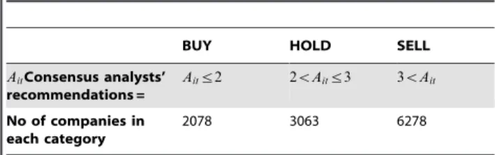
Analysts’ recommendations come in five forms, namely strong buy, buy, hold, sell and strong sell. The rating assigned to each recommendation is displayed in Table 1.
Following Abarbanell and Lehavy [1], this research uses outstanding average (consensus) recommendations at the end of each day in the first, middle and last three weeks of the first month of the fourth quarter. The average recommendation for firmi, on datetis assumed to beAit.
Following Abarbanell and Lehavy [1], each observation is placed in one of the three categories. The first category consists of firms where Ait#2 (denoted ‘‘Buy’’ stocks), the second category
includes firms where 2,Ait#3 (‘‘Hold’’ stocks), while the third
contains the least favorably recommended firms, where Ait.3
(‘‘Sell’’ stocks).
The number of buy and sell companies and the criteria for dividing them are shown in Table 2. In order to compare means (ANOVA tables) in section 5.3, since the extreme growth (buy) and non-growth (sell) companies are taken into account, the hold companies are omitted.
Forecast Management (H1) (Dependent Variable). Foll-owing Burgstahler and Eames [7] and Matsumoto [28], the proxy for FM is measured as follows:
DEPSijtq
Pijtq{4
~b0ijzb1ijt
DEPSijtq{1
Pijtq{5
zb2ijtCRETijtqzeijtq ð3Þ
Where,
Subscripts refer to firmi, industry codej, quarterq, and yeart, and
DEPSijtq= earnings per share changes between the current quarter and four quarters prior.
Pijtq= price per share of common equity, and
CRETijtq= cumulative daily excess returns from three days after
the four quarters prior earnings announcement to 20 days before the current quarter earnings announcement.
b1ijtandb2ijt= the coefficients of the regression.
Similar to Matsumoto [28], (1) the model for each firm-year is estimated using all of the firm quarters of the year from the same industry, except those firms for which the parameters are estimated; (2) only firm-years with 10 or more firm-quarters of data in the same industry are included in the estimation, and (3) observations with variable values in the top and bottom half per cent of the respective distributions are omitted in order to mitigate the impact of extreme values on the parameter estimates. Then, the obtained parameter estimates were used to determine the expected earnings changes from the prior firm year’s fourth quarter:
E(DEPSijtq)~b0ij{1zb1ijt{1(DEPSijtq{1)z
b2ijt{1(CRETijtq)Pijtq{4
ð4Þ
This expected change is added to earnings per share from the same quarter in the prior year in order to obtain the expected forecast of the current quarter’s earnings:
E(Fijtq)~EPSijtq{4zE(DEPSijtq) ð5Þ
Consequently, in order to obtain the expected forecast of annual earnings, we estimated the fourth quarter expected earnings (from equation (5)), and added the prior three quarters of earnings realizations. We took into account the differences between the last reported forecast, and the model-derived expected forecast as a proxy for FM. In order to avoid including preannouncements, forecasts that has been reported near the end of the year have been excluded from the sample.
Table 1.Recommendations and their assigned ratings.
Recommendations Strong
buy buy hold Sell
Strong sell
Rating 1 2 3 4 5
doi:10.1371/journal.pone.0073853.t001
Table 2.The number of company years with buy, hold and sell recommendations.
BUY HOLD SELL
AitConsensus analysts’
recommendations =
Aitƒ2 2vAitƒ3 3vAit
No of companies in each category
2078 3063 6278
The company years are divided to buy, hold and sell categories on the basis of consensus analysts’ recommendations.
FM~Reported Forecast{E(Fijtq) ð6Þ
Forecast Errors (H2) (Dependent Variable). According to Fang [29], Rogers and Stocken [30] and Xu [31], FE is calculated using the following formula:
FE~ (Forecasted EPS{Reported EPS)
Share price of the company at the end of 4th Quarter ð7Þ
Forecasted EPS is the last forecast of the EPS that is reported by the management to the market.
Learning Effect (Moderating - Control Variable). The market may learn from a firm’s FM behavior over a period of time [30]. If the market discerns from a firm’s history that it has habitually engaged in downward FM, they may expect the firms engaging in downward FM in its history to repeat this behavior, and carry out more downward FM than the cleaner firms. Consequently, market expectations will be weakly affected by the current FM. Thus, a rational manager may find it to be in their interest not to frequently manage forecasts downward [30,32].
Therefore, we use a moderating variable, which reflects the frequency of forecast management (FREQ). Depending on the number of times the firm has conducted downward FM in the four previous periods, this variable can have the value of 1, 2, 3, or 4. Difficulty (Moderating -Control Variable). Difficulty re-flects the degree of a market participants’ ability to assess the credibility of the managements’ forecast. According to Rogers and Stocken [30], factor analysis was used on several variables (indicators) for the purpose of identifying the difficulty construct. It is assumed that the indicator specific variances are uncorrelated across variables. Consistent with the goal of predicting FM, all variables are measured prior to the release of the forecasts. The following indicator variables generate a measure of forecasting difficulty [30]:
The standard deviation of analyst forecasts outstanding when the management forecast is released,STD_AF, measures the lack of analysts’ consensus. The standard deviation of the previous analysts’ forecasts errors, scaled by price for five years prior to the forecast release, STD_AFE, proxies for the difficulties analysts experienced when predicting earnings. It is more difficult to forecast a firm’s earnings when the firm is unprofitable compared to when it is profitable. In order to recognize this asymmetry, the indicator Lag-Loss equals to 1 when a firm’s quarterly earnings report preceding the forecast is negative, and 0 if otherwise. Also, the indicator of Predict-Loss equals 1 when the management forecast of earnings is negative, and 0 if vice versa. The standard deviation of the daily stock price for 120 days before the forecast date was measured and denoted as STD_RET. A firm’s bid-ask spread is expected to increase with uncertainty regarding the firm’s forthcoming earnings announcement (see [33]).
Table 3 reports the results of the factor analysis, when the continuous indicators of forecast difficulty are winsorized at 1 and 99 percent levels.
All of the significant correlations among the indicators possess their expected signs. The Difficulty latent variable is estimated by using Principal Axis Factoring (PAF). Standard factor analysis heuristics (e.g., scree-plots and eigenvalues) suggested three factors, and after accounting for the sign and magnitude of the factor loadings, the first factor is extracted as a measure of forecast difficulty.
The values for difficulty ranges from20.58 to 0.84, where the lower value for this variable represent less difficulty for market
participants to assess the credibility of management’s forecasts, while higher values are indicative of higher level of difficulties.
Other Control Variables. One of the other control variable is the threat of litigation. Soffer et al.[34] stated that firms in a litigious environment want to prevent a large disappointment in the earnings announcement date, and this might be better accomplished by providing a less optimistic or even pessimistic forecast shortly before the earnings release date.
Kasznik and Lev [35] posits that firms in high-tech industries face higher risk of litigation as they experience larger price fluctuations, which might translate into potential losses to the investors. Similarly, Baginski et al. [36] used the high-tech industries to control the potential firm-specific litigation risks. The earnings of high-tech firms are more volatile, and inherently carry greater risks of inaccurate forecasts; all these factors could affect a firm’s cost of capital. Therefore, a negative coefficient is predicted vis-a`-vis high-tech, implying that high technology firms issue less optimistic forecasts.
In addition, similar to Rogers and Stocken [28], market to book value (MB), and loss in the previous period (Lag_loss) are used as control variables.
Data and sample
The company’s stock trading information, along with the forecast data, is gathered from the Bloomberg database. The potential market that was considered for data collection is companies in the New York Stock Exchange (NYSE).
The Bloomberg database is used to identify 14414 annual financial statements that were released between January 2005 and December 2010. From this number of companies, the AR for 11419 companies were made available (table 2).
Since firms in regulated industries are more likely to have different incentives than non-regulated industries [28], regulated industries, including utilities, transportation companies, and financial services are excluded from the sample [37,38]. Compa-nies with insufficient data in Bloomberg database are also excluded.
Among the remaining company-years, the Bloomberg database was searched for management earnings estimates, and actual (realized) earnings. The database was also searched for data regarding the analysts’ recommendations, along with other relevant financial data pertaining to this work.
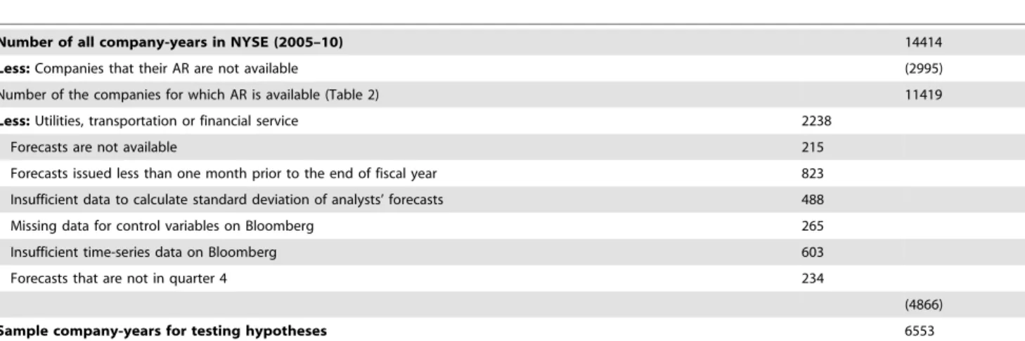
Based on the availability of the aforementioned data, and to carry out prediction tests, which involves examining forecasts reactions to analysts’ recommendations, a subsample of 6553 forecasts were used. The sample selection procedure is summa-rized in Table 4.
The hypotheses were tested in two subsamples. The first subsample was 6553 company-years, while the second subsample was 2449 company-years, which were in the vicinity of zero forecast errors. The reason for using the second subsample is explained in section 5.
Findings
than that for the firms just failing to meet expectations by a small margin, whereas the benefit to firms that beat expectations is only marginally larger than that of the firms that just barely meet expectations. This argument implies that firms that just meet expectations are more likely to have conducted FM, compared to firms that just fail to meet expectations and firms that do beat expectations.
Therefore, the main statistical tests are divided into two parts. In the first part, the hypotheses are tested by taking into account all of the involved company-years (first subsample). In the second part, the hypotheses are tested by considering the company-years that are in the vicinity of zero forecast errors (second subsample).
Since the distance near zero forecast error should be very small, and also since enough number of companies should be considered for analysis, the distance of 0.5 standard deviation of forecast error
on the left and right side of zero forecast error is taken as small distance around zero FE.
Relationship of analysts’ recommendations and forecast management (H1)
Table 5 reports the results for the logistic regression analysis of FM (equation 6).
The interaction termARandFREQis used to measure the effect of learning from historical FM on the relationship betweenARand FM. Thus, the algebraic expression for equation (5) is thata
1is
positive. However, the algebraic expression of learning effect is that a3 is negative and significant. Within this specification, the
coefficient of FM toARshould bea
1+a36FREQ.
The coefficient of FM to AR for a non-difficult firm is a1. However, the coefficient of FM toARfor a difficult firm isa1+a2.
Table 3.Correlation Matrices and Factor Loadings for Forecast Difficulty Measure.
Panel A: Correlation Matrix for Forecast Difficulty Indicators
STD-AF STD-AFE Lag_Loss Predict-Loss STD-Ret Spread
STD-AF 0.001 0.033* 0.052* 0.330** 0.001
STD-AFE 20.001 20.031 20.075 0.970** 0.320**
Lag-loss 20.014 0.144** 0.104** 20.036 0.051*
Predict-loss 0.077** 0.050 0.104** 20.054 20.050
STD-Ret 0.330** 0.954** 0.171** 20.029 0.954**
Spread 0.019 0.740** 0.188** 0.160** 0.748**
Panel B: Factor Loadings
Indicator STD-AF STD-AFE Lagged-loss Predict-loss STD-Ret Spread
Factor Loading 0.065 0.997 0.015 20.021 0.997 0.118
Standardized Factor Score 0.039 0.958 0.112 20.39 0.954 0.854
Panel C: Test of appropriateness of factor analysis
Total Variance Explained 68.30% Bartlett’s Test of Sphericity Chi-Square 50690
Kaiser-Meyer-Olkin Measure of Sampling Adequacy
.620 Sig. 0.000**
*, **Significant at 5% and 1% level.
Table 4.Sampling procedure.
Number of all company-years in NYSE (2005–10) 14414
Less:Companies that their AR are not available (2995)
Number of the companies for which AR is available (Table 2) 11419
Less:Utilities, transportation or financial service 2238
Forecasts are not available 215
Forecasts issued less than one month prior to the end of fiscal year 823
Insufficient data to calculate standard deviation of analysts’ forecasts 488
Missing data for control variables on Bloomberg 265
Insufficient time-series data on Bloomberg 603
Forecasts that are not in quarter 4 234
(4866)
Sample company-years for testing hypotheses 6553
Taking into account Table 5 for the first subsample, the coefficient ofARis positive and significant at a 5% level, for the second subsample, the coefficient ofARare positive and significant at a 1% level. This implies that when theARfor the company is high (i.e. the company is in sell position), the companies conduct higher income decreasing FM compared to when theAR is low (the company is in buy position). The coefficients ofAR6Difficulty are significantly positive in both subsamples (subsample of all company-years and subsample of company-years, which are near zero FE), implying that when it is more difficult for analysts and investors to forecast the company’s profit, and thus recognize the credibility of the management forecasts, the management will do more income decreasing FM. Additionally, the coefficient of frequency (AR6FREQ) is significant and negative in the second subsample. This shows that the frequency of the previous year’s FM moderates the relationship betweenARand FM.
Thus, as a result of the significance of the coefficients ofARin both subsamples, it is concluded thatARaffects FM, and the first hypothesis is supported. In addition, difficulty and frequency moderate the relationship betweenARand FM in companies in a small distance around zero FE. This result shows that managers strategically manipulate their forecasts downward, making it more difficult for the market to assess the truthfulness of their disclosure. With respect to control variables, the coefficients oflag_Lossare significantly positive for the first subsample at 0.05 and for the second subsample at 0.1. This means that the companies that experience lagged loss conduct more downward FM compared to other companies. Also, in the case of companies in a small distance around zero FE, the coefficient of LMV is significant at a 0.1 significance level, and possess its expected values. The coefficients on the remaining control variables are rather insignificant.
The marginal effects are analogous to the slope’s coefficients in an OLS regression [35]. The marginal effect for AR is 1.993 and 2.012 for first and second subsamples, respectively, suggesting that
moving from the first to the third quartile ofAR, the probability of meeting or exceeding expectations increases by approximately 99 and 101 percent, respectively. The values of the marginal effects of AR6Difficulty are 2.577 and 1.282 for the first and second subsamples, respectively. They indicated that the companies that the credibility of their management’s forecasts are most difficult to be assessed by market participants, the probability of its FM is approximately 2.57 and 1.28 times more than the least difficult firms.
The Hosmer and Lemeshow test was used to test the fitness of the models. The test result shown in the lower part of Table 5 is not significant for any of the models, confirming the goodness of fit of the models. Additionally, in order to see the robustness of the results, after dropping each one of the control variables, there were no significant changes in the robustness of the model.
In addition, for determining the presence of multicollinearity, the VIF statistics for independent variables in regression (1) (untabulated) demonstrated no sign of high correlation between independent and control variables.
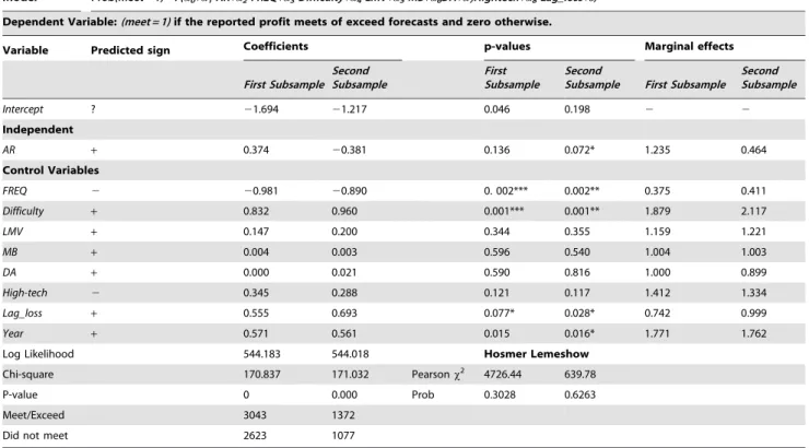
Relationship of analyst’s recommendations and frequency of positive forecast errors (H2)
To examine the relationship of analysts’ recommendations and the frequency of positive FEs, analogous to Matsumoto [26], and by using a cross-sectional logit regression, the regression in equation (2) is estimated (firm and time subscripts have been suppressed):
The results of the logit regressions are indicated in Table 6. In Table 6, the coefficient onARis positive but non-significant for the first subsample, however, for the second subsample, the coefficient of AR is negative and significant suggesting that buy companies are more likely to meet forecasts. Contradicting expectations, in small distance around zero FE, sell companies Table 5.Results for the Management Forecast Bias Hypothesis (Hypothesis 1).
Model Prob(Down = 1) = F(a0+a1AR+a2AR6Difficulty+a3AR6FREQ+a4LMV+a5MB+a6Hightech+a7Lag_Loss+e) Dependent Variable:(Down = 1)if forecast management is negative and(Down = 0)otherwise
Variable Predicted sign Coefficients p-values Marginal effects
First Subsample Second Subsample
First Subsample
Second
Subsample First Subsample Second Subsample
Independents
Constant ? 1.034 21.75 0.276 0.892 2 2
AR + 0.689 0.699 0.01** 0.000*** 1.993 2.012
Control Variables
AR*Difficulty + 3.25 2.662 0. 03*** 0.021** 2.577 1.282
AR*FREQ 2 20.115 20.151 0.114 0.019** 0.891 0.86
LMV + 0.155 0.353 0.422 0.023** 1.167 1.424
M/B 2 20.006 20.003 0.654 0.686 0.994 0.995
Hightech + 20.18 20.181 0.399 0.102 0.835 0.834
Lag_Loss + 0.499 0.739 0.044** 0.098* 1.647 1.538
Log Likelihood 564.693 564.435 Hosmer Lemeshow
Chi-square 57.602 59.383 Pearsonx2 510.36 510.13
P-value 0.000*** 0.000*** Prob 0.243 0.246
Logistic regression results of the first and second subsamples. The coefficients and related t-statistics are estimated by using the following model: Prob(Down = 1) = F(a0+a1AR+a2AR6Difficulty+a3AR6FREQ+a4LMV+a5MB+a6Hightech+a7Lag_Loss+e).
do not possess higher positive forecasts errors. Thus, the second hypothesis is not supported. The reason might be that buy companies might have used income increasing earnings manage-ment strategy to meet the forecasts. In order to produce positive forecasts errors, the income increasing earnings management in buy companies might have been more efficient than income decreasing FMs in sell companies. The coefficient of FREQ is negative and significant at 1% in both subsamples, indicating that if a company has high frequency of income decreasing FM in the previous years, the probability of having positive FE decreases in the current year. This confirms Rogers and Stocken [30] findings that managers have fewer incentives to avoid negative surprises when the frequency of downward FM in previous years is high. Additionally, for both subsamples, the coefficient of Difficulty is positive and significant, which is consistent with Rogers and Stocken [30] notion that managers have more incentives to conduct FM, and thus avoid negative surprises when the recognition of FM is more difficult for investors. The coefficient oflag_lossis negative and significant, consistent with the conjecture that those firms with low value-relevance of earnings have less incentive to avoid negative FEs. The positive but insignificant coefficient of Hightech implies that firms with relatively higher litigation prospects appear to be marginally more likely to avoid negative FEs.
Columns 7 and 8 report the marginal effect of each variable. It is analogous to the slope coefficients in an OLS regression [35]. The marginal effects for frequency are 0.375 and 0.411. These values suggest that moving from the first to the third quartile of FREQdecreases the probability of meeting or exceeding analysts’
expectations by approximately 62.5 and 58.9 percent in the first and second subsamples, respectively. The marginal effect for difficulty equals 1.879 and 2.117 in the first and second subsamples, indicating that an increase in the difficulty of predicting future profits increasing the probability of meeting or exceeding analysts’ expectations by 87 and 111 percent, respec-tively. The marginal effect forLag_lossequals to 0.742 and 0.999, implying that in firms that reported losses in the previous period, the probability of meeting or exceeding analysts’ expectations is lower by 26 and 1 percent in the first and second subsamples, respectively.
Relationship of forecast management and forecast errors in buy and sell companies (H3, H4)
For testing the third hypothesis, the difference of mean values of FM of the companies that possess zero or positive FEs (meet or beat forecasts), and the companies that possess negative FEs (miss forecasts) in sell groups are tested. Columns 3 to 5 of Table 7 show the results of the test.
Tests of differences in mean values of FM between companies that meet or beat forecasts, and the companies that miss forecasts in the group of sell companies showed that there is no significant difference in the mean values of FM between them for the first subsample. However, in the second subsample, the companies that meet forecasts have significantly lower value of FM compared to companies that misses forecasts. This means that in sell companies of subsample 2, the companies that meet or beat forecasts possess more downward FM than companies that fail to meet their forecasts. Thus, in this subsample, H3 is supported.
Table 6.Logit analysis of the probability of meeting or exceeding forecasts and the incentives to avoid negative FEs.
Model Prob(meet = 1) = F(a0+a1AR+a2FREQ+a3Difficulty+a4LMV+a5MB+a6DA+a7Hightech+a8Lag_loss+e) Dependent Variable:(meet = 1)if the reported profit meets of exceed forecasts and zero otherwise.
Variable Predicted sign Coefficients p-values Marginal effects
First Subsample Second Subsample
First Subsample
Second
Subsample First Subsample Second Subsample
Intercept ? 21.694 21.217 0.046 0.198 2 2
Independent
AR + 0.374 20.381 0.136 0.072* 1.235 0.464
Control Variables
FREQ 2 20.981 20.890 0. 002*** 0.002** 0.375 0.411
Difficulty + 0.832 0.960 0.001*** 0.001** 1.879 2.117
LMV + 0.147 0.200 0.344 0.355 1.159 1.221
MB + 0.004 0.003 0.596 0.540 1.004 1.003
DA + 0.000 0.021 0.590 0.816 1.000 0.899
High-tech 2 0.345 0.288 0.121 0.117 1.412 1.334
Lag_loss + 0.555 0.693 0.077* 0.028* 0.742 0.999
Year + 0.571 0.561 0.015 0.016* 1.771 1.762
Log Likelihood 544.183 544.018 Hosmer Lemeshow
Chi-square 170.837 171.032 Pearsonx2 4726.44 639.78
P-value 0 0.000 Prob 0.3028 0.6263
Meet/Exceed 3043 1372
Did not meet 2623 1077
The regression is run on the first and second subsamples. The coefficients and related t-statistics are estimated by using the following model: Prob(meet = 1) = F(a0+a1AR+a2FREQ+a3Difficulty+a4LMV+a5MB+a6DA+a7Hightech+a8Lag_loss+e).
In addition, columns 6 to 8 of Table 7 shows the result of testing the difference in mean values of FM between the companies that possess zero or positive FEs, and the companies that possess negative FEs in the buy group.
Tests of difference in the mean values of FM between companies that meet or beat forecasts, and the companies that miss their forecasts in the group of buy companies showed that there is no significant difference in the mean value of FM between them for the first subsample. For the second subsample, although the difference is significant at a 10% significance level, it is not strong enough to reject the fourth hypothesis. Therefore, H4 is supported.
Discussion
The findings of this research shows that income decreasing FM is more evident in sell firms (H1). Sell companies conduct income decreasing FM to avoid negative forecasts errors and its consequent market punishments that unfavorably affects the management’s utility (H3).
However, avoiding negative forecasts errors via conducting income decreasing FM is not evident in buy firms (H4). This result is consistent with Abarbanell and Lehavy [1], who found that instead of carrying out income decreasing FM, buy companies conduct income increasing earnings management to meet forecasts and produce positive FEs.
Behavior of the buy companies
The findings for (H1) indicate that in buy companies, management conveys less pessimistic forecasts to the market. In addition, the findings for (H4) showed that there is not a significant difference in FM between the buy companies that meet or miss their forecasts. Since for buy companies that have favorable financial records, investors are more responsive to forecasted news, such firms would like to have their private information more fully impounded into their stock prices, and consequently are more capable of reducing information asymmetries in the market, and enjoy lower cost of capital [33,39,40].
Assuming that the management seeks to align market expecta-tions with their own (see Ajinkya and Gift [41]), it is especially true that when the management have extremely promising news to convey [42], and therefore, a favorable track record will be most helpful in enhancing the forecasts’ credibility of buy companies. The reason might be due to the fact that by conveying true information regarding their favorable records, buy companies’
private information, which is usually promising, is fully impounded into their stock prices, and consequently, they are more capable of reducing information asymmetry and enjoy lower costs of capital. Additionally, buy companies are able to do income increasing earnings management to meet the forecasts. Therefore, they need to do less income decreasing FM than sell companies. This might be interpreted as the discovery of the fact that buy companies convey a less pessimistic forecast to the market.
Behavior of the sell companies
The sell companies conduct high income decreasing FM (H1 supported) to realize positive forecasts errors (H3 supported). The reason might be that sell companies issue pessimistic forecasts to avoid the unfavorable utility minimizing consequences of missing forecasts.
In other words, sell companies conduct downward FM to avoid market punishments that results from missing forecasts [16,43]. The reason for this is that as mentioned in section 1 (Introduction), sell companies do not usually generate high economic profits. Therefore, the pessimistic forecasts of sell companies are to avoid market punishments, rather than being opportunistic.
According to Dutta and Gigler [2] framework, the pessimistic forecasts of sell companies might not be due to opportunism. Such pessimism makes their reporting process to be consistent with the efficiency perspective that corresponds with the revelation principle. Therefore, consistent with Dutta and Giggler’s [2] proposition, it is optimal to render income increasing earnings management potentially costly for sell (non-growth) companies, so that they do not report delusive optimistic forecasts.
Conclusion
This research adds to the literature by finding an additional factor that affects management decisions toward issuing forecasts. It has been found that the companies’ growth statuses that are represented by analysts’ recommendations (as buy or sell recommendations) can affect the managements’ decision to conduct FM.
This study helps to understand the mixed findings in the management forecasts literature. While the previous studies suggested that management forecasts are opportunistic, and the management uses the forecasts to manage the analysts’ forecasts [44,45] and affect the stock prices [46], there are several other studies that showed that since management’s forecast conveys insider information to the outsiders, it helps to lessen information Table 7.Test of difference in mean forecast management for the companies that meet management forecasts and the companies that miss forecasts in the Sell (H3) and Buy (H4) companies.
Sell Buy
No. Mean STDEV No. Mean STDEV
Positive or zero FE FM First Subsample 2764 20.0067 0.105 936 20.0012 0.0768
FM Second Subsample 908 27.09E-03 0.0080 394 5.59E-03 0.00658
Negative FE FM First Subsample 2593 0.0032 0.15 828 0.0065 0.1128
FM Second Subsample 732 7.68E-03 0.0135 298 2.46E-02 0.01338
ANOVA’s F Sig. ANOVA’s F Sig.
FM First Subsample 0.098 0.756 1.222 0.274
FM Second Subsample 5.1830 0.023** 2.7457 0.098*
asymmetry, hence decreasing costly litigation of the stockholders against the company [16,43]. It also helps the company to have clear and transparent financial reporting [3,12]. This study adds to the mixed findings in the literature by demonstrating that the management’s forecasts contains a bias that is predictable, taking into account the analysts’ recommendations about the company.
This research is practically useful, as it extends the existing knowledge regarding the information content of the management’s forecasts that affect decisions of the users of the financial information. The findings warn investors to carefully evaluate the management’s forecasts on the basis of whether the companies have buy and sell recommendations before they form their expectations about the company. The findings suggest that the information regarding the analysts’ recommendations might contain important implications for FM, as they might convey informational values that can be used by researchers or even investors.
While the present study reveals some significant points in terms of reliability and accuracy of management forecasts, the findings should neither be overestimated nor underestimated. Gathering data from different markets and from different time periods, and using different FM measurement models might illuminate the issue of the reliability of management forecasts.
Acknowledgments
The authors would like to thank Professor Ali Saeedi from Taylor’s University and, Professor Tan Hun Tong from Nanyang Technological University, and conference participants at the International Conference on Business and Economic Research for their helpful comments.
Author Contributions
Conceived and designed the experiments: VB EBA. Analyzed the data: VB RBA. Wrote the paper: VB EBA NH.
References
1. Abarbanell J, Lehavy R (2003) Can stock recommendations predict earnings management and analysts’ forcast errors. Journal of Accounting Research 41: 1– 31.
2. Dutta S, Gigler F (2002) The effect of earnings forecasts on earnings management. Journal of Accounting Research 40: 631–655.
3. Hirst E, Koonce L, Venkataraman S (2008) Management earnings forecasts: A review and framework. Accounting Horizons 22: 315–338.
4. Watts RL, Zimmerman JL (1978) Towards a positive theory of the determination of accounting standards. The Accounting Review 53: 112–134. 5. Jensen MC, Meckling WH (1976) Theory of the Firm: Managerial Behavior,
Agency Costs and Ownership Structure Journal of Financial Economics3: 305– 360.
6. Das S, Kyonghee K, Sukesh P (2008) An Analysis of Managerial Use and Market Consequences of Earnings Management and Expectation Management AAA 2009 Financial Accounting and Reporting Section (FARS) Paper. Available: http://ssrn.com/abstract = 1270841.
7. Bartov E, Givoly D, Hayn C (2002) The rewards to meeting or beating earnings expectations. Journal of Accounting and Economics 33: 173–204.
8. Kasznik R, McNichols MF (2002) Does meeting earnings expectations matter? Evidence from analyst forecast revisions and share prices. Journal of Accounting Research 40: 727–759.
9. Burgstahler D, Dichev I (1997) Earnings management to avoid earnings decreases and losses. Journal of Accounting and Economics 24: 99–126. 10. Degeorge F, Patel J, Zeckhauser R (1999) Earnings Management to Exceed
Thresholds. Journal of Business Finance & Accounting, 72 1–33.
11. Brown LD, Caylor ML (2005) A Temporal Analysis of Quarterly Earnings Thresholds: Propensities and Valuation Consequences. The Accounting Review 80: 423–440.
12. Gong G, Li LY, Xie H (2009) The Association between Management Earnings Forecast Errors and Accruals. The Accounting Review 84: 497–530. 13. Kasznik R (1999) On the association between voluntary disclosure and earnings
management. Journal of Accounting Research 57: 57–81.
14. Deegan C, Unerman J, editors (2006) Financial Accounting Theory. London: The McGrow-Hill Companies.
15. Lev B, Penman SH (1990) Voluntary forecast disclosure, nondisclosure, and stock prices. Journal of Accounting Research: 49–76.
16. Hui KW, Matsunaga S, Morse D (2009) The impact of conservatism on management earnings forecasts. Journal of Accounting and Economics 47: 192– 207.
17. Barua A, Legoria J, Moffitt JS (2006) Accruals Management to Achieve Earnings Benchmarks: A Comparison of Pre-managed Profit and Loss Firms. Journal of Business Finance & Accounting 33: 653–670.
18. Xin B (2007) Earnings Forecast, Earnings Management, and Asymmetric Price Response: University of Toronto - Joseph L. Rotman School of Management. 19. Beniluz Y (2007) Management earnings forecasts and simultaneous release of
earnings news. Unpublished Working Paper Rutgers, The State University of New Jersey.
20. DeAngelo LE (1988) Managerial competition, information costs and corporate governance: the use of accounting perforemance measures in proxy contests. Journal of Accounting and Economics 10: 3–36.
21. Kim JW, Shi Y (2011) Voluntary disclosure and the cost of equity capital: Evidence from management earnings forecasts. Journal of Accounting and Public Policy 30: 348–366.
22. Frost C (1997) Disclosure policy choices of U.K. firms receiving modified audit reports. Journal of Accounting and Economics 23: 163–187.
23. Li E, Wasley C, Zimmerman J (2010) A Unified Framework of Management Earnings Forecasts: Voluntary, Opportunistic and Disclose or Abstain Incentives. Working Paper. University of Rochester.
24. Rakow KC (2010) The effect of management earnings forecast characteristics on cost of equity capital. Advances in Accounting, incorporating Advances in International Accounting 26 37–46.
25. Ye J (2006) Accounting accruals and tests of earnings management. Working Paper: Baruch College.
26. Darke P, Shanks G, Broadbent M (1998) Successfully completing case study research: combining rigour, relevance and pragmatism. Information systems journal 8: 273–289.
27. Frankel R, McNichols M, Wilson GP (1995) Discretionary disclosure and external financing. Accounting Review 70: 135–150.
28. Matsumoto DA (2002) Management’s Incentives to Avoid Negative Earnings Surprises Accounting Review 77: 483–514.
29. Fang VW (2009) The Role of Management Forecast Precision in Predicting Management Forecast Error. Working Paper Rutgers University.
30. Rogers JL, Stocken PC (2005) Credibility of Management Forecasts. Accounting Review 80 1233–1260.
31. Xu W (2010) Do management earnings forecasts incorporate information in accruals? Journal of Accounting and Economics 49: 227–246.
32. Downing C, Sharpe S (2003) Getting Bad News Out Early: Does it Really Help Stock Prices? working paper. Washington: Federal Reserve.
33. Coller M, Yohn TL (1997) Management Forecasts and Information Asymmetry: An Examination of Bid-Ask Spreads. Journal of Accounting Research 35: 181– 191.
34. Soffer LC, Thiagarajan SR, Walther BR (2000) Earningsp reannouncement strategies. Review of Accounting Studies 5: 5–26.
35. Kasznik R, Lev B (1995) To warn or not to warn: Management disclosures in the face of an earnings surprise. Accounting review: 113–134.
36. Baginski SP, Hassell JM, Kimbrough MD (2002) The effect of legal environment on voluntary disclosure: Evidence from management earnings forecasts issued in US and Canadian markets. The Accounting Review 77: 25–50.
37. Desai H, Rajgopal S, Venkatachalam M (2004) Value-Glamour and Accruals Mispricing: One Anomaly or Two? The Accounting Review 355–385. 38. Riley M (2007) Accounting Information and Analyst Forecast Errors: A study of
teh Explanatory Power of Discretionary Accruals and Accruals Quality. Texas: Texa Tech University.
39. King R, Pownall G, Waymire G (1990) Expectations adjustment via timely management forecasts: Review, synthesis, and suggestions for future research. Journal of accounting Literature 9: 113–144.
40. Verrecchia RE (2001) Essays on disclosure. Journal of Accounting and Economics 32: 97–180.
41. Ajinkya BB, Gift MJ (1984) Corporate managers’ earnings forecasts and symmetrical adjustments of market expectations. Journal of Accounting Research 22: 425–444.
42. Beyer A, Cohen DA, Lys TZ, Walther BR (2010) The financial reporting environment: Review of the recent literature. Journal of Accounting and Economics 50: 296–343.
43. Lennox CS, Park CW (2006) The informativeness of earnings and manage-ment’s issuance of earnings forecasts. Journal of Accounting and Economics 42: 439–458.
44. Cotter J, Tuna I, Wysocki PD (2006) Expectations management and beatable targets: How do analysts react to public earnings guidance?. Contemporary Accounting Research 23: 593–624.
45. Libby R, Hunton JE, Tan HUNT, Seybert N (2008) Relationship incentives and the optimistic/pessimistic pattern in analysts’ forecasts. Journal of Accounting Research 46: 173–198.