A framework to utilize turbulent flux measurements for mesoscale models and remote sensing applications

(1)

HESSD

8, 5165–5225, 2011

An upscaling framework

W. Babel et al.

Title Page

Abstract Introduction

Conclusions References

Tables Figures

◭ ◮

Back Close

Full Screen / Esc

Printer-friendly Version Interactive Discussion

Discussion

P

a

per

|

Dis

cussion

P

a

per

|

Discussion

P

a

per

|

Discussio

n

P

a

per

|

Hydrol. Earth Syst. Sci. Discuss., 8, 5165–5225, 2011 www.hydrol-earth-syst-sci-discuss.net/8/5165/2011/ doi:10.5194/hessd-8-5165-2011

Hydrology and Earth System Sciences Discussions

This discussion paper is/has been under review for the journal Hydrology and Earth System Sciences (HESS). Please refer to the corresponding final paper in HESS if available.

A framework to utilize turbulent flux

measurements for mesoscale models and

remote sensing applications

W. Babel1, S. Huneke2, and T. Foken1

1

Department of Micrometeorology, University of Bayreuth, 95440 Bayreuth, Germany

2

Anemos GmbH, Bunsenstraße 8, 21365 Adendorf, Germany

Received: 16 May 2011 – Accepted: 18 May 2011 – Published: 25 May 2011

Correspondence to: W. Babel (wolfgang.babel@uni-bayreuth.de)

(2)

HESSD

8, 5165–5225, 2011

W. Babel et al.

Title Page

Tables Figures

◭ ◮

Back Close

Full Screen / Esc

Discussion

P

a

per

|

Dis

cussion

P

a

per

|

Discussion

P

a

per

|

Discussio

n

P

a

per

|

Abstract

Meteorologically measured fluxes of energy and matter between the surface and the atmosphere originate from a source area of certain extent, located in the upwind sec-tor of the device. The spatial representativeness of such measurements is strongly influenced by the heterogeneity of the landscape. The footprint concept is capable of

5

linking observed data with spatial heterogeneity. This study aims at upscaling eddy co-variance derived fluxes to a grid size of 1 km edge length, which is typical for mesoscale models or low resolution remote sensing data.

Here an upscaling strategy is presented, utilizing footprint modelling and SVAT mod-elling as well as observations from a target land-use area. The general idea of this

10

scheme is to model fluxes from adjacent land-use types and combine them with the measured flux data to yield a grid representative flux according to the land-use dis-tribution within the grid cell. The performance of the upscaling routine is evaluated with real datasets, which are considered to be land-use specific fluxes in a grid cell. The measurements above rye and maize fields stem from the LITFASS experiment

15

2003 in Lindenberg, Germany and the respective modelled timeseries were derived by the SVAT model SEWAB. Contributions from each land-use type to the observations are estimated using a forward lagrangian stochastic model. A representation error is defined as the error in flux estimates made when accepting the measurements un-changed as grid representative flux and ignoring flux contributions from other land-use

20

types within the respective grid cell.

Results show that this representation error can be reduced up to 56 % when ap-plying the spatial integration. This shows the potential for further application of this strategy, although the absolute differences between flux observations from rye and maize were so small, that the spatial integration would be rejected in a real situation.

25

Corresponding thresholds for this decision have been estimated as a minimum mean absolute deviation in modelled timeseries of the different land-use types with 35 W m−2 for the sensible heat flux and 50 W m−2for the latent heat flux. Finally, a quality flagging

(3)

HESSD

8, 5165–5225, 2011

W. Babel et al.

Title Page

Tables Figures

◭ ◮

Back Close

Full Screen / Esc

Discussion

P

a

per

|

Dis

cussion

P

a

per

|

Discussion

P

a

per

|

Discussio

n

P

a

per

|

scheme to classify the data with respect to representativeness for a given grid cell is proposed, based on an overall flux error estimate. This enables the data user to in-fer the uncertainty of mesoscale models and remote sensing products with respect to ground observations. Major uncertainty sources remaining are the lack of an adequate method for energy balance closure correction as well as model structure and parameter

5

estimation, when applying the model for surfaces without flux measurements.

1 Introduction

Long-term modelling of ecosystem fluxes between the terrestrial surface with its par-ticular vegetation and the atmosphere are now widely used facilities of the scientific communities. The need for that arises not only from the desire for better understanding

10

of ecosystem processes, but also from society’s request for water and greenhouse gas budgets. Within these data networks the eddy covariance (EC) method stands out as the method of choice, utilized within large flux networks with the mentioned objectives like FLUXNET (Baldocchi et al., 2001). A typical feature of such projects is the spa-tial integration of flux data in order to derive budgets for entire ecosystem types (e.g.

15

Jung et al., 2009). While observations are too scarce for regional estimates, integration can be achieved via remote sensing data and mesoscale modelling using flux data as the ground truth. These applications work on grid sizes of at least 1 km edge length. Therefore the point measurements have to be related to a certain grid cell, reflecting its properties. The representativeness of the data depends on the heterogeneity within

20

this area, but also on the heterogeneity within the footprint of the measurements. As upscaling is a problem occurring almost everywhere in earth science, there are lots of approaches to the issue of proper aggregation. The nonlinearity between pro-cesses and driving variables, as well as spatial heterogeneity, pose a major chal-lenge for these approaches (Chen et al., 2009). While simple parameter aggregation

25

(4)

HESSD

8, 5165–5225, 2011

W. Babel et al.

Title Page

Tables Figures

◭ ◮

Back Close

Full Screen / Esc

Discussion

P

a

per

|

Dis

cussion

P

a

per

|

Discussion

P

a

per

|

Discussio

n

P

a

per

|

methods available (e.g. Hasager and Jensen, 1999). Promising approaches stem from coupling of models, given that coupling occurs via fluxes (Best et al., 2004), and mo-saic or subgrid approaches (Avissar and Pielke, 1989; M ¨olders et al., 1996) should be favoured over parameter averaging wherever possible. A sound basis for estimation of representativeness error, related to both measurement footprints and grid size, is

5

the sensor location bias given by Schmid (1997); Schmid and Lloyd (1999). Further methods were proposed by Tolk et al. (2008), who calculate a representation error of a course grid cell as the standard deviation of carbon dioxide fluxes from the respective finer grid cells. They aim at scales beginning from grid cells with an edge length of 2 km up to 100 km. Only a few recent papers combine the scale of EC measurements

10

and remote sensing data or mesoscale models in a physical way, i.e. by utilization of footprint or SVAT modelling. Some studies develop parameterization schemes for re-gional fluxes from observations aided by high resolution remote sensing data (e.g. Su, 2002; Ma et al., 2006). Recently, Chen et al. (2009) have offered a scaling method-ology based on the footprint climatmethod-ology of EC field sites and high resolution remote

15

sensing data. They found better agreement between remotely sensed and EC derived gross primary production (GPP) by weighting the former with the footprint climatology than by equal weighting of the grid cells. This approach was also applied to a Chinese field site (Chen et al., 2010).

The footprint approach, which has recently been widely accepted, relates

mea-20

sured data to its sources. It is expected to play a crucial role for matching the scales of EC measurements and remote sensing data or mesoscale models (e.g. Schmid, 1997). Schmid (2002) and Vesala et al. (2008) offer sound overviews of the existing concepts. Validation concepts exist as well (Foken and Leclerc, 2004), but this is-sue has yet to be investigated (Vesala et al., 2008). Comparisons in G ¨ockede et al.

25

(2005) and Kljun et al. (2002) show better performance of Lagrangian stochastic mod-els over analytical modmod-els. Further comparisons of Lagrangian stochastic modmod-els with LES (Large Eddy Simulation) model predictions on a basis of 2-D footprint func-tions showed good agreement for intermediate measurement heights and convective

(5)

HESSD

8, 5165–5225, 2011

W. Babel et al.

Title Page

Tables Figures

◭ ◮

Back Close

Full Screen / Esc

Discussion

P

a

per

|

Dis

cussion

P

a

per

|

Discussion

P

a

per

|

Discussio

n

P

a

per

|

conditions (Markkanen et al., 2009). Also Finn et al. (1996) and Hsieh and Katul (2009) assign reasonable performance to the Lagrangian stochastic forward model approach on step change heterogeneity, even if this model type is only valid for horizontal homo-geneous flow conditions due to the inverted plume assumption. However, not all flow characteristics can be tackled by the footprint concept, as Foken and Leclerc (2004)

5

state that influences of remote obstacles on measurements have been found, even if the disturbed region is beyond the predicted source area. But nevertheless, footprint analysis was combined with measurement quality in order to characterise complex study sites (G ¨ockede et al., 2004, 2006). This scheme was applied successfully for CarboEurope sites (Rebmann et al., 2005; G ¨ockede et al., 2008) and on the Tibetan

10

Plateau (Metzger et al., 2006). Similar procedures were also conducted for FLUXNET sites by Chen et al. (2009), but the scope was more quantitative and hints at the upscal-ing issue: monthly and annual uncertainties in EC fluxes from a 59-year-old Douglas-fir stand were attributed to variations in footprint climatology and estimated to be approx-imately 15–20 %. The authors state that footprint-weighted EC fluxes can be used to

15

estimate the bias between spatially-explicit ecological models and tower-based remote sensing at finer scales.

The aim of this study is to combine footprint analysis and SVAT modelling to enhance representativeness of EC-measured turbulent fluxes on a grid level of 1 km edge length, which is a typical size for mesoscale models assisted by moderate resolution remote

20

sensing data. Such models are utilized for comprehensive assessment of energy and water budgets on a regional scale. This approach is useful for field sites with high sen-sor location biases, where differences in fluxes from various patches are expected to exceed model uncertainties. The need for such algorithms is underpinned by e.g. Avis-sar (1995); Raupach and Finnigan (1995); Baldocchi et al. (2005); Kim et al. (2006). In

25

(6)

HESSD

8, 5165–5225, 2011

W. Babel et al.

Title Page

Tables Figures

◭ ◮

Back Close

Full Screen / Esc

Discussion

P

a

per

|

Dis

cussion

P

a

per

|

Discussion

P

a

per

|

Discussio

n

P

a

per

|

for this case study and its results are presented including considerations about uncer-tainty. Finally the implications are summarized in Sect. 5.

2 Methods

2.1 Site description

The investigated datasets were gathered within the LITFASS-2003 experiment from

5

19 May to 17 June 2003, in a rural landscape around the Meteorological Observatory Lindenberg of the German Meteorological Service (DWD) and its boundary-layer field site Falkenberg, 52◦10′01′′N and 14◦07′27′′E (Beyrich and Adam, 2007). Fourteen micrometeorological stations were operated over different surfaces, mainly agricultural crops and forests, aiming at evapotranspiration estimates over heterogeneous

land-10

scapes (Beyrich and Mengelkamp, 2006; Mengelkamp et al., 2006). Weather condi-tions were fairly dry during LITFASS-2003, interrupted only by scarce rainfall episodes, which led to a huge variability of water availability and evapotranspiration (Beyrich and Mengelkamp, 2006).

For this investigation, datasets were used from three adjacent farmland sites (from

15

North to South: A4, A5 and A6). While there was no obstacle between A4 and A5, A5 and A6 were separated by a track with a hedgerow. Serving as cropland, A5 was cultivated with rye, and A4 and A6 with maize, during the LITFASS-2003 campaign. All sites were equipped as a full energy balance station, the turbulent fluxes were mea-sured using a Campbell CSAT3 sonic anemometer and a Campbell KH20 hygrometer

20

for A4, a Metek USA-1 sonic anemometer together with a KH20 for A5 and a CSAT3 in combination with a LI-COR LI-7500 CO₂/H₂O gas analyser for A6. Further measure-ments include radiation with all components for A5 (Kipp & Zonen CNR1 net radiome-ter) and A6 (Eppley PIR Pyrgeometer, Kipp & Zonen CM24 albedomeradiome-ter), while for A4 only downwelling short-wave radiation (Campbell SP1110) and net radiation (REBS

25

Q7) were recorded. Soil heat flux as well as soil temperature and moisture profiles

(7)

HESSD

8, 5165–5225, 2011

W. Babel et al.

Title Page

Tables Figures

◭ ◮

Back Close

Full Screen / Esc

Discussion

P

a

per

|

Dis

cussion

P

a

per

|

Discussion

P

a

per

|

Discussio

n

P

a

per

|

were obtained by various instruments (Rimco CN3, Hukseflux HFP, REBS HFT, Camp-bell 107 Probe, Pt100 and IMKO Trime EZ). Additional site-specific plant physiological and physical parameters such as leaf area index (LAI), canopy height and soil texture were recorded during the campaign, for details see Mauder et al. (2006).

As the campaign was conducted during a growing phase of the respective cereals,

5

canopy height and therefore displacement height and roughness length varied through-out the experiment. For A5 (rye), canopy height began with 90 cm, peaking with 150 cm on 2 June with a final height of 130 cm, recorded on 12 June. A6 (maize) exhibits a much larger variability, starting with 9 cm which could roughly be attributed to bare soil conditions, and growing continuously to 60 cm on 10 June as the last record. Nearly

10

the same pattern shows A4 (maize) with canopy heights ranging from 5 cm to 75 cm.

2.2 Postprocessing of turbulent flux data

The dataset of half-hour turbulent fluxes (n=1392) was calculated using the software package TK2 (Mauder and Foken, 2004), and the processing of LITFASS-2003 data is described in detail in Mauder et al. (2006). Turbulent fluxes were filtered, excluding

15

fluxes with poor quality (data with quality flags of 7–9 were excluded using a scheme ranging from 1 to 9 by Foken et al., 2004). Fetch analysis by Mauder et al. (2006) revealed homgeneous flow conditions and no internal boundary layers for A5 and neg-ligible influence on A4 within the measurement heights z_m=2.9 m and z_m=3.25 m, respectively. The A6 (maize) turbulence complex, however, was situated near the track

20

accompanied by a hedgerow, leading to a disturbed flow field for a wind sector from WNW to ENE. Consequently, A6 data was filtered for the disturbed sector. Further-more, the contribution of the target land-use was determined by footprint analysis (see Sect. 2.3), the respective half-hour flux values were excluded depending on wind direc-tion and stratificadirec-tion and using a threshold of 80 % for the target contribudirec-tion, which

25

poses a representative measurement after G ¨ockede et al. (2008).

(8)

HESSD

8, 5165–5225, 2011

W. Babel et al.

Title Page

Tables Figures

◭ ◮

Back Close

Full Screen / Esc

Discussion

P

a

per

|

Dis

cussion

P

a

per

|

Discussion

P

a

per

|

Discussio

n

P

a

per

|

of the three sites used here ranged from 60 % to 70 % of the available energy, while the SVAT (Soil – Vegetation – Atmosphere – Transport) scheme used in this study closes the energy balance by definition (see Sect. 2.4). This fact compromises direct compar-isons of turbulent flux observations and modelled fluxes, as already shown for these sites by Kracher et al. (2009). Therefore the sensible and the latent heat flux are

cor-5

rected following Twine et al. (2000) as suggested in Foken (2008): the residualRes of the energy balance is distributed among the turbulent fluxes while the Bowen ratioBo

was preserved yielding the energy balance corrected heat fluxesQH,EBCandQE,EBC. In

order to avoid unreasonable huge corrections and artificial spikes, the correction was not applied whenBowas negative or at least one of the turbulent fluxes fail to exceed

10

the measurement accuracy, which was assumed to be 10 W m−2 in absolute values. Instead, such values were excluded from further analysis.

After all filtering and energy balance correction, missing values sum up to 58–63 % forQH,EBCandQE,EBC, and an even higher missing fraction in the case of A6 due to the

wind sector filtering. Most of these gaps, however, occur during the night, where from

15

experience the fluxes are known to be low. Although this fact is somewhat comforting, it raises the need for gapfilling to obtain unbiased results of mean fluxes on a daily ba-sis or longer time scales. Therefore the energy balance corrected turbulent fluxes are gapfilled with calibrated SVAT model runs for further analysis. The calibration proce-dure is described in Sect. 2.4 and the influence of gapfilling on the results is discussed

20

in Sect. 4.4.

2.3 Footprint analysis

In this study a Lagrangian stochastic forward model is used to estimate two-dimensional contributions of source areas. While a general description of the model is given by Rannik et al. (2003), it is used with a simplified parameterisation of turbulent

25

flow according to conditions for low vegetation as used in G ¨ockede et al. (2005). As La-grangian stochastic models require high computational costs, source weight functions

(9)

HESSD

8, 5165–5225, 2011

W. Babel et al.

Title Page

Tables Figures

◭ ◮

Back Close

Full Screen / Esc

Discussion

P

a

per

|

Dis

cussion

P

a

per

|

Discussion

P

a

per

|

Discussio

n

P

a

per

|

for each half-hour measurement were picked from precalculated tables following a pro-cedure as used in G ¨ockede et al. (2004, 2008).

As a forward model depends on the inverted plume assumption, horizontal homo-geneity is required in principle. Experiences from past investigations and validations, however, affirm its applicability even under heterogeneous conditions (e.g. Rebmann

5

et al., 2005; G ¨ockede et al., 2005, 2008; Markkanen et al., 2009, 2010). Further limits stem from flow distortion due to large obstacles like hedges, creating flow patterns and internal boundary layers which cannot be resolved by this model.

2.4 SVAT modelling

As the proposed upscaling scheme needs additional modelling, a SVAT scheme called

10

SEWAB, developed by Mengelkamp et al. (1999) in the former GKSS Research Center, Geesthacht, Germany, is implemented. This model has been chosen due to its energy balance closure technique, which was well rated in a comparison study of Kracher et al. (2009). Here only the principles of the model structure will be highlighted in the following, for further information see the publications mentioned above as well as

15

Kracher et al. (2009). The application and derivation of model parameters is described in Sect. 2.4.2.

2.4.1 SEWAB model structure

Momentum flux (u_∗) and sensible heat flux (QH) were calculated using a bulk approach

u_∗= q

CD·u(z) (u(0)=0) (1)

20

QH=ρ·cp·CH·u(z)·(Tg−T(z)) (2)

with the drag coefficientCD, the Stanton numberCHandcpas the specific heat

(10)

HESSD

8, 5165–5225, 2011

W. Babel et al.

Title Page

Tables Figures

◭ ◮

Back Close

Full Screen / Esc

Discussion

P

a

per

|

Dis

cussion

P

a

per

|

Discussion

P

a

per

|

Discussio

n

P

a

per

|

on aerodynamic and thermal roughness lengths as well as atmospheric stratification following Louis (1979). For the latent heat flux QE a bulk approach also applies in

analogy to Eq. (2) in general, but the flux is split up into evaporation from bare soil and vegetated surface flux, the latter again composed of evaporation from wet foliage and transpiration from dry foliage. While for evaporation from bare soil and wet foliage

5

the Dalton number equals the Stanton number CH, the transpiration drag coefficient

was parameterised with the aerodynamic resistance and the stomatal resistance after Noilhan and Planton (1989). Similar, the soil heat fluxQG is estimated by

QG=λ

T_g−TS1

∆z_S1

!

(3)

with the thermal conductivityλand the first soil layer temperatureTS1with a thickness 10

of ∆zS1=2 cm. Soil temperature distribution is described by the diffusion equation

and vertical soil water movement is governed by the Richards equation. Relationships between soil moisture characteristics were used from Clapp and Hornberger (1978). The net radiation is written as

Q∗_R=−Rswd(1−a)−Rlwd+εσTg4 (4)

15

with the albedoa, the emissivityε, the Stefan-Boltzmann constantσand the net radi-ation Q∗_R. Downwelling short-wave and long-wave radiation (Rswd and Rlwd) were not

parameterised for this dataset but prescribed as a part of the forcing data. Finally, the energy balance is given by

−Q∗_R=QH+QE+QG (5)

20

which is closed in SEWAB by definition. While all components are given with separate equations without using the balance equation, the closure is achieved by an iteration of the surface temperatureTguntil the residual disappears. Thus, instead of charging one

flux to serve as balance residual, the discrepancy is shared by all fluxes sensitive to T_g. Directly affected areQH,QG, and the upwelling long-wave radiation (see Eqs. (2), 25

(3) and (4)), but alsoQEvia the temperature dependent specific humidity of saturation.

(11)

HESSD

8, 5165–5225, 2011

W. Babel et al.

Title Page

Tables Figures

◭ ◮

Back Close

Full Screen / Esc

Discussion

P

a

per

|

Dis

cussion

P

a

per

|

Discussion

P

a

per

|

Discussio

n

P

a

per

|

2.4.2 SEWAB parameter estimation

The model runs were achieved with two different sets of parameter for each station, an optimised and a “realistic” set. The former are intended to show a maximum fit to the existing data for gapfilling (Sects. 2.2, 3.2). The parameters were optimised simultane-ously for QH,EBC and QE,EBC with the coefficient of efficiency serving as the objective 5

function (see Eq. (10)) using a SCE-UA (Shuffled Complex Evolution University of Ari-zona) algorithm (Duan et al., 1992, 1994) followed by a MOSCEM-UA (Multiobjective Shuffled Complex Evolution Metropolis – University of Arizona) algorithm (Vrugt et al., 2003). This procedure was applied to SEWAB just as described in detail by Johnsen et al. (2005). The performance of these runs and their influence on the uncertainty of

10

the upscaled fluxes is discussed in Sect. 4.4.

The realistic parameters were estimated using the detailed information gathered by Kracher et al. (2009). The goal of these model runs is to transfer knowledge of the target land-use, where measurements exist, to an unknown adjacent land-use type by adjusting the site specific parameters (see also Sect. 3.2). As a consequence,

param-15

eter optimisation is not appropriate: it is very unlikely to allow estimation of parameters suitable for transferring to other land-use types, even if the physical basis of the model might be correct, due to the problem of equifinality. For this purpose it would be cru-cial to find a best strategy for adapting model structure and parameters, but this task goes beyond the scope of this work. Only to show in-principle feasibility of this goal,

20

the parameters were taken nearly unchanged from the realistic sets in Kracher et al. (2009) as an “unbiased” estimate, because they did not compare the results with en-ergy balance corrected measurements. An overview of the most important parameter gives Table 1. As A4, like A6, contained maize and showed the same growth pat-tern during the LITFASS-2003 campaign, both parameter sets differ only slightly in

25

(12)

HESSD

8, 5165–5225, 2011

W. Babel et al.

Title Page

Tables Figures

◭ ◮

Back Close

Full Screen / Esc

Discussion

P

a

per

|

Dis

cussion

P

a

per

|

Discussion

P

a

per

|

Discussio

n

P

a

per

|

according to the ARNO concept, or depth dependent saturated hydraulic conductivity (Mengelkamp et al., 1999, 2001) are switched off as they all contain parameters for which it is problematic to find realistic values. Furthermore, the roughness lengths are originally assessed from the measurements. In order to exclude this information, z0

is assumed to be one-tenth of the canopy height. Unfortunately the minimum

stom-5

atal resistanceR_s,min, estimated as 300 s m− 1

for wheat (source: Altman and Dittmer, 1966) and applied for A5, lead to far too low Q_E compared to the observed Q_E_,_EBC. While this estimate may be reasonable for an individualTriticum aestivumplant, more recent, modelling oriented, studies tend to lower values, e.g. Schulze et al. (1994) give 90 s m−1 for cereals (sample size: 5) or Alfieri et al. (2008) with 23–25 s m−1 for two

10

winter wheat fields with intermediate precipitation. Thus, estimates for Rs,min differ

quite a lot and moreover, Ingwersen et al. (2011) argue for a variableR_s,min. Therefore

we decided to select a uniformRs,minfor all sites and choose 60 s m

−1

for A5, which is the same value as used for maize. And lastly, the LAI value from Kracher et al. (2009) for the maize field (A4 and A6), 1.5, seemed to be estimated for the total surface.

15

Therefore the value was scaled with the inverse fraction of vegetated area 0.7−1 for a consistent usage in SEWAB. At the end, the parameters for the sites A4 and A6 differ from A5 only in canopy height, roughness length, albedo, LAI, root depth and fraction of vegetated area.

While these parameters are kept constant in the model for the whole measuring

20

period, the real parameters evolved in time as the experiment was conducted during the growing phase and especially the maize sites showed a significant development of canopy height and, consequently, also other parameters in Table 1. This results in a loss of predictive capacity of the model. On the other hand, a broader range of model performance within the dataset is achieved, raising the opportunity of investigating the

25

relationship between model fit and success of the upscaling procedure.

(13)

HESSD

8, 5165–5225, 2011

W. Babel et al.

Title Page

Tables Figures

◭ ◮

Back Close

Full Screen / Esc

Discussion

P

a

per

|

Dis

cussion

P

a

per

|

Discussion

P

a

per

|

Discussio

n

P

a

per

|

2.4.3 SEWAB forcing data

The model is forced with a half-hourly dataset derived by the LITFASS-2003 experiment (see Sect. 2.1) consisting of precipitation, air temperature, wind velocity, air pressure, relative humidity, downwelling short-wave and long-wave radiation. As these standard meteorological variables exist for each of the three sites, the optimised runs were driven

5

by the individual forcing sets in order to obtain the best fit. In contrast, for the evaluation of the upscaling scheme the realistic runs were forced with only one dataset (from A5) as would be the case in prospective application. Nevertheless, the different sets were useful for error estimation as discussed in Sect. 4.4.

2.5 Statistics

10

For evaluation of model performance simple comparisons are carried out using the bias Band the mean absolute error MAE

B=N−1

N X

i=1

(Pi−Oi) (6)

MAE=N−1

N X

i=1

|P_i−O_i| (7)

with O as the observations and P the model predictions. Thus the MAE provides a

15

measure for model performance or model fitting. There is also a need in this study to quantify the differences between two time series of observations and two series of predictions in the same manner as it is done by the MAE, although the last applications measure dissimilarity more than “errors” in the sense of “failure”. In order to avoid confusion with the mean absolute deviation or absolute mean difference, which are

20

(14)

HESSD

8, 5165–5225, 2011

W. Babel et al.

Title Page

Tables Figures

◭ ◮

Back Close

Full Screen / Esc

Discussion

P

a

per

|

Dis

cussion

P

a

per

|

Discussion

P

a

per

|

Discussio

n

P

a

per

|

Dobs :=N−1

N X

i=1

O₁_,i−O₂_,i

(8)

Dmod :=N−1

N X

i=1

P₁_,i−P₂_,i

(9)

withO1,O2as observations andP1,P2as predictions from the respective land-use types

1 and 2. As a goodness of fit measure serves the coefficient of efficiency (CoE) or Nash-Sutcliffe coefficient. Introduced by Nash and Sutcliffe (1970), the CoE reads as

5

follows

NS=1−

N X

i=1

(P_i−O_i)2

N X

i=1

(O_i−O)2

(10)

withOas the mean of the observations. The CoE has a range of [−∞,1] and should not be mistaken for the more common coefficient of determinationR2. Although the general definitions equal each other, R2 is predominantly used to assess model performance

10

between observations and predictors via linear regression by ordinary least squares (Everitt, 2002), and in this case partitioning of the total variance into explained and residual variance does hold, restricting the range ofR2to [0,1].

2.6 Spatial integration of fluxes

The upscaling scheme proposed in this study and described in Sect. 3.2 connects

ex-15

isting QA/QC tools for EC flux measurements with a procedure for spatial integration of fluxes on a grid size of about 1 km edge length, utilizing footprint and SVAT modelling.

(15)

HESSD

8, 5165–5225, 2011

W. Babel et al.

Title Page

Tables Figures

◭ ◮

Back Close

Full Screen / Esc

Discussion

P

a

per

|

Dis

cussion

P

a

per

|

Discussion

P

a

per

|

Discussio

n

P

a

per

|

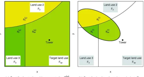
For this task, the relationships between observations, source area and grid represen-tative fluxes should be considered from two perspectives as displayed in Fig. 1. A hy-pothetical grid cell is assumed to containM land-use types, each covering a fractional areaa(_jg) and featuring the specific fluxes F_j,j∈[1,2,...,M]. Typically, measurements are conducted on one use of interest or target use. We define here the

land-5

use type 1 to be the target land-use and the respective fractional areaa(₁g)=a(_targ) and the target land-use fluxF1=Ftar.

The first perspective to consider is the flux for an entire grid cell (Fig. 1a): Letting the land-use specific fluxes Fj and their fractional areas be known, a grid representative

fluxF(g)can be obtained by the tile approach,

10

F(g)= M X

j=1

a(_jg)·F_j (11)

assumingFj to be homogeneous for each land-use type (see Fig. 1a). This approach

has been already applied to the LITFASS-2003 area on a landscape scale (Beyrich et al., 2006).

On the other hand, observations collected on a tower of a given height reflect the

15

properties of a source region in a corresponding upwind distance from the device. This region can be determined by footprint analysis, delivering a source weight function, which essentially assigns a relative contribution to the measured signal for each pixel in the land-use domain according to the resolution of the footprint model. These rela-tive contributions can be aggregated to a fractional weight for each land-use typea(_jf)

20

(Fig. 1b). Then an observed flux Fobs at the tower is related to the land-use specific

fluxes, in analogy to Eq. 11, by

Fobs=

M X

j=1

(16)

HESSD

8, 5165–5225, 2011

W. Babel et al.

Title Page

Tables Figures

◭ ◮

Back Close

Full Screen / Esc

Discussion

P

a

per

|

Dis

cussion

P

a

per

|

Discussion

P

a

per

|

Discussio

n

P

a

per

|

The location and extent of this source area is changing rapidly in time, with its temporal dynamics mainly driven by wind direction and stratification in the surface layer.

3 Upscaling of flux measurements

3.1 Representativeness of flux measurements

In this section we aim to provide a framework for assessing a representation error for

5

flux measurements in a heterogeneous landscape. As stated by Nappo et al. (1982), representativeness is a value judgement and depends on situation and purpose. Con-sequently, we follow Nappo et al. (1982) in general by defining measures for repre-sentativeness error in analogy to the proposed criterion for point-to-area representa-tiveness, but the equations are adapted to the specific problem as follows: We restrict

10

ourselves to a situation we judge to be typical when using EC flux measurements for mesoscale modeling or as ground truth for remote sensing data. Let us consider again the hypothetical grid cell, Fig. 1, as described in Sect. 2.6. Assuming each land-use type to be homogeneous, the real flux from the entire grid can be obtained by Eq. (11). Unfortunately, not all land-use specific fluxesFj required are known in reality, but the

15

measurements provide the flux from areas of target land-use. Although this assumption is often temporally violated, in many casesFtarcan be obtained with a certain accuracy

by cautious quality checks and footprint analysis followed by a gapfilling algorithm. The most simple, but often used, approach for spatial integration is to assume the target land-use to be representative for the whole grid cell:

20

F_tar(g)=Ftar (13)

In contrast, we propose in this study a model-aided grid representative fluxF_mod(g):

F_mod(g) =a(_targ)·Ftar+

M X

j=2

a(_jg)·F_j,mod (14)

(17)

HESSD

8, 5165–5225, 2011

W. Babel et al.

Title Page

Tables Figures

◭ ◮

Back Close

Full Screen / Esc

Discussion

P

a

per

|

Dis

cussion

P

a

per

|

Discussion

P

a

per

|

Discussio

n

P

a

per

|

This flux is composed of Ftar from the measurements and the modelled fluxes

Fj,mod,j∈[2,3,...,M] as a surrogate for the missing Fj. Furthermore, substitution of

F(g) by the surrogatesF_mod(g) orF_tar(g) lead to grid representativeness errors according to Schmid (1997), which can be defined as mean absolute errorsδmod and δtar

respec-tively.

5

δmod=N−1

N X

i=1

F

(g)

i −F

(g) mod,i

(15)

δtar=N−1

N X

i=1

F

(g)

i −F

(g) tar,i

(16)

When evaluating the success of the proposed spatial integrationF_mod(g), one may ask for the advantage of applyingF_mod(g) instead ofF_tar(g), i.e. modelling the fluxes from adjacent land-use types and combining it with the target flux instead of simply usingFtar for the 10

entire grid cell. This can be formulated as an absolute reduction in error (ARE) or in the style of a proportional reduction in error (PRE):

ARE :=δtar−δmod (17)

PRE := δtar−δmod

δtar

(18)

Positive ARE and PRE indicate successful application of the proposed spatial

inte-15

gration (without information regarding significance), negative values indicate thatF_mod(g) performs even worse thanF_tar(g). Unfortunately ARE and PRE can only be calculated, whenF(g)is known, which restricts this evaluation to experimental case studies. Here a case study is constructed with the LITFASS-2003 data set, which is explained in detail in Sect. 4.1.

(18)

HESSD

8, 5165–5225, 2011

W. Babel et al.

Title Page

Tables Figures

◭ ◮

Back Close

Full Screen / Esc

Discussion

P

a

per

|

Dis

cussion

P

a

per

|

Discussion

P

a

per

|

Discussio

n

P

a

per

|

3.2 Upscaling concept

The general idea of the concept is to derive grid representative fluxes by combining the observations from the target area with modelled data from the other land-use types within the grid cell. The workflow of this concept can be divided into three parts: a flux data post processing part, a gapfilling part and a spatial integration part. Furthermore,

5

the second and the third part depend on the site characteristics. We differentiate here between two situations: The measurement tower is located within the land-use of in-terest, or target land-use, in a way that a substantial part of the measurements can be attributed as a pure signal from this land-use type. This will be, furthermore, called the

target case. The opposite is then themixed case, where a pronounced heterogeneity

10

exists around the sensor and most of the data reflects the properties of two or more land-use types. While the target case should be typical for low vegetation landscapes, the mixed case may occur more often for high tower measurements or airborne mea-surements. With respect to the datasets used, we focus in this study on the first, or target, case.

15

3.2.1 Target case: identifiable target land-use

In this section the workflow for the target case is described in detail and displayed in Fig. 2. In the first part state-of-the-art flux corrections and quality assessment as used in Mauder et al. (2006) are conducted. A first footprint analysis delivers the spatial context of flux quality and the fraction of flux contribution from the target area in order to

20

characterize the site (G ¨ockede et al., 2008). Consequently, bad rated data is excluded at this step.

For the second part, the preprocessed flux data has to be filtered according to the land-use contributions to ensure that the flux information stems from one land-use type. A high quality standard for this task may be 80 % or higher contribution from the target

25

area. Now the energy balance closure for the target area can be determined and an energy balance closure correction can be applied, which is implemented after Twine

(19)

HESSD

8, 5165–5225, 2011

W. Babel et al.

Title Page

Tables Figures

◭ ◮

Back Close

Full Screen / Esc

Discussion

P

a

per

|

Dis

cussion

P

a

per

|

Discussion

P

a

per

|

Discussio

n

P

a

per

|

et al. (2000) in this study. After all these steps many data points are discarded, raising the need for gapfilling. Therefore a land surface model is calibrated and validated for the target land-use. Merging this calibrated run with the data yields a full energy balance closed target area fluxFtar.

For spatial integration it has to be checked whether fluxes from other land-use types

5

F_j,j∈[2,3,...,M] within the grid cell of interest are expected to deviate considerably fromFtar. In this case, the land surface model is activated again to simulate the target

land-use with parameter as realistic as possible, yieldingFtar,mod. This model

simula-tion is then transferred to the other land-use typesF_j,mod by appropriate modification of

the site specific parameters. Now spatial integration can be performed with Eq. (14),

10

deliveringF_mod(g) as an estimate for the true grid representative fluxF(g). As true fluxes from adjacent land-use types are unknown, the PRE, Eq. (18), cannot be evaluated. Instead, a surrogate measure can be obtained quantifying the difference between the modelled fluxes Dmod, Eq. (9), and the spatial integration is accepted or rejected

ac-cording to the thresholdX.

15

Dj,mod=N−1

N X

i=1

F_j,_mod_,i−F_tar_,_mod_,i

> X (19)

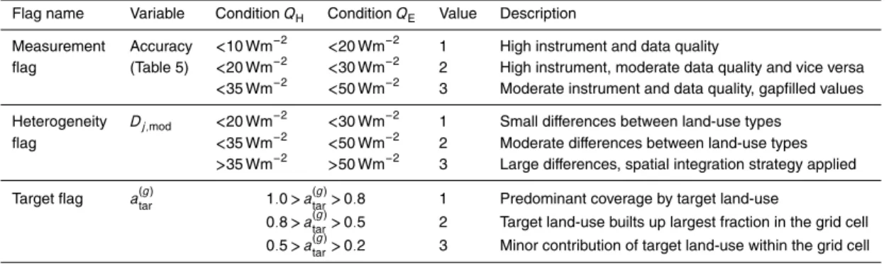
The applicability ofD_j,mod and the threshold value X is discussed in Sect. 4.3. In

any case, quality assessment is conducted with respect to point-to-area and target representativeness (Schmid, 1997; Schmid and Lloyd, 1999). A flagging scheme is proposed in Sect. 4.6

20

3.2.2 Mixed case: pronounced heterogeneity

In this case footprint analysis reveals significant influence of adjacent land-use types on the measured flux andFtar6=Fobs. Again consideringFjto be homogeneous for each

land-use type and the source weight function from the footprint analysis to be real,Fobs

is related to the land-use specific fluxesFj via Eq. (12). The energy balance closure,

(20)

HESSD

8, 5165–5225, 2011

W. Babel et al.

Title Page

Tables Figures

◭ ◮

Back Close

Full Screen / Esc

Discussion

P

a

per

|

Dis

cussion

P

a

per

|

Discussion

P

a

per

|

Discussio

n

P

a

per

|

however, is difficult to assess for a mixed signal and therefore the simulations of tur-bulent fluxes tend to overshootFobs, when applying Eq. (12) to the land-use specific

model runs. Recent studies suggest a connection of this imbalance to surface het-erogeneity and secondary circulations (Foken, 2008; Foken et al., 2010). Therefore a reasonable assumption is that measurements from nearby surface types exhibit a

uni-5

form relative residual of the measurements (i.e. turbulent energy divided by available energy). Under this assumption, the source weight integrated model simulations are proportional toFobs.

Fobs∼

M X

j=1

a(_jf)·Fj,mod (20)

Therefore the right hand side of Eq. (20) can be regressed versusFobs. The resulting 10

modelled fluxes are then the basis for the spatial integration.

4 Results and discussion

4.1 Evaluation concept

In Sect. 3.1 a spatial integration strategy is proposed in Eq. (14) withF_mod(g), composed of the measured flux from the target land-useFtarand modelled fluxes from other land-use 15

types present in the grid cell intended for upscaling. The advantage (or disadvantage) of this approach over simply usingF_tarfor the entire grid cell is given in terms of absolute and proportional reduction in error ARE and PRE, respectively, defined in Eqs. (17)– (18). These measures can only be given if the true fluxes from all land-use types in the grid cell are known. Therefore, a grid cell is considered here with the postprocessed,

20

energy balance closed and gapfilled flux data from LITFASS-2003 sites A4 (maize), A5 (rye) and A6 (maize), see Sects. 2.1, 2.2, as the true fluxesF_j from the respective surfaces. The realistic SEWAB runs (Sect. 2.4.2) were taken to be the modelled fluxes Fj,mod, as they could in principle be derived without flux data.

(21)

HESSD

8, 5165–5225, 2011

W. Babel et al.

Title Page

Tables Figures

◭ ◮

Back Close

Full Screen / Esc

Discussion

P

a

per

|

Dis

cussion

P

a

per

|

Discussion

P

a

per

|

Discussio

n

P

a

per

|

In the case of more than two land-use types within the grid cell (M >2), the PRE and ARE do not only depend on the different fluxes, but also on the respective fractional land-use contributionsa(_jg) (use Eqs. (11), (13)–(16) in Eqs. (17)–(18)). Thus, effects originating from flux differences within the cell may be boosted or weakened according to their contribution. In order to focus on the influence of flux differences, we restrict

5

ourselves to only two land-use types to reveal the relationships more clearly. The annotations forM=2 simplify as follows:

Ftar=F1 Flux from target land-use

Fsur=F2 Flux from surrounding land-use

a(_targ)=a(₁g)

10

a_sur(g) =a₂(g)=1−a(_targ) ARE2=ARE|M=2

PRE2=PRE|M=2

Applying now Eqs. (11), (13)–(16) in Eqs. (17) and (18) forM=2 yields

ARE2=a (g) sur·N−

1

N X

i=1

F_sur_,i−F_tar_,i −

F_sur_,i−F_sur_,_mod_,i =a

(g)

sur·(Dobs−MAEsur) (21) 15

PRE₂=1−

N X

i=1

F_sur_,_mod_,i−F_sur_,i

N X

i=1

F_sur_,i−F_tar_,i

=1−MAEsur Dobs

(22)

In contrast to the general PRE, the PRE₂ is now independent from fractional land-use areas and the ARE2 scales only with 1−a

(g)

tar. Simply speaking, the PRE2 shows

(22)

HESSD

8, 5165–5225, 2011

W. Babel et al.

Title Page

Tables Figures

◭ ◮

Back Close

Full Screen / Esc

Discussion

P

a

per

|

Dis

cussion

P

a

per

|

Discussion

P

a

per

|

Discussio

n

P

a

per

|

error as long as the difference in observationsDobs exceeds the modelling error of the

surrounding land-use MAE_sur, and vice versa. It should be mentioned here, that the PRE2 can be interpreted as a generic and baseline-adjusted coefficient of efficiency,

as proposed by Legates and McCabe (1999). It differs from the originalNSin Eq. (10) by using the sums of absolute errors rather than the sums of squared errors and by

re-5

placingOwithFtaras the so-called baseline series. However, no theoretical distribution

exists for PRE2, which makes it difficult to assess significance, but this problem could

be overcome by bootstrapping techniques (Legates and McCabe, 1999).

In this study no significances were assessed. Instead, intercomparisons between the gapfilled and energy balance corrected measurements of turbulent energy fluxes

10

QH,EBC and QE,EBC from the LITFASS-2003 stations A4 (maize), A5 (rye) and A6

(maize) and respective SVAT model runs were conducted. In the context of the up-scaling scheme proposed in Sect. 3, these fluxes are assumed to be the real fluxes in a grid cell, containing the target land-use (Ftar) and a surrounding land-use (Fsur). The

threshold valuesX proposed in Sect. 3.2.1 were established by evaluating daily PRE₂

15

values in Sect. 4.2 and exploring the relationships toDobsandDmod in 4.3. Finally, the

thresholds were discussed by considering the relevant uncertainties in Sect. 4.4 and the influence of the footprint in Sect. 4.5.

4.2 Model performance

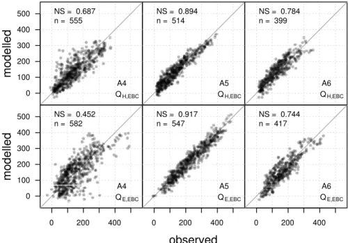
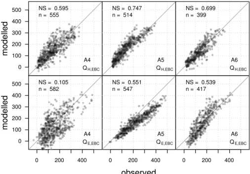
Figure 3 displays the energy balance corrected fluxes vs. the calibrated model runs.

20

The Nash-Sutcliffe coefficient NS (Eq. (10)), shows quite reasonable fits for A4 and A5 with values ranging from 0.74 to 0.92. The performance for A4 is worse, which may be attributed to the special conditions of the site influenced by a forest edge at a distance of 150 m. As “special conditions” are common features in field surveys, this data set improves the study by broadening the range of possible outcomes. Compared

25

to the findings from Kracher et al. (2009), this result indicates that the coherence be-tween observations and model outputs can be significally enhanced by energy balance closure correction, and bias can be reduced. However, the application of the spatial

(23)

HESSD

8, 5165–5225, 2011

W. Babel et al.

Title Page

Tables Figures

◭ ◮

Back Close

Full Screen / Esc

Discussion

P

a

per

|

Dis

cussion

P

a

per

|

Discussion

P

a

per

|

Discussio

n

P

a

per

|

integration requires physically justified parameterisation, and therefore the the fluxes are compared to the realistic model runs as well (Fig. 4). As expected, the realistic runs perform not as well as the calibrated ones, with more bias for all fluxes and poor coherence for A4.

To ensure a consistent averaging for further investigation of daily and summary

5

statistics, all observations are gapfilled with the optimised model runs. While this practice is a necessity for providing average values, some bias might be introduced in the evaluation and evident when comparing model runs with observations, includ-ing gapfilled values derived by another model run. Although large gaps exist due to all postprocessing steps (see Sect. 2.2), most of the gaps occur during nighttime. In

10

relation to the set of turbulent flux data, where the absolute values exceed 10 W m−2, energy balance corrected flux observations constitute up to 78 % for A4, 67 % for A5 and 53 % for A6. The influence of this procedure is discussed in Sect. 4.4.

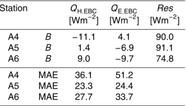
Summary statistics according to the evaluation concept (Sect. 4.1) are given in Ta-ble 2. Shown are mean fluxes for the whole period as well as mean absolute differences

15

between observationsDobs, between simulations of the realistic model runsDmod and

the mean absolute error MAE.

The reduction in error measures ARE2and the PRE2are calculated for each paired

combination of the sites A4 to A6, and the indices (1) or (2) indicate whether the first or the second station of a specific pair is the target land-use. The suboptimal performance

20

of the realistic model run A4, as seen already in the scatterplot (Fig. 4), is reproduced in the MAE with highest values forQH,EBCandQE,EBCat A4 station. Nevertheless, the

PRE₂ for A4 as adjacent land-use and A5 as target land-use shows positive values with 0.43 forQH,EBC and 0.28 forQE,EBC, implying a reduction of representativeness

error by 43 % and 28 %, respectively. The reason for this is, that the fair model fit of A4

25

is compensated by an even larger difference between the observations of A4 and A5. So theDobscan be interpreted as the potential: the more the fluxes between land-use

(24)

HESSD

8, 5165–5225, 2011

W. Babel et al.

Title Page

Tables Figures

◭ ◮

Back Close

Full Screen / Esc

Discussion

P

a

per

|

Dis

cussion

P

a

per

|

Discussion

P

a

per

|

Discussio

n

P

a

per

|

adjacent land-use types. Best PRE2, ranging from 38 % to 56 %, are achieved with A5

and A6 in the grid cell as well as A4 and A5, provided that A4 is the target land-use. For A4 and A6 in a grid box no significant error reduction can be achieved for all fluxes, and in half of the cases it gets even worse. This outcome is expected, as both A4 and A6 contain maize, showed similar dynamics and therefore differ not so much from

5

each other. Comparing the different fluxes,QH,EBC performs best due to better model

fitting thanQE,EBC. The absolute reduction in error ARE2 witha (g)

tar=50 % seem to be

quite low, but one has to keep in mind that in this case study the fluxes do not differ so strongly among the sites, anyhow.

As a surrogate for significance, the PRE2is also evaluated on a daily basis, and the 10

variation of these daily values are displayed in Fig 5. The specific paired combination and the assignment of the target land-use is coded according to a colour scheme. Most of the results for the whole period (Table 2) are confirmed, with distinct positive PRE2

for the turbulent fluxes at combinations (A4, A5) and (A5, A6) and not decisive or even negative values for (A4, A6).

15

4.3 Evaluation of the threshold for spatial integration

The application of the spatial integration includes the modelling of adjacent land-use types, where little or no data is available. TheDmodis suggested in Sect. 3.2.1, Eq. (19)

as a surrogate for the PRE2 in order to accept or reject the spatial integration. Its

applicability and a reasonable thresholdX is discussed in this section, beginning with

20

theD_obsand its relationship to the PRE₂.

The Dobs exhibit a huge temporal variation on a daily basis (not shown), which is

attributed to the temporal evolution of turbulent fluxes due to the rapid growth of the maize fields (A4 and A6). These variations are reflected in daily PRE₂ (see Fig. 5), providing the opportunity to investigate the relationship toDobs, which is displayed in 25

Fig. 6: The scatterplots show dailyDobs versus daily PRE2, the combination of sites

again coded according to a colour scheme and the target land-use specified by the

(25)

HESSD

8, 5165–5225, 2011

W. Babel et al.

Title Page

Tables Figures

◭ ◮

Back Close

Full Screen / Esc

Discussion

P

a

per

|

Dis

cussion

P

a

per

|

Discussion

P

a

per

|

Discussio

n

P

a

per

|

symbols. It is reasonable to assume a coherence between these two variables, be-cause larger differences in observed fluxes raise the potential of successfully replacing an observed flux by a modelled one, a fact which is reflected in PRE2, whereDobs

oc-curs in the denominator (Eq. (22)). In the ideal case, that the daily modelling error for the surrounding land-use MAE_sur(numerator in Eq. (22)) is constant, this coherence is

5

a perfect hyperbolay=1−C/xwith yx−→→∞1 and the modelling error equals theD_obs between observations for PRE₂=0. The displayed ideal lines were drawn using the respective MAEsur (see Table 2) for the whole period as constantC. Now deviations

from the ideal line are explained only by variations in daily MAEsur. It follows that the

outcome of the spatial integration for a whole measurement campaign can be

approx-10

imated withDobs, and the thresholdX is marked by the intersection point of the ideal

line with the x-axis (Fig. 6). Using the maximum intersection points for all combinations from Fig. 6, the thresholds for minimalDobsto obtain a positive PRE2are 24 W m

−2

for QHand 42 W m−

2

forQE.

The PRE2, as used until now, gives an answer to the question of whether modelling 15

errors exceedDobs. For applications of the scheme for the target case, however, only

Ftaris known, and not the fluxes from adjacent areas. Therefore, a surrogate measure

has to be found of whether modelling of the adjacent area was successful. A simple attempt would be to relate the difference in mean modelled fluxes Dmod to PRE2 in

order to see if a similar threshold of minimum differences can be found as for mean

20

observed fluxes. Figure 7 displays the dailyDmod versus PRE2 in the same style and

ideal lines as Fig. 6. It is obvious that theDmod do not reach as high values as the

Dobs, which is also reflected in the values for the whole period (Table 2). The reason

is that the model is not capable of reproducing the whole variance between the fluxes of different sites by changing only a few parameters, as done here (see Table 1). As

25

(26)

HESSD

8, 5165–5225, 2011

W. Babel et al.

Title Page

Tables Figures

◭ ◮

Back Close

Full Screen / Esc

Discussion

P

a

per

|

Dis

cussion

P

a

per

|

Discussion

P

a

per

|

Discussio

n

P

a

per

|

the spatial integration would be rejected, even though the outcome was positive. One has also to keep in mind that the unknown MAEsurof the adjacent land-use has to be

approximated by the model fit of the target land-use MAEtar. In this case study, these

estimates are to some extent unbiased as the parameters were estimated for each site simultaneously without fitting, but they differ quite largely from site to site. But it is

5

reasonable to assume that the model fit will get worse when transferring the parameters to an unknown land-use type. So there should be an independent minimum threshold established, which can be derived by uncertainty estimations.

4.4 Consideration of uncertainties

The application of the proposed upscaling scheme includes many steps, which all may

10

introduce errors in the results. The most significant sources of uncertainty are the uncertainty of the flux data itself and uncertainties due to the energy balance closure correction, the gapfilling and the modelling uncertainty of the spatial integration. As the last two sources depend on modelling, these uncertainties can be discussed in terms of model input uncertainty, parameter uncertainty and uncertainty of the model

struc-15

ture. The uncertainty of the flux data is already widely discussed in the community (e.g. Mauder et al., 2007b). Based on the EBEX-2000 EC sensor comparison experiment, Mauder et al. (2006) give uncertainty estimates from 10 to 30 Wm−2 for QH and 20

to 40 Wm−2 forQE, depending on sonic anemometer types following the

recommen-dations by Foken and Oncley (1995), and on data quality. Hollinger and Richardson

20

(2005) infer the random error of flux measurements by deviations between two nearby instruments and Richardson et al. (2006) from one time series with subsets under sim-ilar conditions. Despite these being substantially different approaches, both yield error quantities similar to Mauder et al. (2006).

(27)

HESSD

8, 5165–5225, 2011

W. Babel et al.

Title Page

Tables Figures

◭ ◮

Back Close

Full Screen / Esc

Discussion

P

a

per

|

Dis

cussion

P

a

per

|

Discussion

P

a

per

|

Discussio

n

P

a

per

|

4.4.1 Uncertainty due to the energy balance closure and gapfilling

The residual of the measured energy balance, given with about 70 % of the available energy for A5 and A6 and only 60 % for A4, constitutes a large potential source of error. In absolute values, the mean residual (without gapfilling) ranges from 75 to 90 Wm−2 during daytime and from−25 to−10 Wm−2during nighttime. Day- and nighttime fluxes

5

were distinguished here by a threshold of 10 Wm−2 forRswd, and the data gaps are

assumed to be independent from flux magnitude for each group in order to give mean values for non-gapfilled time series. The daytime error is expected to be reduced by the correction for energy balance closure according to the Bowen ratio after Twine et al. (2000), which is seen to be the best first guess for this issue (Foken, 2008),

10

although there is no reason to assume scalar similarity between temperature and water vapour transport (Ruppert et al., 2006; Mauder et al., 2007a), and others propose a correction only for QH (Ingwersen et al., 2011). After EBC correction, all missing

values are gapfilled, including those where the EBC correction was not applied due to non-compliance with the requirements (see Sect. 2.2). This leads to a mixed influence

15

of gapfilling and EBC correction for daytime values and no influence of EBC correction on the nighttime values, as nearly no data was corrected due to EBC during night.

In order to disentangle the different error sources, one can set up the following as-sumptions: (i) Although common SVAT models are always a simplification of reality and prone to structural uncertainty, they are in principle able to resemble the true turbulent

20

flux partitioning with a certain accuracy. (ii) The optimisation algorithm used is capable of finding a model solution which approaches this accuracy given the true fluxes. It fol-lows that the gapfilling model would approximate the true fluxes with same accuracy as it approximates the (probably wrong) givenQH,EBCandQE,EBC. Therefore, the daytime

gapfilling error can be expressed as MAE andBbetween the non-gapfilled fluxes and

25

the gapfilling model runs. The turbulent energy fluxes for all stations show maximum MAEs of 36 Wm−2forQHand 51 Wm−

2