Representativeness errors in comparing chemistry transport and chemistry climate models with satellite UV/Vis tropospheric column retrievals

(1)

GMDD

8, 7821–7877, 2015

Comparing models with satellite column

retrievals

K. F. Boersma et al.

Title Page

Abstract Introduction

Conclusions References

Tables Figures

◭ ◮

Back Close

Full Screen / Esc

Printer-friendly Version Interactive Discussion

Discussion

P

a

per

|

Discussion

P

a

per

|

Discussion

P

a

per

|

Discussion

P

a

per

|

Geosci. Model Dev. Discuss., 8, 7821–7877, 2015 www.geosci-model-dev-discuss.net/8/7821/2015/ doi:10.5194/gmdd-8-7821-2015

This discussion paper is/has been under review for the journal Geoscientific Model Development (GMD). Please refer to the corresponding final paper in GMD if available.

Representativeness errors in comparing

chemistry transport and chemistry

climate models with satellite UV/Vis

tropospheric column retrievals

K. F. Boersma1,2, G. C. M. Vinken3, and H. J. Eskes1

1

Royal Netherlands Meteorological Institute, De Bilt, the Netherlands

2

Wageningen University, Meteorology and Air Quality department, Wageningen, the Netherlands

3

Eindhoven University of Technology, Eindhoven, the Netherlands

Received: 26 June 2015 – Accepted: 21 August 2015 – Published: 10 September 2015

Correspondence to: K. F. Boersma (boersma@knmi.nl)

Published by Copernicus Publications on behalf of the European Geosciences Union.

(2)

GMDD

8, 7821–7877, 2015

retrievals

Title Page

Tables Figures

◭ ◮

Back Close

Full Screen / Esc

Discussion

P

a

per

|

Discussion

P

a

per

|

Discussion

P

a

per

|

Discussion

P

a

per

|

Abstract

UV/Vis satellite retrievals of trace gas columns of nitrogen dioxide (NO₂), sulphur diox-ide (SO₂), and formaldehyde (HCHO) are useful to test and improve models of atmo-spheric composition, for data assimilation, air quality hindcasting and forecasting, and to provide top-down constraints on emissions. However, because models and satellite

5

measurements do not represent the exact same geophysical quantities, the process of confronting model fields with satellite measurements is complicated by representative-ness errors, which degrade the quality of the comparison beyond contributions from modelling and measurement errors alone. Here we discuss three types of represen-tativeness errors that arise from the act of carrying out a model-satellite comparison:

10

(1) horizontal representativeness errors due to imperfect collocation of the model grid cell and an ensemble of satellite pixels called superobservation, (2) temporal repre-sentativeness errors originating mostly from differences in cloud cover between the modelled and observed state, and (3) vertical representativeness errors because of reduced satellite sensitivity towards the surface accompanied with necessary retrieval

15

assumptions on the state of the atmosphere. To minimize the impact of these represen-tativeness errors, we recommend that models and satellite measurements be sampled as consistently as possible, and our paper provides a number of recipes to do so. A practical confrontation of tropospheric NO₂columns simulated by the TM5 chemistry transport model (CTM) with Ozone Monitoring Instrument (OMI) tropospheric NO₂

re-20

trievals suggests that horizontal representativeness errors, while unavoidable, are lim-ited to within 5–10 % in most cases and of random nature. These errors should be included along with the individual retrieval errors in the overall superobservation er-ror. Temporal sampling errors from mismatches in cloud cover, and, consequently, in photolysis rates, are on the order of 10 % for NO₂ and HCHO, and systematic, but

25

(3)

GMDD

8, 7821–7877, 2015

retrievals

Title Page

Tables Figures

◭ ◮

Back Close

Full Screen / Esc

Discussion

P

a

per

|

Discussion

P

a

per

|

Discussion

P

a

per

|

Discussion

P

a

per

|

associated with the vertical sensitivity of Ultraviolet-visible (UV/Vis) satellite retrievals. Simple vertical integration of modelled profiles leads to systematically di_fferent model columns compared to application of the appropriate averaging kernel. In comparing OMI NO₂ to GEOS-Chem NO₂ simulations, these systematic differences are as large as 15–20 % in summer, but, again, avoidable.

5

1 Introduction

Chemistry transport models (CTMs) are increasingly being evaluated with satellite col-umn retrievals from UV/Vis solar backscatter satellite instruments. Satellite retrievals of trace gas concentrations constitute a rich source of information on key tropospheric species such as nitrogen dioxide (NO₂), sulphur dioxide (SO₂), and formaldehyde

10

(HCHO) that is beginning to be exploited on an ever-larger scale. Ultraviolet-visible (UV/Vis) satellite observations are being used to:

– evaluate the capability of models to simulate atmospheric concentrations of various species (e.g. Uno et al., 2007; Herron-Thorpe et al., 2010; Huijnen et al., 2010a),

15

– drive data assimilation experiments aimed at improving estimates of the atmo-spheric state (e.g. Wang et al., 2011; Inness et al., 2013; Miyazaki et al., 2014),

– provide constraints on uncertain model inputs such as emission inventories through inverse modelling (e.g, Wang et al., 2007; Müller et al., 2008; Mijling and van der A, 2012; Barkley et al., 2013), to identify new emissions sources (for

in-20

stance newly built power plants, Zhang et al., 2009; and to better understand the formation of secondary pollutants such as ozone, Verstraeten et al., 2015; and aerosol, Veefkind et al., 2011),

– test processes influencing the lifetime of crucial chemical species (e.g. Schaub et al., 2007; Lamsal et al., 2010; Beirle et al., 2011; Stavrakou et al., 2013), or,

25

(4)

GMDD

8, 7821–7877, 2015

retrievals

Title Page

Tables Figures

◭ ◮

Back Close

Full Screen / Esc

Discussion

P

a

per

|

Discussion

P

a

per

|

Discussion

P

a

per

|

Discussion

P

a

per

|

more broadly, the chemical regime of the atmosphere (e.g. Martin et al., 2004; Duncan et al., 2010)

When comparing model simulations to satellite measurements, both modelling errors and measurement errors are usually taken into account. Measurement errors are often reasonably well characterized (e.g. Boersma et al., 2004; De Smedt et al., 2008; Lee

5

et al., 2009), but modelling errors are more difficult to establish, because of the large number of uncertain model processes, uncertain boundary (e.g. emissions) and ini-tial conditions, and unresolved or misrepresented aspects of atmospheric physics and chemistry. Modelling errors are best characterized by comparing model simulations to observations. Unfortunately, the observations available for such comparisons are

10

mostly limited in vertical range and regional coverage such as in the case of ground-based networks, or they are merely sporadic in space and time, such as for aircraft campaigns. Satellite data records are based on robust retrieval methods, provide global coverage, and cover decadal time spans. Satellite data has recently been successfully used for dedicated modelling error studies (e.g. Lin et al., 2012; Stavrakou et al., 2013).

15

When using satellite data, modellers need to be aware that most UV/Vis-retrievals generally contain little information on the vertical distribution of a species (the exception is stratospheric ozone profile retrieval in the far UV of the spectrum, but this species will not be considered in this study). Here we focus on the application of tropospheric UV/Vis retrievals, and we limit ourselves to retrievals of tropospheric species NO₂, SO₂,

20

and HCHO for comparison with models. These species are all relatively short-lived and their retrievals are generally based on differential optical absorption spectroscopy (DOAS, Platt and Stutz (2008)). DOAS retrievals in the UV/Vis match relevant absorp-tion cross secabsorp-tion spectra to the solar backscatter spectrum measured by the satellite instrument in order to infer the column integral (slant column density, expressed in

25

(5)

GMDD

8, 7821–7877, 2015

retrievals

Title Page

Tables Figures

◭ ◮

Back Close

Full Screen / Esc

Discussion

P

a

per

|

Discussion

P

a

per

|

Discussion

P

a

per

|

Discussion

P

a

per

|

of the species, and surface properties. When these assumptions are very different from the atmospheric state modelled by a chemistry transport model (CTM), this will lead to inflated differences between modelled (by, say, CTM 1) and retrieved columns (aided by CTM 2). Such differences, however, can be avoided or in any case minimized, if the user of satellite data accounts for the representativeness and averaging kernels of the

5

satellite data while interpreting model simulations. Representativeness here is defined as the context in which the satellite measurement holds, i.e. the horizontal coverage, the temporal representativeness, and the vertical information content of the retrieval. It is the goal of this study to provide guidelines on how users can take the representative-ness of the UV/Vis column retrievals into account when comparing CTM simulations

10

to satellite retrievals, and by how much the model-retrieval di_fferences would inflate if aspects of representativeness are neglected.

In Sect. 2, we introduce the definitions and terminology for sources of error in the comparison of models and observations, and relate these to what is common practice in the data assimilation community. In doing so, we follow the notation proposed by

15

Ide et al. (1997). Section 3 will give an overview of the common features shared by various UV/Vis retrievals, with an emphasis on the assumptions made in the retrieval approach that are relevant to modellers and other data users. Section 4 introduces the TM5 and GEOS-Chem models that we will evaluate to demonstrate the nature and magnitude of representativeness errors. In Sect. 5, we discuss the error budgets

20

associated with a confrontation of CTM simulations with satellite measurements, and, in particular, how the representativeness errors contribute to that budget. Section 6 presents the result of a practical assessment of representativeness errors made when comparing global CTM simulations of tropospheric NO₂to satellite measurements from the Ozone Monitoring Instrument, and provides recommendations on how to minimize

25

these.

(6)

GMDD

8, 7821–7877, 2015

retrievals

Title Page

Tables Figures

◭ ◮

Back Close

Full Screen / Esc

Discussion

P

a

per

|

Discussion

P

a

per

|

Discussion

P

a

per

|

Discussion

P

a

per

|

2 Comparing models and UV/Vis satellite measurements

2.1 UV-VIS satellite retrievals

Over the last two decades, tropospheric NO₂, SO₂, and HCHO columns have been retrieved from measurements by the GOME, SCIAMACHY, OMI and GOME-2 (on Metop-A and Metop-B) satellite sensors. The retrievals generally use a two-step

ap-5

proach, based on the DOAS-technique. In step 1, the reflectance spectra measured by the satellite instruments are modelled with a fitting routine that accounts for the spectral signatures from trace gas absorption, inelastic scattering, and (broadband) Rayleigh, Mie, and surface scattering. For each of the above species, spectral regions are selected where the absorption structures are most distinct, and spectral

interfer-10

ence from other species is minimal. The species’ slant column density is then calcu-lated from the inferred absorption in combination with knowledge of the species’ ab-sorption cross-section. Before converting the slant column densities into tropospheric vertical columns, background corrections may be required to account for the fact that a portion of the slant column has originated from the species’ absorption of light in the

15

stratosphere.

In step 2 of the retrieval, the tropospheric slant column densities are converted into vertical column estimates, using a radiative transfer (forward) model and forward model parameters, that influence the retrieval. For DOAS UV/Vis retrievals, forward model pa-rameters typically include the sensor viewing geometry, and best estimates of the

sur-20

face albedo, terrain height, cloud and aerosol properties (or an effective representation thereof), as well as the a priori vertical distribution of the species (xa) of interest. The

radiative transfer calculations are expressed as so-called air mass factors, defined as the (forward) modelled ratio of slant (N_S) and vertical columns (N_V), given the set of for-ward model parameters:M=N_S/N_V. Tropospheric air mass factors have been shown

25

(7)

GMDD

8, 7821–7877, 2015

retrievals

Title Page

Tables Figures

◭ ◮

Back Close

Full Screen / Esc

Discussion

P

a

per

|

Discussion

P

a

per

|

Discussion

P

a

per

|

Discussion

P

a

per

|

dominate the retrieval error budget for tropospheric columns (e.g. Boersma et al., 2004; Millet et al., 2006; Lee et al., 2009).

DOAS UV/Vis nadir retrievals are characterized by a vertical sensitivity that gen-erally reduces with increasing atmospheric pressure, and require an a priori vertical profile of the speciesxato interpret the slant column (e.g. Palmer et al., 2001; Richter

5

et al., 2006). Because Rayleigh scattering of sunlight is more effective in the UV, fewer photons reach the lower atmosphere in the spectral range where SO₂ has distinct ab-sorption spectral features (300–330 nm), compared to the spectral windows for HCHO (340–360 nm) or NO₂ (400–500 nm). This implies that the measurement sensitivity to species in the lower atmosphere is lowest for SO₂, followed by HCHO, and highest for

10

NO₂. Uncertainty in the species a priori vertical profile will thus propagate stronger for SO₂ (up to 22 % error, Lee et al., 2009), and somewhat less for NO₂(10–15 % error, e.g. Hains et al., 2010; Vinken et al., 2014).

This a-priori profile error contribution to model-satellite comparisons can be elimi-nated by application of the averaging kernel to the model output (Eskes and Boersma,

15

2003; Boersma et al., 2004). The averaging kernel for UV/Vis retrievals describes the relationship between the true column and the estimated, or retrieved column ˆy_owhere the hat denotes that the retrieval represents an estimated value of the true column:

ˆ

y_o=A·xtrue (1)

withAthe averaging kernel whose discretized elements can be described asAl = ml

M(xa), 20

withml the scattering weights (Palmer et al., 2001), or box air mass factors for layerl

(see Eskes and Boersma, 2003; and Boersma et al., 2004 for more detail). Note that the retrieval problem has been linearised aroundxa=0, related to the weak absorber

character of the species, which implies that the a-priori state does not explicitly appear in Eq. (1).

25

(8)

GMDD

8, 7821–7877, 2015

retrievals

Title Page

Tables Figures

◭ ◮

Back Close

Full Screen / Esc

Discussion

P

a

per

|

Discussion

P

a

per

|

Discussion

P

a

per

|

Discussion

P

a

per

|

2.2 Model evaluation with UV/Vis satellite retrievals

A comparison between satellite measurements ˆy_o(e.g. the retrieved tropospheric NO₂ columns within a model grid cell), and the model statexm (e.g. the modelled vertical

NO₂distribution in the troposphere), in the form of measurement-minus-model depar-tures (d) is expressed as:

5

d=yˆ_o−Hxm (2)

withHthe observation operator that describes the relation between the observed data and the modelled state. Apart from the observation errors (σ_oin the following) and the modelling errors (σ_m), we also need to take into account representativeness errors (σ_r) associated with the fact that model simulations and satellite measurements provide

10

di_fferent representations of a geophysical quantity. We generalise the representative-ness errors as the errors introduced in a satellite-to-model evaluation by an incorrect description of the relation between the grid-cell mean concentrations and the satellite retrieval(s), i.e. we can think of them as errors in the observation operatorH. In data assimilation, representativeness errors are normally included in the observation errors

15

(e.g. Jones et al., 2003; Miyazaki et al., 2012).

Substantial representativeness error may arise when the observation operatorH is simplified and the model is not sampled in a manner fully consistent with the satellite observation. We can identify three types of representativeness errors associated with model-satellite comparisons:

20

– Spatial representativeness errors. Such errors will arise because models provide a spatially smoothed representation of the atmospheric state, whereas satellite measurements provide “snapshots” at a particular local time, and often resolve variability at scales (pixels) smaller than the model grid cell.

– Temporal and meteorological representativeness errors. In applications focusing

25

(9)

GMDD

8, 7821–7877, 2015

retrievals

Title Page

Tables Figures

◭ ◮

Back Close

Full Screen / Esc

Discussion

P

a

per

|

Discussion

P

a

per

|

Discussion

P

a

per

|

Discussion

P

a

per

|

the same clear-sky conditions and overpass time as the satellite measurements, will lead to systematic sampling errors.

– Vertical representativeness errors. Because the sensitivity of the UV/Vis satel-lite retrievals is altitude-dependent (Palmer et al., 2001), UV/Vis retrievals should be regarded as estimates of the state weighted by the averaging kernel (Eskes

5

and Boersma, 2003). Neglecting the averaging kernel or vertical sensitivity of the retrieval in the comparison will inevitably introduce additional representativeness errors to the comparison in Eq. (2).

To minimize these representativeness errors in comparing CTMs and satellite mea-surements, we recommend to follow the recipe given in Sect. 2.3.

10

This recipe on how to compare a CTM with satellite observations is a set of math-ematical operations on satellite and model data. This is particularly relevant for short-lived species that have a high spatial and diurnal variability such as NO₂, SO₂, and HCHO (e.g. Boersma et al., 2008; Vrekoussis et al., 2009; Barkley et al., 2013). Details of the approach may differ (e.g. spatial interpolation of the model state to the location

15

of the pixel, averaging over di_fferent model times close to the satellite measurement time, replacing the a priori profile with the model profile in the retrieval), as long as the general principle of consistent sampling is observed. We advise against a comparison of the original satellite column (retrieved with a priori profilexa) to the model column

ˆ

x_m because in that case di_fferences between the a priori and modelled vertical

pro-20

files would inflate the overall errord, see Sect. 6 and recommendations in Sect. 2.3 of Boersma et al. (2004), and Duncan et al. (2014).

2.3 Recipe for minimizing representativeness errors

(1) The first step in comparing satellite observations to model simulations is to ensure that the satellite measurements are spatially representative for the area of the model

25

grid cell. This is achieved by calculating the weighted average of all individual retrievals ˆ

(10)

GMDD

8, 7821–7877, 2015

retrievals

Title Page

Tables Figures

◭ ◮

Back Close

Full Screen / Esc

Discussion

P

a

per

|

Discussion

P

a

per

|

Discussion

P

a

per

|

Discussion

P

a

per

|

retrievals, where the weight is given by the pixel areaw_i (in km2):

ˆ

y_o=

P

i

wiyˆio

P

i

w_i . (3)

If the model grid cell happens to be smaller than the satellite pixel, Eq. (3) will reduce to ˆy_o=yˆ₁o for grid cells that are completely overlapped by a single satellite pixel (w₁=

1).

5

(2) The second step is to sample the CTM field sequencexm[t], here expressed as

a discrete series of periodic fields withtan integer, when model timetis closest to the satellite overpass timet_o.

xm=xm[t]δ[t], withδ[t]=

(

0,t6=t_o

1,t=t_o (4)

The model sequence is sometimes also sampled with somewhat looser criteria, by

10

requiring that the absolute model-satellite time difference stays within 1–2 h (e.g. Martin et al., 2003).

(3) The third step is to apply the averaging kernel on the model vertical distribution

xmto obtain the model estimate ˆymthat can be directly compared to the observed state

ˆ

y_o:

15

ˆ

y_m=Axm= L

X

l=1

AlSlxm,l (5)

where Sl are the components at the lth vertical layer of an operator that executes

(11)

GMDD

8, 7821–7877, 2015

retrievals

Title Page

Tables Figures

◭ ◮

Back Close

Full Screen / Esc

Discussion

P

a

per

|

Discussion

P

a

per

|

Discussion

P

a

per

|

Discussion

P

a

per

|

those units. The product of the mathematical expressions Eqs. (4) and (5) forms the observation operatorH in Eq. (2), which describes the relation between the superob-servation and the modelled state.

2.4 The role of clouds in UV/Vis retrievals

Data users need to be aware of the important role played by clouds in UV/Vis-retrievals.

5

With the exception of elevated plumes resulting from volcanoes, lightning, and aircraft, most tropospheric NO₂, SO₂, and HCHO generally resides in the lower atmosphere, close to their surface sources. Clouds thus typically obscure the absorbing species from (satellite) view, leading retrieval groups to advise against the use of their satellite data when these are taken under cloudy conditions. Trace gas retrievals under cloudy

10

situations suffer from larger errors (e.g. Schaub et al., 2006), because the detectable column then corresponds to the column above the cloud, leaving a so-called “ghost column” below the cloud to be added. Because ghost columns are generally taken from climatology or a CTM, they do not contribute to the measured information in any way, so that inclusion of columns under cloudy situations compromises a model – satellite

15

comparison, unless the averaging kernels are taken into account (Schaub et al., 2006). This does not mean that satellite measurements taken under cloudy conditions should not be used at all. In data assimilation systems, for above-cloud constraints on e.g. lightning-produced NO₂(Boersma et al., 2005), but also in recent cloud-slicing techniques (Choi et al., 2014; Belmonte-Rivas et al., 2015), cloudy measurements

pro-20

vide valuable information on the abundance and vertical information of trace gases above the cloud. In cloud-covered situations, it is essential to take the averaging ker-nels into account.

(12)

GMDD

8, 7821–7877, 2015

retrievals

Title Page

Tables Figures

◭ ◮

Back Close

Full Screen / Esc

Discussion

P

a

per

|

Discussion

P

a

per

|

Discussion

P

a

per

|

Discussion

P

a

per

|

3 Theoretical model evaluation error budget

3.1 Sources of errors in evaluating CTMs with UV/Vis retrievals

A comparison between model simulations and satellite retrievals begins with a com-parison of their theoretical capabilities. A model-satellite comcom-parison will be influenced by:

5

1. modelling errorsσm, related to an incomplete knowledge and description of the

atmospheric statexm,

2. retrieval errorsσ_o, because of instrument noise and uncertainty in the (external) forward model parameters, and

3. representativeness errorsσ_r, arising from fundamental di_fferences between

the-10

atmospheric sampling by models and satellites, i.e. errors in the observation op-eratorH.

Assuming that these error terms are independent, the error analysis for a satellite-model column di_fference ( ˆy_o−Hxm) can be written as:

σ=σ_o2+σ_m2 +σ_r21/2 (6)

15

withσ_o2 the best estimate for the (relative) column retrieval errors,σ_m2 for the (relative) modelling error, and σ_r2 the contribution to the error arising from the act of carrying out the comparison itself (i.e. from errors in the observation operator). Below we will show that representativeness errors may contribute substantially to the overall error in satellite-model confrontations.

20

(13)

GMDD

8, 7821–7877, 2015

retrievals

Title Page

Tables Figures

◭ ◮

Back Close

Full Screen / Esc

Discussion

P

a

per

|

Discussion

P

a

per

|

Discussion

P

a

per

|

Discussion

P

a

per

|

one would like to distinguish between the random and systematic contributions, but in practice this is very complicated, because many systematic contributions to retrieval and model errors are only weakly correlated in space and time. Examples of subtle systematic retrieval effects are errors in individual albedo values with a small spatial correlation length but with 100 % correlation in time (for instance because residual

5

cloud e_ffects in the albedo climatology are strongly variable from one location to the other, Kleipool et al., 2008). When averaged over a larger region such as the spatial extent of a coarse model grid cell, the impact of such errors tends to reduce. Likewise, models will su_ffer from systematic errors in for instance the description of vertical trans-port. In particular circumstances, such as strong, small-scale convective activity, such

10

errors tend to be acute, but in an average sense, such as comparisons aggregated over a month and a region, we may expect these errors to be smaller.

3.2 Representativeness errors in evaluating CTMs with UV/Vis retrievals

The total representativeness errorσ_r is composed of horizontal representation errors, (temporal model) sampling errors, and vertical smoothing errors, and these three

con-15

tributions may be assumed to be largely uncorrelated:

σ_r=σ_h2+σ_t2+σ_v21/2 (7)

For an appropriate comparison between model simulations and satellite retrievals, it is important to sample the CTM as closely as possible to the satellite’s sampling of the atmosphere (see Sect. 2.3). These may seem like trivial conditions for comparison, yet

20

one or more of these conditions are often violated.

(14)

GMDD

8, 7821–7877, 2015

retrievals

Title Page

Tables Figures

◭ ◮

Back Close

Full Screen / Esc

Discussion

P

a

per

|

Discussion

P

a

per

|

Discussion

P

a

per

|

Discussion

P

a

per

|

4 Data used in this study

4.1 Satellite data

In this study, we use tropospheric NO₂retrievals from the Dutch OMI NO₂(DOMINO) algorithm v2.0 (Boersma et al., 2011). These retrievals proceed along the lines dis-cussed above, with spectral fitting of NO₂in the 405–465 nm window (van Geffen et al.,

5

2014), data assimilation of the NO₂slant columns in the TM4 chemistry transport model (Williams et al., 2009) to estimate the stratospheric background (Dirksen et al., 2011), and final conversion of the tropospheric slant columns with air mass factors based on radiative transfer calculations with the DAK model. In the DOMINO algorithm, altitude-dependent AMFs are interpolated from pre-calculated look-up tables using the best

10

available information on the satellite viewing geometry, surface albedo (Kleipool et al., 2008), terrain height (3 km-resolution elevation data provided with Aura data). Subse-quently, the local altitude-dependent AMFs are combined with the predicted local verti-cal NO₂distributions (from TM4), to produce the (tropospheric) air mass factors. The air mass factor step also includes a correction for the temperature-dependency of the NO₂

15

absorption cross-section (Boersma et al., 2004), because only the 220 K cross section is used in the spectral fit. The DOMINO v2.0 data have been evaluated in a number of validation exercises (e.g. Irie et al., 2012; Ma et al., 2013; Lin et al., 2014), showing their quality and use, although a number of relevant improvements is planned and currently being implemented (Maasakkers, 2013; van Geffen et al., 2014). DOMINO v2.0 has

20

been used in many applications and model studies (e.g. Stavrakou et al., 2013; Castel-lanos et al., 2014; McLinden et al., 2014; Verstraeten et al., 2015), which makes the data product well-suited for evaluating satellite-to-model comparisons and the errors associated with such comparisons, which is the purpose of this study.

Chemistry-transport models (CTMs) are the central tools to simulate tropospheric

25

(15)

GMDD

8, 7821–7877, 2015

retrievals

Title Page

Tables Figures

◭ ◮

Back Close

Full Screen / Esc

Discussion

P

a

per

|

Discussion

P

a

per

|

Discussion

P

a

per

|

Discussion

P

a

per

|

20–50 % for HCHO (e.g. Dufour et al., 2009; Williams et al., 2012) over regions with substantial pollution.

4.2 TM5

We use the TM5, the global 3-D CTM version 3.0 (Huijnen et al., 2010) with a grid of 3◦ longitude×2◦ latitudes×34 vertical layers, and a model top at 0.1 hPa (Krol et al.,

5

2005). The TM5 model is used in many studies for atmospheric chemistry (e.g. Williams et al., 2014), aerosol haze (e.g. von Hardenberg et al., 2012), data assimilation, and inversion applications (e.g. Hooghiemstra et al., 2012; Krol et al., 2013). The model is driven by ERA-Interim meteorological reanalysis data from the European Centre for Medium Range Weather Forecats (ECMWF) (Dee et al., 2011) and the base time

10

step is 1 h. In the version used here, TM5 operates with Carbon Bond Mechanism 4 chemistry (Gery et al., 1989) to describe the production of ozone, hydrogen oxide rad-icals (HO_x₌OH₊HO₂) and oxidation of nitrogen oxides (NO_x₌NO₊NO₂), SO₂, and volatile organic compounds (VOCs), with 40 species, 64 gas-phase, and 16 photolysis reactions. In TM5, SO₂is oxidized in clouds and on aerosols, and nighttime hydrolysis

15

of N₂O₅into nitric acid (HNO₃) is parameterized with a global mean uptake coe_fficient of 0.02 following recommendations by Evans and Jacob (2005). NO_x emissions are from the RETRO inventory for the anthropogenic sectors (Regional Emission inventory in ASia – REAS for Asia) with a total of 33 Tg N yr−1, 9 Tg N yr−1 from soil, 5 Tg N yr−1 from biomass burning (from the Global Fire Emissions Database v2 (GFED2), van der

20

Werf et al., 2006), and 6 Tg N yr−1 for lightning. Global anthropogenic SO₂ emissions are taken from the AeroCom project at 108 Tg SO₂yr−1 (Dentener et al., 2006). Bio-genic VOC emissions, including the important HCHO and its precursor isoprene, are from the ORCHIDEE database (Lathière et al., 2006), and are 10 Tg C yr−1for HCHO and 565 Tg C₅H₈yr−1 for isoprene. We simulated the year 2006 with a one-year

spin-25

up.

TM5 simulations of NO₂ and HCHO have been evaluated by Huijnen et al. (2010) and Williams et al. (2012). These studies indicate that tropospheric NO₂ columns in

(16)

GMDD

8, 7821–7877, 2015

retrievals

Title Page

Tables Figures

◭ ◮

Back Close

Full Screen / Esc

Discussion

P

a

per

|

Discussion

P

a

per

|

Discussion

P

a

per

|

Discussion

P

a

per

|

TM5 are 20–30 % low compared to DOMINO v2.0 columns, but the model captures the seasonality, and shows realistic vertical distributions of NO₂relative to INTEX-B aircraft measurements. TM5 captures the seasonality of HCHO tropospheric columns but also overestimates these columns by 0–50 %, partly because of inadequate photolysis rates in the model (Williams et al., 2012).

5

4.3 GEOS-Chem

We also use the GEOS-Chem model, v9–02i, with a grid of 2.5◦ longitude×2◦ lat-itude×47 vertical layers, and the model top at 80 km. The GEOS-Chem model is a CTM in use by a large community of scientists for a wide range of applications in-cluding, shipping NO_x plume-in-grid chemistry (Vinken et al., 2011), and estimating

10

isoprene and ammonia emissions (e.g. Millet et al., 2008; Paulot et al., 2014). GEOS-Chem is driven by GEOS-5 meteorological fields from NASA GMAO, with a time step of 30 min. As TM5, GEOS-Chem uses a condensed O₃-NO_x-HO_x-VOC-aerosol chem-istry scheme (described in Mao et al., 2010 and references therein). The standard chemistry scheme has 66 species, and 236 chemical reactions. GEOS-Chem takes

15

into account heterogeneous chemistry on aerosol and cloud particles (Mao et al., 2010), including the uptake of N₂O₅ on aerosols leading to nighttime HNO₃ forma-tion following the parameterizaforma-tion by Evans and Jacob (2005). Anthropogenic NO_x emissions are from the global EDGAR 3.2FT2000 inventory (Olivier and Berdowski, 2000), but these are replaced by regional inventories over various continents. Other

20

NO_x emissions in GEOS-Chem include soil, lightning, biomass burning, biofuel, air-craft and ship, resulting in a global total source of 51.5 Tg N yr−1 for 2006 (similar to TM5 with 53 Tg N yr−1 for the same year). A two-year spin-up was performed (2004– 2005), and GEOS-Chem output was stored for the year 2006. For more details on the GEOS-Chem simulation, see Vinken et al. (2014).

25

(17)

GMDD

8, 7821–7877, 2015

retrievals

Title Page

Tables Figures

◭ ◮

Back Close

Full Screen / Esc

Discussion

P

a

per

|

Discussion

P

a

per

|

Discussion

P

a

per

|

Discussion

P

a

per

|

in a study targeting nitrogen deposition over the United States, found excellent agree-ment between the modelled and OMI-observed spatial distribution of tropospheric NO₂, but also underestimates of 10 % in the northeastern US, and 40 % locally in southern California, were also evident.

5 Representativeness errors

5

5.1 Horizontal representativeness errors

If the complete spatial extent of a model grid cell is covered with valid retrievals, a good comparison is straightforward because a spatially fully representative average can be calculated. For partly covered cases, the di_fficulty lies in estimating the magnitude of the (horizontal representativeness) errors associated with limited coverage of a model

10

grid cell. One way to calculate a representative grid cell average is by averaging all valid satellite observations that were taken within the boundaries of the grid cell within a given model time step. In this manner, one obtains a “superobservation” that may be considered as representative for the grid cell average (Dirksen et al., 2011; Miyazaki et al., 2013). In some model-satellite confrontations, the number of satellite retrievals

15

is thinned out to 1 per grid cell, but we advise against such an approach in view of the strong sub-grid variations and the considerable errors in individual measurements. In many global applications, the spatial resolution of the model is coarser than the resolution of the satellite observations. In that case, we recommend computing a set of superobservations defined as the grid cell average trace gas columnN:

20

N=

Pn

i=1wiNi

Pn

i=1wi

(8)

withwi the fractional grid cell coverage of retrievalNi, defined asApixel/AcellwithApixel

the area (in km2) covered by the fraction of the satellite pixel that falls within the bound-aries of the model grid cell with area A_cell (in km2), and n the total number of valid

(18)

GMDD

8, 7821–7877, 2015

retrievals

Title Page

Tables Figures

◭ ◮

Back Close

Full Screen / Esc

Discussion

P

a

per

|

Discussion

P

a

per

|

Discussion

P

a

per

|

Discussion

P

a

per

|

retrievals within the cell. We caution against applying additional weighting by the indi-vidual retrieval errors in Eq. (8). By nature of the DOAS approach, retrieval errors are largest for large column values (see e.g. Boersma et al., 2004), and error weighting would skew the average to the lower values in the distribution. The measurement er-ror for superobservationsN can be calculated from area-weighting the individual pixel

5

errorsσ_o,_i to provide an area-weighted average (statistical) retrieval errorσ, and by ac-counting for a partial correlation in the errors between pixels as in Eskes et al. (2003) (see Appendix B for a derivation):

σ_N_,o=σ

r

1−c

n +c (9)

with the second term on the right side representing the error correlation (c) between the

10

nretrievals. Miyazaki et al. (2012) proposec=0.15, based on the consideration that errors in clouds, albedo, a priori profile, and aerosol in retrievals are typically correlated in space, but they acknowledge that the exact number is difficult to estimate.

Some studies take a di_fferent approach than the superobservations proposed in Eq. (8) and interpolate the model simulations to the centre of a satellite pixel, but

15

the difficulty with this approach is the questionable spatial representativeness of the interpolated model value, especially if the model grid cells cover a larger area than the satellite pixels.

Both individual pixel errors and representativeness errors contribute to the total error in the superobservation. Following Miyazaki et al. (2012), we calculate the

horizon-20

tal representativeness error inN (σ_N_,r) as a function of the total fractional coverage achieved by all valid pixels by random reduction of the number of retrievals used to cal-culate the mean grid cell value. For homogeneous scenes with little variability of NO₂, SO₂, or HCHO, such errors will obviously be small. But for grid cells covering strong inhomogeneous sources of air pollution, such as megacities or coal plants, we may

ex-25

(19)

GMDD

8, 7821–7877, 2015

retrievals

Title Page

Tables Figures

◭ ◮

Back Close

Full Screen / Esc

Discussion

P

a

per

|

Discussion

P

a

per

|

Discussion

P

a

per

|

Discussion

P

a

per

|

polluted model grid cell, here taken over the eastern United States (greater New York City), at two resolutions, i.e. 3◦×2◦(typical for a global CTM) and 0.5◦×0.5◦ (regional CTM). To calculate the horizontal representativeness error, we randomly reduced the number of pixelsnin Eq. (8) first by 1, then by 2, and so on, until there was only one pixel left, to obtain new estimates ofN′_{. We repeated this 100 times and interpret the} 5

root mean squared difference with the originalN as the horizontal representativeness error, which is zero in situations of full coverage. Complete coverage of the grid cell is typically achieved by more than 100 OMI pixels in the case of 3◦×2◦ resolution grid cells, and by ±5 pixels1 for 0.5◦×0.5◦. The horizontal representativeness errors ap-pear higher for the 0.5◦×0.5◦ than for the 3◦×2◦ grid cell, due to the smaller sample

10

(n=5) size and the strong spatial gradients over the central New York area for the higher resolution model. For models with higher spatial resolution (0.5◦×0.5◦), there is less tolerance for reduced area coverage over strongly inhomogeneous areas such as central New York, as indicated by the steeper representativeness error increase with reduced cover (blue dashed line in Fig. 1). This reflects the more heterogeneous

distri-15

bution of polluted NO₂column values for the high-resolution model with a small sample (5 pixels) than for the coarse resolution with a large sample (>100 pixels). The 3◦×2◦ case with complete area coverage by OMI NO₂pixels (on 17 July 2006) illustrates the potential for horizontal representativeness errors. For a fractional coverage of 0.5, the horizontal representativeness error increases to 10–15 %, which is still considerably

20

smaller than the 20–30 % errors in the satellite measurements themselves. For frac-tional coverage of 0.1 however, the representativeness error increases to 35 %, a level that may exceed the theoretical NO₂ retrieval error (Boersma et al., 2011) and NO₂ validation errors (e.g. Irie et al., 2012). However, by averaging over multiple days, the representativeness error can be reduced further, depending on the day-to-day

variabil-25

ity of the columns. Table S1 (Supplement) shows the statistics of a comparison between

1

Because OMI pixel sizes vary with viewing zenith angle (largest pixels at the edge of the swath), the exact number of pixels covering a model grid cell depends on which part of the OMI swath covers the grid cell.

(20)

GMDD

8, 7821–7877, 2015

retrievals

Title Page

Tables Figures

◭ ◮

Back Close

Full Screen / Esc

Discussion

P

a

per

|

Discussion

P

a

per

|

Discussion

P

a

per

|

Discussion

P

a

per

|

monthly mean observed and simulated columns over the greater eastern United States in July 2006, for di_fferent degrees of fractional coverage required.

In data assimilation systems, any fractional coverage may be used as long as the horizontal representativeness error is well described and accounted for along with the observation error. This can be achieved by adding in quadrature the measurement error

5

and representativeness error

r

σ2

N,o+σ 2

N,r to represent the overall superobservation

error.

5.2 Temporal representativeness errors related to clouds

In the case where UV/Vis satellite retrievals of the tropospheric column are used for air pollution applications (taken under cloud-free situations, see e.g. Schaub et al., 2006;

10

Millet al., 2006; Geddes et al., 2012), both measurements and models should be sam-pled under similar clear-sky situations. As long as the model appropriately simulates the effects of clouds on photolysis rates, this ensures that measurement and model represent the trace gas concentrations under similar photochemical regimes. Failure to sample the model on clear-sky days only, will introduce a bias in the modelled

av-15

erage. Short-lived trace gases may have a longer lifetime against photochemical loss in situations with overhead clouds (assuming these are represented well in models), when actinic fluxes and temperatures are lower and chemistry slower than in clear-sky situations. For trace gases whose emissions reflect distinct anthropogenic patterns, it is also necessary to sample the model according to the observations, in order to

prop-20

erly weigh well-documented weekend (e.g. Beirle et al., 2003; Boersma et al., 2009) and national holiday reductions (Lin et al., 2011) when calculating the model average.

We first evaluate the TM5 model’s ability to simulate the effective cloud cover as ob-served by OMI at 13:30 h local time. Cloud cover (and cloud optical thickness) data in TM5 are hourly interpolated from 3 hourly pre-processed ECMWF fields (Huijnen et al.,

25

(21)

GMDD

8, 7821–7877, 2015

retrievals

Title Page

Tables Figures

◭ ◮

Back Close

Full Screen / Esc

Discussion

P

a

per

|

Discussion

P

a

per

|

Discussion

P

a

per

|

Discussion

P

a

per

|

cloud albedo of 0.8) (Acarreta et al., 2004; Stammes et al., 2008), we converted the TM5 geometrical cloud cover into an e_ffective fraction comparable to the OMI obser-vations. To do so, we used the maximum-random overlap assumption (Morcrette and Jakob, 2000) to compute the total geometrical cloud cover and total cloud optical thick-ness from the vertically resolved cloud cover and optical thickthick-ness in TM5. We used

5

the modelled relationship between the total cloud optical thickness for a liquid water cloud and its spherical cloud albedo in Buriez et al. (2005) to calculate the effective cloud albedo associated with each grid cell’s cloud cover. Finally, we weighted the total geometric cloud cover with the ratio of the effective cloud albedo to 0.8, the value as-sumed for all clouds in the OMI retrieval (Acarreta et al., 2004; Stammes et al., 2008).

10

For more details we refer to the Appendix C.

Figure 2 shows monthly mean effective cloud fractions as retrieved from OMI and simulated with TM5 for February and August 2006. The model was sampled within 30 min of the OMI overpass time of 13:30 h, and model and satellite were matched in space and time for further analysis. We see that TM5 captures the spatial patterns

15

observed by OMI, with low cloud fractions over the subtropics, and high cloud fractions over the tropical ITCZ and the middle-to-high latitudes (>40◦). Largest di_fferences oc-cur at the edges of areas flagged as snow-covered in the OMI retrieval (February 2006), and over areas where TM5 predicts cloud optical thickness to exceed 40, such as over the tropics, where ice clouds often occur (and the relationship for water clouds from

20

Buriez et al., 2005 is less valid).

To evaluate the simulated effective cloud fractions, we report the correlation coeffi -cient, mean bias, and root mean square error relative to the OMI-observed cloud frac-tions over Europe for February and August 2006. Figure 2 shows significant positive correlation between TM5 and OMI effective cloud fractions over Europe both in

Febru-25

ary (r =0.70,n=3379) and August (r=0.75,n=4665). The mean bias between TM5 and OMI is−0.08 in February and₊0.02 in August, and the root mean square error is 0.23 in February and 0.20 in August. The agreement between TM5 and OMI, while far from perfect, suggests that TM5 has some success in simulating the contrast between

(22)

GMDD

8, 7821–7877, 2015

retrievals

Title Page

Tables Figures

◭ ◮

Back Close

Full Screen / Esc

Discussion

P

a

per

|

Discussion

P

a

per

|

Discussion

P

a

per

|

Discussion

P

a

per

|

“cloud-free” (fOMI<0.2) and “cloudy sky” (fOMI>0.2) situations, i.e. the likelihood that

OMI reports a clear-sky scene, while TM5 simulates a cloudy sky, and vice versa is

<20 % and<14 %, respectively.

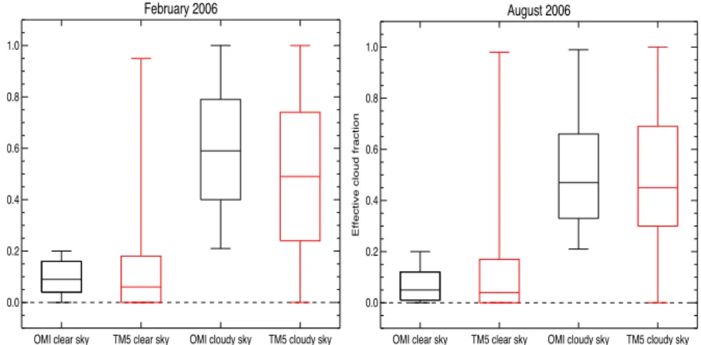
Figure 3 shows a box and whisker plot for OMI and TM5 effective cloud fractions over Europe in February and August 2006. The figure indicates that for OMI

mea-5

surements of effective cloud fractions smaller than 0.2, TM5 reproduces similar small effective cloud fractions (February median OMI: 0.09, TM5: 0.06; August median OMI: 0.05, TM5: 0.04). For days and locations when OMI observes e_ffective cloud fractions larger than 0.2 (February: 0.59, August: 0.47), TM5 simulates comparable high eff ec-tive cloud fractions (January: 0.49, July: 0.45), providing some confidence in the TM5

10

model, driven by ECMWF meteorological fields, to capture the observed e_ffective cloud fractions.

Figure 4a shows a comparison of average TM5 tropospheric NO₂columns simulated under clear-sky and cloudy situations over Europe in February and August 2006. TM5 was sampled for polluted situations (cells with monthly mean NO₂columns in excess of

15

1.0×1015molec cm−2) between 12:00–15:00 h local time, on days with clear skies and on days with cloud-cover. Under clear-sky situations, TM5 simulates tropospheric NO₂ columns that are on average 15–20 % lower than under cloudy circumstances, in line with in situ observations reported by Boersma et al. (2009) and Geddes et al. (2012) over Israeli and Canadian cities, respectively. Both in February and August, the

clear-20

sky mean NO₂column is 12 % below the 28 day monthly mean in February and 31 day monthly mean in August. Although we cannot rule out that other effects than enhanced photochemical loss may have contributed to lower NO₂columns over the polluted grid cells (e.g. increased ventilation or deposition) on clear-sky days, a comparison of NO₂ columns for all European grid cells showed that the geometrical mean of the local

clear-25

sky to cloudy column ratios was 0.74 in February and 0.89 in August, suggesting that reduced clear-sky NO₂columns presented in Fig. 4 show a robust e_ffect.

(23)

GMDD

8, 7821–7877, 2015

retrievals

Title Page

Tables Figures

◭ ◮

Back Close

Full Screen / Esc

Discussion

P

a

per

|

Discussion

P

a

per

|

Discussion

P

a

per

|

Discussion

P

a

per

|

higher under clear-sky situations than on cloudy days and the clear-sky mean HCHO column is 8 % higher than the all-sky monthly mean (August 2006). In winter, HCHO concentrations are generally low over Europe and differences between clear and cloudy sky are well below the detection limit of UV-Vis satellite sensors.

Exclusive sampling of the model on clear-sky days is important, because photolysis

5

rates J[NO₂] in the lower troposphere are significantly higher on those days and can be simulated well by TM5 (Williams et al., 2012), so that NO₂columns will be systemati-cally lower. The di_fferences between HCHO columns sampled on clear-sky and cloudy days are somewhat smaller than for NO₂columns because both the formation and de-struction of HCHO are driven by photochemistry. Nevertheless, the stronger

summer-10

time production of HCHO from the (OH-driven) oxidation of methane and especially isoprene outpaces the increased loss of HCHO through photolysis and oxidation (Fried et al., 1997) on clear-sky days compared to cloudy days, in line with observations (e.g. Munger et al., 1995; Cerquiera et al., 2003).

To estimate the magnitude of the temporal representativeness errors arising from

15

the particular choice of model sampling, we evaluated the satellite-model comparison results for di_fferent sampling strategies. Again, we use the averaged ratio of satel-lite measurements to model simulations ( ˆy_o/xˆ_m), and the spatio-temporal correlation coefficient, as appropriate indicators of representativeness errors. Since the model– measurement bias may well be due to unrelated systematic errors in either the CTM

20

(emissions, chemistry) or the satellite retrievals, we are not concerned with the abso-lute value of the measurement-to-model ratio, but we are interested in the sensitivity of the ratio to various sampling strategies. We tested four strategies for comparing tropo-spheric NO₂over large polluted regions: (A) both OMI (for OMI e_ffective cloud-fraction) and TM5 (TM5 effective cloud fraction) collocated and sampled for mostly clear-sky

25

scenes only at the OMI overpass time of 13:30 h, (B) OMI and TM5 collocated and

(24)

GMDD

8, 7821–7877, 2015

retrievals

Title Page

Tables Figures

◭ ◮

Back Close

Full Screen / Esc

Discussion

P

a

per

|

Discussion

P

a

per

|

Discussion

P

a

per

|

Discussion

P

a

per

|

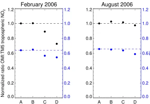
co-sampled for situations with OMI effective cloud radiance fractions <0.52, (C) OMI sampled for situations with OMI effective cloud radiance fractions<0.5, but TM5 more loosely sampled for OMI e_ffective cloud fractions<0.6, and (D) OMI sampled for situ-ations with OMI effective cloud radiance fractions<0.5, but TM5 sampled for all days in the month (i.e. no temporal collocation except for appropriate overpass time).

Strat-5

egy (A) is considered to be optimal, but to our knowledge has not been applied in studies to date. Strategy (B) has been followed in numerous studies, and relies on the assumption that CTMs capture the observed cloud cover well. In spite of its erro-neous co-sampling with the satellite measurements, strategy (D) has also been used frequently, and therefore we tested its impact on the temporal representativeness

er-10

rors. Finally, strategy (C) holds middle ground between (B) and (D). Figure 5 shows that the model-to-measurement ratio shows substantial dependence on the compari-son strategy, especially in Winter. The di_fferences between strategies (A) and (B) are negligible, but with strategy (D) the OMI/TM5 ratio drops more than 25 % below the val-ues obtained by strategies (A) and (B). These strategies also demonstrate that strategy

15

(D) leads to a reduced capacity of the model to explain the observed variability in the NO₂ spatial patterns, with R2 dropping almost 10 % (from 0.64 to 0.55 in Winter and from 0.66 to 0.59 in summer).

Analyses for other regions showed similar results as in Fig. 5. These results imply that for applications of satellite data such as emission estimates or model evaluations,

20

substantial systematic errors may occur in the final estimate, if sampling strategies such as (D) are used. We therefore strongly discourage the use of such comparison strategies, as they lead to considerable temporal representativeness errors, and, thus, systematic underestimations in measurement : model ratios.

2

(25)

GMDD

8, 7821–7877, 2015

retrievals

Title Page

Tables Figures

◭ ◮

Back Close

Full Screen / Esc

Discussion

P

a

per

|

Discussion

P

a

per

|

Discussion

P

a

per

|

Discussion

P

a

per

|

5.3 Vertical representativeness errors

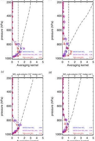
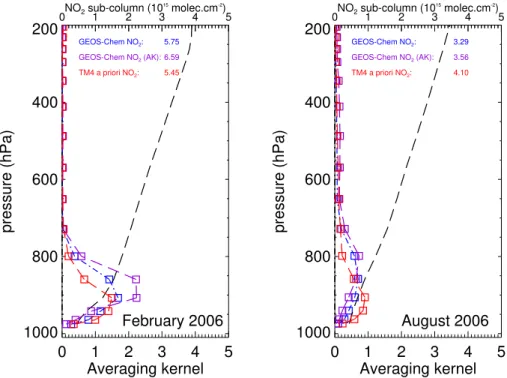
Here we evaluate the representativeness errors introduced in a satellite-model com-parison if the averaging kernel is not accounted for. To illustrate the way the kernels work, Fig. 6 shows GEOS-Chem NO₂ vertical profiles with and without the averaging kernel applied over the Beijing grid cell on clear-sky days with excellent spatial

cover-5

age (18 February and 23 August 2006). On both days, application of the kernel leads to a higher value for the model column, reflecting the relatively larger amounts of NO₂ aloft in GEOS-Chem simulations compared to the a priori TM4 NO₂profiles. The lower panels show that on two other clear-sky days (17 February and 31 August 2006) the kernel has only little effect on the GEOS-Chem tropospheric NO₂ column. On these

10

days, the TM4 a priori and GEOS-Chem NO₂ profiles show similar, less pronounced vertical distributions. Nevertheless, in Fig. 7 we see that, on average, for February and August 2006, the OMI averaging kernels result in increases in GEOS-Chem NO₂ columns over Beijing of 15 % (February) and 8 % (August), and a closer agreement with OMI NO₂retrievals. This result can be understood from the stronger vertical

mix-15

ing in the GEOS-Chem model compared to TM4, rather than from differences in NO_x emissions or chemistry between models (NO₂amounts are quite similar between TM4 and GEOS-Chem over Beijing in 2006).

The above finding does not have general validity in the sense that applying the kernel on any other model will also result in a tropospheric column increase. Applying the

20

kernels to NO₂profiles from a model with weaker vertical mixing than TM4 (rather than generally stronger vertical mixing as in the case of GEOS-Chem) is likely to reduce those columns. Figure S1 in the Supplement shows as much for the North Sea grid cell in February 2006, when GEOS-Chem exceeds TM4 NO₂ concentrations below 900 hPa, and for Siberia in August 2006, when GEOS-Chem simulates a substantially

25

enhanced tropospheric NO₂column compared to TM4.

We next compare the monthly averaged GEOS-Chem tropospheric NO₂ column fields for February and August 2006 with and without the kernels applied.

(26)

GMDD

8, 7821–7877, 2015

retrievals

Title Page

Tables Figures

◭ ◮

Back Close

Full Screen / Esc

Discussion

P

a

per

|

Discussion

P

a

per

|

Discussion

P

a

per

|

Discussion

P

a

per

|

ure 8 shows that applying the kernel leads to substantial increases of up to 2×

1015molec cm−2 in the columns for the polluted source regions in the Northern Hemi-sphere (eastern USA, Europe, and China). At the periphery of these regions in win-tertime, and over regions with possible biomass burning in summer, we see that the smoothed columns can be lower than the original columns, indicating that the

GEOS-5

Chem vertical NO₂profile is more skewed towards the surface than the TM4 a priori in those situations, as confirmed by the profiles shown in Fig. S1.

Here we evaluate the level of agreement between the original GEOS-Chem and OMI NO₂ columns, compared to the level of agreement between the kernel-based GEOS-Chem and OMI NO₂ column for the polluted source regions in the Northern

Hemi-10

sphere, as the di_fferences provide a measure of the representativeness errors that can be avoided by using the averaging kernel. Figure 9 shows the agreement between OMI and the GEOS-Chem NO₂columns with and without kernel over Europe in Febru-ary and August 2006. The upper panels indicate that the spatial correlation between the model and OMI tropospheric columns improves when the kernel is applied on the

15

model NO₂profiles, especially in summer when differences between the TM4 a priori and GEOS-Chem NO₂profile shapes are strong. Application of the kernel also results in geometric mean OMI : GEOS-Chem ratios with smaller uncertainty intervals at val-ues of 1.151.82_0.73(February) and 1.241.78_0.86(August) compared to 1.131.82_0.70and 1.422.14_0.94. We find similar results over the eastern United States and China (see Table 1 in Sect. 7).

20

Figure 9d further supports the notion that application of the kernel allows for a better-constrained evaluation of the model, as witnessed by the more peaked and narrower histogram of satellite : model ratios. We conclude that sampling the model according to the averaging kernel is especially relevant in summer, and improves the satellite-model evaluation by removing differences between (TM4 apriori and GEOS-chem) profile

25

(27)

GMDD

8, 7821–7877, 2015

retrievals

Title Page

Tables Figures

◭ ◮

Back Close

Full Screen / Esc

Discussion

P

a

per

|

Discussion

P

a

per

|

Discussion

P

a

per

|

Discussion

P

a

per

|

6 Combined representativeness errors

To obtain an estimate of typical, overall representativeness errors in model evaluations with UV/Vis satellite measurements, we define three types of model evaluations, exe-cuted with increasing degree of detail. We again evaluate tropospheric NO₂ from the GEOS-Chem model here (with OMI NO₂ retrievals), as this model is su_fficiently di_ff

er-5

ent from the TM4 model used to provide the a priori profiles in the OMI retrievals. The three types of evaluations can be characterised as advanced, common, and naïve:

(A) advanced evaluation: accounting for su_fficient spatial coverage and appropriate temporal representativeness, and also taking into account vertical representative-ness,

10

(B) common evaluation: as (A) but without taking into account vertical sensitivity,

(C) naïve evaluation: no consideration of potential representativeness errors whatso-ever,

For evaluation (C), the model monthly average was based on samples from all days of the month (on OMI overpass time), irrespective of cloud coverage, and no kernel was

15

applied (in other words a 31-day, all-sky, without AK monthly mean). We first evaluate the (avoidable) representativeness errors by comparing local OMI : GEOS-Chem ratios evaluated with approaches (A) vs. (C), and approaches (A) vs. (B). Figure 10 shows the relative difference in the local OMI : GEOS-Chem ratios for February and August 2006. We see that the systematic, avoidable errors in the OMI : GEOS-Chem ratio are largest

20

with evaluation approach (C). The blue colours in the upper panel of Fig. 10a indicate that, in winter, sampling the model on all (including cloudy sky) days leads to too low (by 15–20 %) OMI/GEOS-Chem ratios reflecting the too high GEOS-Chem NO₂ values resulting from temporal representativeness errors (cloudy-sky sampling cf. Fig. 4).

The similarity between the panels of Fig. 10b shows that appropriate sampling is

25

not as important in summer, a season with ample clear-sky days, and, consequently, a smaller sampling error. Figure 10b suggests that application of the averaging kernel