Amplitude Amplification Factor of Bi-chromatic
Waves Propagation in Hydrodynamic Laboratories
Marwan Ramli
Abstract—This paper focuses on peaking and splitting phe-nomena of waves, in order to support hydrodynamic laboratory activities for generating waves which have large amplitude and are very steep but do not break during their propagation in the wave tank. Such waves, called extreme waves or giant waves, will be used to test oceanic objects, like ships and marine structures, before they operate in real condition. The previous study shows that nonlinear effects will deform the initial wave and may lead to large waves with height larger than twice as high as the original input; the deformation is followed by peaking and splitting phenomena. It is interesting to understand and quantify the nonlinear effects; it is also interesting to know at which location in the wave tank, the extreme position, the waves will achieve their maximum amplitude and how high the magnitude of the amplitude at this position. As in the previous research, a quantity that can be used to investigate these phenomena is Maximal Temporal Amplitude (MTA). MTA can be used to measure the maximum amplitude amplification of the wave elevation at each location during the observation time. It is known that an explicit expression of the MTA can not be found in the general form of the governing equations (the full Euler equations with the exact kinematic and dynamic free surface conditions) and generating signals. Simplified models, like Boussinesq, Korteweg de Vries (KdV) and Non Linear Schrodinger (NLS) type of equations which have in common that the fluid motion in the layer is approximated to arrive at equations at the free surface alone are considered. By using the third order approximation of KdV (TOA-KdV) or Boussinesq (TOA-Bouss) and MTA, it is obtained a formula that can be used to predict the extreme position. Furthermore, the fifth order approximation of KdV (FOA-KdV) and MTA is used to investigate the amplitude amplification, and the order of amplitude amplification factor (AAF) is obtained. TheAAF
here is the ratio of the amplitude at maximum location to the initial amplitude. However, theAAF which is calculated using FOA-KdV does not match the experimental results. Therefore, in this paper we use Boussinesq model with full dispersion and the same method and procedure with the previous research. Furthermore, we verify our theoretical results using analytical and numerical as well as experimental results.
Index Terms—Boussinesq equation, MTA, bi-chromatic waves, wave propagation, asymptotic expansion, amplitude amplification factor.
I. INTRODUCTION
T
HIS paper concerns on peaking and splitting phenom-ena of waves during their propagation in hydrodynamic laboratory. It is directly motivated by the need to generate waves with high and steep amplitude, called extreme waves, but not break during their propagation in the wave basin in hydrodynamic laboratory. Such waves will be used to test a floating body before it operates in real situation. The extremeManuscript received March 25, 2015; revised November 17, 2015. This research is funded by Syiah Kuala University, Ministry of Education and Culture Republic of Indonesia through Competency Research 2015, Contract Number : 035/SP2H/PL/Dit.Litabmas/II/2015 dated l5 February 2015
Marwan Ramli, Department of Mathematics, Syiah Kuala University, Banda Aceh, 23111, Indonesia. E-mail: [email protected] or [email protected].
wave is a wave whose height exceeds the significant wave height of measured wave train by factor more than 2.2 [1] and [2]. Occurrences (where and when) of this wave are not easy to predict, but its impact can cause damage to oceanic objects, i.e. ships and marine structures, that are around this wave (see Earle [3], Mori et al [4], Divinsky and Levin [5], Truslen and Dysthe [6], Smith [7], Toffoli and Bitner [8] and Waseda et al. [9]). Therefore, information about the presence of freak waves is important for offshore activities. The presence has been often reported in media. Nikolkina and Didenkulova [10] collected and analysed freak waves reported in media in 2006-2010. To understand the occurrence, propagation and generation of the extreme wave, various studies have been conducted by many researchers. Waseda et al. [11] conducted deep water observation of freak waves in the North West Pacific Ocean. Hu et al. [12] studied numerically rogue wave based on nonlinear Schrodinger breather solutions under finite water depth. Islas and Schober [13] investigated the effects of dissipation on the development of rogue waves and down shifting by adding nonlinear and linear damping terms to the one-dimensional Dysthe equation. Xu et al. [14] proposed (2 + 1)- dimensional Kadomtsev–Petviashvili equation, homoclinic (heteroclinic) breather limit method (HBLM), for seeking rogue wave solu-tion to nonlinear evolusolu-tion equasolu-tion (NEE). The wave ampli-fication in the framework of forced non linear Schrodinger equation is observed by Slunyaev et al. [15]. Cahyono et al. [16] discussed multi-parameters perturbation method for dispersive and nonlinear partial differential equations. Ramli [17] investigated nonlinear evolution of wave group with three frequencies using third order approximation of Ko-rteweg de Vries equation and Maximal Temporal Amplitude. Wabnitz et al. [18] observed extreme wave events which are generated in the modulationally stable normal dispersion regime. Peric et al. [19] regarded a prototype for spatio-temporally localizing rogue waves on the ocean caused by nonlinear focusing and analyzed by direct numerical simulations based on two phase Navier–Stokes equations. Blackledge [20] found the explicit freak waves can not be obtained by pure intuition or by elementary calculations because of their complications. Onorato et al. [21] discussed rogue waves occurring in different physical contexts and related anomalous statistics of the wave amplitude, which deviates from the Gaussian behavior that were expected for random waves. Extreme wave generation using self-correcting method was studied by Fernandez et al. [22]. Xi-eng et al. [23] simulated the extreme wave generation are carried out by using the volume of fluid (VOF) method.
the wave tank. As effects of non-linearity the original signal will deform during its propagation, (see[24], [25], [26] and [27]). The deformation, which is followed by peaking and splitting phenomena, may lead to amplitude amplification of the waves so that waves can occur with wave height that can not be generated in a direct way by wave-maker motions [28]. Due to physical limitations of the wave generator, the nonlinear effects are very difficult to study over the long distance and time that are relevant for the laboratory [29].
In order to support the extreme wave generation activity in hydrodynamic laboratory, Marwan et al. [30], [31] and [32] found the formula to predict the position at which bi-chromatic and Benjamin-Feir waves will reach maximum during their propagation. Such formula is derived based on the third order approximation of KdV equation (TOA-KdV). Based on the formula the position where bi-chromatic waves reach highest peaking of order (1
a2,ν12), with a and
ν are the initial amplitude and the envelope frequency, respectively. Obtained results with that approximation in accordance with the results of Stansbergs experiment [25] and Westhuis numerical study [26] and [27], are described in Marwan [31]. However, although it can predict the position, the third-order approximation of KdV equation is not able to be used to predict an increase of either bi-chromatic or Benjamin-Feir wave amplitude (see Marwan [31], [32] and [33]). In the other word, obtained results do not appropriate with the Stansbergs experimental results [25] and Westhuis numerical study [26] to predict an increase of bi-chromatic wave amplitude. However, this incompatibility was expected in the first place because the calculation is done up to the third-order only. Therefore, different from [21], [22] and [23], Ramli et al. [34] studied bi-chromatic wave propagation with fifth-order of KdV equation (FOA-KdV) and MTA. Obtained results show that there is an increase in the related bi-chromatic wave amplitude as high order influence, and the increasing of the amplitude is of order (a
ν)
2.
Never-theless, the increasing is still not suitable with Stansberg’s experimental result [25] and Westhuis’s numerical study [26]. It should be stated that the KdV equation in conducted study is KdV equation with exact dispersion relation found by Groesen [35]. For this fact, in this paper we will use Boussinesq model with full dispersion and MTA by using the same procedure as in [36] to investigate the amplitude amplification factor (AAF) for increasing amplitude of bi-chromatic waves in their propagation. It is known that from this model, it can be derived KdV equation through uni-directionalization process (see [37], [38] and [39]). As it is what has been shown in previous work, see also [40], for narrow banded spectra, the third order effects can dominate the second order effects and are responsible for the large amplification factor. For that reason we also use third order theory for our analysis.
The organization of the paper is as follows. In the next section we present the mathematical model to be used, the third order side band solution for this model and the approximation of the amplitude amplification factor by an explicit expression obtained from third order side band. Some graphical results and the comparison with the previous results of the amplitude amplification factor are presented in Section 3. Finally in Section 4, we make some concluding remarks.
II. AMPLITUDEAMPLIFICATIONFACTOR
As mentioned above, as an effect of non-linearity the surface waves deform. This deformation is followed by splitting and peaking phenomena, during their propagation in hydrodynamic laboratory. To investigate this directly through the full Euler equations with the exact kinematic and dynamic free surface conditions is not easy. Simplified models, like Boussinesq, Korteweg de Vries (KdV) and Non Linear Schrodinger (NLS) type of equations which have in common that the fluid motion in the layer is approximated to arrive at equations at the free surface alone are considered. In this article we use Boussinesq equation as a model. The Boussinesq equation is known as an asymptotic model for two opposite directional rather long and small wave that propagates on the surface. In normalized variables, the Boussinesq equation with full dispersion [35] has the form
∂tu+∂xη+u∂xu= 0
∂tη+∂x(Lu) +∂x(uη) = 0, (1)
with u and η are velocity and elevation of the wave in normalized coordinate, respectively. Here, L is pseudo-differential operator with Fourier symbol
b
L(k) =tanhk
k .
The laboratory variables for the wave elevation, velocity, horizontal space and timeηlab,ulab,xlabandtlabare related
to the normalized variables by ηlab = hη, ulab = u√gh,
xlab = hx and tlab = t
p
h/g, where h is the uniform water depth andg is the gravity acceleration. Consequently, corresponding transformed wave parameters such as wave length, wave number and angular frequency, are given by λlab=hλ, klab=k/h, ωlab=ω
p g/h.
As it is in [16], [36] and different from Huang [41], in this paper the solution of (1) is obtained by using a direct expansion up to third order in the power series of the wave elevation and velocity. Here, we write
η=ε η(1)+ε2η(2)+ε3η(3)+
O(ε4)
u=ε u(1)+ε2u(2)+ε3u(3)+O(ε4), (2)
whereεis a positive small number representing the order of magnitude of the wave amplitude. The terms η(j) andu(j)
describe the solution of elevation and velocity at jth
order, j= 1,2,3, respectively. It is known that this direct expansion leads to resonance in the third order, see [39], [40], [42]. To avoid this resonance, a modification is introduced. The modification used is the development of Linstead-Poincare technique [43] which produces nonlinear dispersion relation [39]
k± ≈k
(0)
± +εk
(1)
± +ε2k
(2)
± (3)
with
ω± =k
(0)
± q
b
L(k±(0)). (4)
Since this paper focuses on bi-chromatic waves, hereη(1)
is chosen as
η(1)= 4acos(θ) cos(∆θ), (5)
with
and
∆θ= θ+−θ−
2 ,
θ±=k±x−ω±t,(k±, ω±)satisfies the nonlinear dispersion relation. As reported in [36], at the second order it is obtained the following forms
k(1)± = 0,
η(2)(x, t) =s+cos 2θ++s−cos 2θ−+scos 2θ+smcos 2∆θ, (6) and
ηf w(2)(x, t) = s+cosϑ(2ω+) +s−cosϑ(2ω−)
+scosϑ(2ω) +smcosϑ(2ν), (7) withϑ(ω) = Ω−1(ω)x
−ωt. The coefficients s±,sandsm in equation (6) are given by
s± = 2k
(0)
± (2ω±2 +L(2k
(0)
± )) ω2
±(2ω±+ 2k
(0)
± L(2k
(0)
± ))
a2k(0)
±
2ω±−2k
(0)
± L(2k
(0)
± ) ,
s= klin
2
a(b−+b+)ω+b+b−klinL(2klin)
(ω)2−(k
lin)2L(2klin)
,
sm= κlin
2
a(b−+b+)ν+b+b−κlinL(2κlin)
ν2−(κ
lin)2L(2κlin)
,
withb±=
ak(0)±
ω± ,klin =
1 2(k
(0) + +k
(0)
− )andκlin= 12(k
(0) + −
k(0)− ).
Then, at the third order, it successively produces [36]
k(2)± = −
ω±(b±s±+b∓s+b∓sm+aB±+aB+aBm)
a(2L(k(0)± ) +k
(0)
± L′(k
(0)
± ))
−k
(0)
± L(k
(0)
± )(b±B±+b∓B+b∓Bm)
a(2L(k±(0)) +k±(0)L′(k(0) ± ))
, (8)
ηsb(3)(x, t) =A+3cos(θ+ 3∆θ) +A−3cos(θ−3∆θ), (9) and
η(3)sb,f w(x, t) =A+3cosϑ(ω+ 3ν) +A−3cosϑ(ω−3ν),
(10) with B± =
k(0)±
2ω±(b
2
±+ 2s±), B= klinω (s+b+b−),Bm= κlin
ν (sm+b+b−).
For ν → 0 implies κlin → 0 gives sm → σ0, Bm →
1
Ω′(K(ω))σ0,s,s± → σ2andB, B± →
K(ω)
ω σ2(see [35]),
with
σ0=
1
Ω′(K(ω))−1, σ2=
K(ω) 2ω−Ω(2K(ω)),
K= Ω−1(ω),Ω(k) =k r
tanhk k . The coefficientsA±3 in (9) and (10) are given by
A±3 =
(klin±3κlin)L(klin±3κlin)(b∓B±+b±Bm)
+(ω±3ν)(b∓s±+b±sm+a(B±+Bm))
klin±3κlin
(ω±3ν)2−(k
lin±3κlin)2L(klin±3κlin)
.
Observe that forν → 0, these coefficients can be expressed as
A±3≈ a
3(σ 0+σ2)
2κ2
linΩ′′(k
(0)
± )± 43κ3linΩ′′′(k
(0)
± ) .
It implies the equation (9) and (10) can also be written as
ηsb(3)(x, t) =a
a κlin
2
[m+cosθcos 3∆θ−m−sinθsin 3∆θ]
(11)
ηsb,f w(3) (x, t) =a
a κlin
2
[m+cosKcosKe−m−3sinKsinKe],
(12) with
m+ ≈ −
σ0+σ2 Ω′′(k(0)
± )
, m−≈
(σ0+σ2)Ω′′′(k±(0))
(Ω′′(k(0) ± ))2
κlin,
K= K(ω+ 3ν) +K(ω−3ν) 2
and
e
K= K(ω+ 3ν)−K(ω−3ν)
2 .
As reported in [24], [25], [26] and [27], it was found ex-perimentally, numerically, and theoretically that bi-chromatic waves deform during their propagation. The deformation is followed by peaking and splitting phenomena. It is known that the peaking phenomena does not only depend on the wave amplitude, but also depend on the frequency difference of monochromatic components of the bi-chromatic waves. Marwan and Andonowati [42] introduced a quantity called the MTA which has been used also for optical problems [40] to observe the phenomena. The scale used to measure the height of the wave at each position is defined as [42]
m(x) = max
t η(x, t), t >0. (13)
The MTA (13) can be used to predict the position at which the waves will reach the highest peaking during their propagation in the wave tank [31]. To know the wave elevation changes, the ratio of the highest value of MTA to the value of MTA at the wave maker is observed and called as the amplitude amplification factor (AAF), which is defined as [32]
AAF =m(xmax)
m(0) , (14)
where xmax is the first position where m(xmax) = maxxm(x), for 0 < x < Lˆ and Lˆ is the length of the
wave tank.
As mentioned above, this paper focuses only on the term that have the greatest contribution in each order, then the solution of equation (1) that satisfies the boundary conditions in a bi-chromatic signals at wave maker can be written as
η=η(1)+η(2)−ηf w(2)+η(3)sb −ηsb,f w(3) , (15) namely the third order approximation of Boussinesq equation (TOA-Bouss). Substituting the expressions of (5), (11) and (12) into (15), and using the assumption that contribution of the second order smaller than the other order, give
η(−2) = 4acos(θ) cos(∆θ) + 4a
a κlin
2
m+cosθ
cos 3∆θ−4a
a κlin
2
m+cosKcosK.e (16)
orderO
1 + a κlin
2
as reported in [34] for bi-chormatic waves which are calculated using FOA-KdV equation.
III. RESULT ANDDISCUSSION
In this section some graphical results are presented. All values in this calculations are given in the laboratory coor-dinate systems [m,kg,s]. Here we use the same example for bi-chromatic case as in Ramli et al [34].
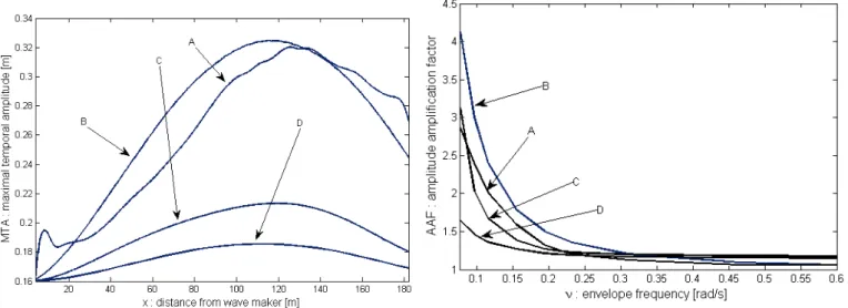
The MTA of the waves as a function of the spatial variable x, 0 ≤ x ≤ 180 m, is plotted in Figure 1. In fact, in this figure, there are four plots : the MTA of experimental result as well as HUBRIS software (A), the third order approximation of Boussinesq equation (TOA-Bouss)(m(−2)(x) = maxtη(−2)(x, t))(B), the fifth order
approximation of KdV equation (FOA-KdV)(C) and the third order approximation of KdV equation (TOA-KdV) (D). It can be seen that the location of MTA reaching the maximum from all of the four approximations are quite similar. Furthermore it can also be seen that the maximum value of MTA which was calculated using TOA-Bouss equation (B) matches the numerical software HUBRIS result (A).
Fig. 1. Plot of MTA as a function ofx,0≤x≤180m, witha= 0.04
m,ω= 3,145rad/s andν= 0,155rad/s. Computation using numerical software HUBRIS (A)[27], calculations using TOA-Bouss(m(−2)(x) =
maxtη(
−2)(x, t)) (B) [36], calculation using FOA-KdV (C) [34] and
calculation using TOA-KdV (D) [31], [32]. It shows the conformity of location MTA reaching the maximum from all of the four approaches. Beside that, it can be seen that the maximum value of MTA which is calculated using TOA-Bouss is suitable with the maximum value of MTA which is calculated using numerical software HUBRIS.
In Figure 2 we plot the AAF of the bi-chromatic waves as a function of wave amplitude (a) forω= 3,145rad/s and ν = 0,155 rad/s. It shows that increasing value ofahas an effect on increasing value of AAF. This is in accordance with the formula derived in Section 3 that the AAF is of order O( 1 +a2) for constant ν. From this figure, it
can also be seen that AAFs which are calculated using all of the four approximations have the same dependence on a. Furthermore, from the figure it can be seen that AAF which is calculated using TOA-Bouss (B) agrees the AAF which is calculated using numerical software HUBRIS (A). Meanwhile, theAAFs which are calculated using FOA-KdV (C) and TOA-KdV (D) are smaller than the AAF which is calculated using numerical software HUBRIS (A). The
Fig. 2. Plot ofAAF (14) as a function of wave amplitude (a),0.005≤ a≤0.045m, withω= 3,145rad/s andν= 0,155rad/s. Computation using numerical Software HUBRIS (A) [27], calculation using TOA-Bouss (B) [36], calculation using FOA-KdV (C) [34] and calculations using TOA-KdV (D) [31], [32]. It is shows that the AAFs of bi-chromatic waves which are calculated using all these the four approximations have the same dependence ona.
Fig. 3. Plot ofAAF(14) as a function of envelope frequency (ν),0.075≤ ν ≤ 0.6rad/s, withω = 3,145 rad/s anda = 0,035m. Computation using numerical Software HUBRIS (A)[27], calculation using TOA-Bouss (B) [36], calculation using FOA-KdV (C) [34] and calculations using TOA-KdV (D) [31], [32]. It is shows that the AAFs of bi-chromatic waves which are calculated using all these the four approximations have the same dependence onν.
similar thing can also be seen in Figure 3. Figure 3 presents the plot ofAAF as a function of envelope frequency(ν) for ω = 3,145 rad/s and a = 0,035 m. In this figure we can see that increasing value ofνaffects on decreasing ofAAF. From this figure, it can also be seen that AAFs which are calculated using all of the four approximations have the same dependence onν.
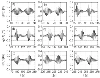
In Figure 4 and Figure 5, we present signals at some locations in the wave tank which are calculated using TOA-Bouss and numerical software HUBRIS, respectively, for an input bi-chromatics signals with a = 0.04 m, ω = 3,145
distance is the extreme position. From both figures, it can be seen that the bi-chromatic signals at given location which are calculated using TOA-Bouss have quite similar shape with the bi-chromatic signals which are computed using numerical software HUBRIS [27] as well as experimental result [25].
Fig. 4. Bi-chromatic signals at some positions (15) for a = 0.04 m,
ω = 3.145rad/s and ν = 0.155rad/s which are calculated using TOA-Bouss. Bi-chromatic signals at position : a)x= 0, b)x= 53m, c)x= 93
m, d)x= 120m, e)x= 153m, f)x= 173m, g)x= 193m, h)x= 213
m, i)x= 233m
Fig. 5. Bi-chromatic signals at some positions fora= 0.04m,ω= 3.145
rad/s andν = 0.155rad/s which are computed using numerical software HUBRIS. Bi-chromatic signals at position : a) x= 0, b)x= 53m, c)
x= 93m, d)x= 120m, e)x= 153m, f)x= 173m, g)x= 193m, h)x= 213m, i)x= 233m.
IV. CONCLUDINGREMARKS
Bi-chromatic waves propagation in hydrodynamic labora-tory are considered. The waves contain signals which have two mono-chromatic components with the same amplitudes but slightly different of frequencies. During their propagation in the wave tank, the waves deform and it is followed by splitting and peaking phenomena (amplitude increasing). To find the amplitude amplification factor (AAF) of the waves in the tank, the concept of MTA for third order approximation of Boussinesq equation has been used. MTA
gives at each location in the wave tank the maximum value of the surface elevation over time andAAF.
We have verified the calculated formula forAAF with the published numerical result. This comparisons show reason-ably close values of the predicted amplitude amplification factor of the waves to the known results.
ACKNOWLEDGMENT
The author is very grateful Dr. J. H. Westhuis for making HUBRIS accessible to verify the results of this paper. Also the author sincerely thank to Said Munzir, T. Khairuman and Vera Halfiani for fruitful discussion throughout the execution of this research
REFERENCES
[1] R.G. Dean, ”Freak waves : a possible explanation”, Water Wave Kinetics,Kluwer, Amsterdam, pp. 609-621, 1990
[2] S.P. Kjeldsen, ”Dangerous wave group”,Norwegian Maritime Research, vol. 12, pp. 16, 1984
[3] M.D. Earle, ”Extreme wave conditions during hurricane Camille”,J. Geophys. Res, vol. 80, pp. 377-379, 1975
[4] N. Mori, P. C. Liu and T. Yasuda, ”Analysis of freak wave measure-ments in the sea of Japan”,Ocean Eng., vol. 29, pp. 1399-1414, 2002 [5] B. V. Divinsky, B. V. Levin, L. I. Lopatikin, E. N. Pelinovsky and A. V. Slyungaev, ”A freak wave in the Black Sea, observations and simulation”,Doklady Earth Sci., vol. 395, pp. 438-443, 2004 [6] K. Trulsen and K. Dysthe, ”Freak waves a three dimensional wave
simulation”,Proc. of the 21st Symposium on Naval Hydrodynamics, E. P. Rood, ed., National Academy Press, pp. 550-558, 1997
[7] R. Smith, ”Giant waves”,J. Fluid Mech., vol. 77, pp. 417-431, 1976 [8] E. M. Toffoli and B. Gregersen, ”Extreme and rogue waves in
direc-tional wave fields”,The Open Ocean Eng. J., vol. 4, pp. 24-33, 2001 [9] T. Waseda, H. Tamura, T. Kinoshita, ”Freakish sea index and sea states
during ship accidents”,J. Marine Sci. Tech., vol. 17, pp. 305-314, 2012 [10] I. Nikolkina and I. Didenkulova, ”Catalogue of rogue waves reported in media in 2006-2010”,Nat. Hazards, vol. 61, pp. 989-1006, 2012 [11] T. Waseda, M. Sinchi, K. Kiyomatsu, T. Nishida, S. Takahashi,
S. Asaumi, Y. Kawai, H. Tamura and Y. Miyazawa, ”Deep water observations of extreme waves with moored and free GPS buoys”,
Ocean Dyn., vol. 64, pp. 1269-1280, 2014
[12] Z. Hu, W. Tang, H. Xu, X. Zhang, ”Numerical study of rogue waves as non linear Schrodinger breather solutions un-der finite water depth”, Wave Motion, vol. 52, pp. 81-90, 2015, http://dx.doi.org/10.1016/j.wavemoti.2014.09.002
[13] A. Islas, C.M. Schober, ”Rogue waves, dissipation, and down shifting”, Phys., vol. 240, pp. 1041-1054, 2011, http://dx.doi.org/10.1016/j.physd.2011.03.002
[14] Z. Xu, H. Chen, Z. Da, ”Rogue wave for the (2 + 1)-dimensional KadomtsevPetviashvili equation”,App. Math. Let., vol. 37, pp. 34-38, 2014, http://dx.doi.org/10.1016/j.aml.2014.05.005
[15] A. Slunyaev, A. Sergeeva, E. Pelinovsky, ”Wave amplification in the framework of forced non linear Schrodinger equation: the rogue wave context”, Phys. D, vol. 303, pp. 18-27, 2015, http://dx.doi.org/10.1016/j.physd.2015.03.004
[16] E. Cahyono, L.O. Ngkoimani and M. Ramli, ”Multi-parameters Per-turbation Method for Dispersive and Nonlinear Partial Differential Equations”,Int. J. Math. Anal, vol. 97, no. 43, pp. 2121-2132, 2015, http://dx.doi.org/10.12988/ijma.2015.56158
[17] M. Ramli, ”Non linear evolution of wave group with three frequen-cies”, Far East J. Math. Sci., vol. 97, no. 8, pp. 925-937, 2015, http://dx.doi.org/10.17654/FJMSAug2015 925 937
[18] S. Wabnitz, C. Finot, J. Fatomeb, G. Millot, ”Shallow water rogue wave trains in non linear optical fibers”, Phys. Let. A, vol. 377, pp. 932-939, 2013, http://dx.doi.org/10.1016/j.physleta.2013.02.007 [19] R. Peric, N. Hoffmannb, A. Chabchoubd, ”Initial wave breaking
dynamics of Peregrine-type rogue waves: a numerical and experi-mental study”, Eur. J. Mech. B Fluids, vol. 49, pp. 71-76, 2015, http://dx.doi.org/10.1016/j.euromechflu.2014.07.002
[20] J. M. Blackledge, ”A generalized non linear model for the evolution of low frequency freak waves”,IAENG Int. J. App. Math., vol. 41, no. 1, pp. 33-55, 2011
[22] H. Fernandez, V. Sriramb, S. Schimmels, H. Oumeraci, ”Extreme wave generation using self correcting method revisited”,Coastal Eng., vol. 93, pp. 15-31, 2014, http://dx.doi.org/10.1016/j.coastaleng.2014.07.003 [23] Z.Xi-zeng, H.C-hong, S.Z-chen, ”Numerical simulation of extreme wave generation using VOF method”,J. Hyd., vol. 22, No. 4, pp. 466-477, 2010, http://dx.doi.org/10.1016/S1001-6058(09)60078-0 [24] E. van Groesen, Andonowati, E. Soewono, ”Non linear effects in
bi-chromatic rurface waves”,Proc. Estonian Acad. Sci. Math. Phys., vol. 48, pp. 206-229, 1999
[25] C.T. Stansberg, ”On the non linear behaviour of ocean wave groups”,
Ocean Wave Measurement and Analysis, Reston, VA, USA : American Society of Civil Engineers (ASCE), vol. 2, pp. 1127-1241, 1998 [26] J. Westhuis, E. van Groesen, R. Huijsmans, ”Long time evolution
of unstable bi-chromatic waves”,Proc. 15th IWWW&FB, Caesarea Israel, pp. 184-187, 2000
[27] J. Westhuis, E. van Groesen, R. Huijsmans, ”Experiments and numer-ics of bi-chromatic wave groups”,J. Waterway Port Coast. Ocean Eng., vol. 127, pp. 334-342, 2000
[28] Andonowati, N. Karjanto, E. van Groesen, ”Extreme waves phenom-ena in down-stream running modulated”,App. Math. Mod., vol. 31, no. 7, pp. 1425-1443, 2007
[29] E. van Groesen, F.S. Widoyono and T. Nusantara, ”Modelling waves in a Towing Tank”,J. Indones. Math. Soc., vol. 4, pp. 55-68, 1998 [30] Marwan, Surface water waves: theory, numerics, and its applications
on the generation of extreme waves, Ph.D Thesis, Fac. of Mathematical and Sciences Institut Teknologi Bandung, Indonesia, 2006.
[31] Marwan, ”On the predicting extreme location and amplification of downstream propagation of bi-chromatic wave groups in hydrodynamic laboratory”,J. Dinamika Teknik Sipil, vol. 10, no.1, pp. 96-101, 2010 [32] Marwan, ”On the maximal temporal amplitude of down stream running
non linear water waves”,Tamkang J. Math., vol. 40, no. 1, pp. 51-69, 2010
[33] M. Ramli, ”The deterministic generation of extreme surface water waves based on soliton on finite background in laboratory”,Int. J. Eng, vol. 22, no. 3, pp. 243-249, 2009
[34] M. Ramli, S. Munzir, T. Khairuman, V. Halfiani, ”Amplitude increas-ing formula of bichromatic wave propagation based on fifth order side band solution of Korteweg de Vries equation”,Far East J. Math. Sci, vol. 93, no. 1, pp. 97-117, 2014
[35] E. van Groesen, ”Wave groups in uni-directional surface wave mod-els”,J. Eng. Math., vol. 34, pp. 215-226, 1998
[36] Marwan and Andonowati, ”The extreme position and amplitude ampli-fication of bichromatic waves propagation based on third order solution of Boussinesq equations”,J. Indones. Math. Soc., vol. 14, no. 2, pp. 95-110, 2008
[37] F.P.H. van Beckum, Hamiltonian consistent discretisation of wave equations, PhD thesis, University of Twente, The Netherlands, 1995 [38] S.R. Pudjaprasetya, Evolution of waves above slightly varying bottom:
a variational approach, PhD thesis, University of Twente, The Nether-lands, 1996
[39] E. Cahyono, Analytical wave codes for predicting surface waves in a Laboratory Basin, Ph.D Thesis, Fac. of Mathematical Sciences Univ. of Twente, the Netherlands, 2002
[40] Andonowati and E. van Groesen, ”Optical pulse deformation in second order non linear media”,J. Non-linear Opt. Phys. Materials, vol. 12, no. 22, pp. 221-234, 2003
[41] Y. Huang, ”Explicit multi-soliton solutions for the KdV equation by Darboux Transformation”,IAENG Int. J. App. Math., vol. 43, no. 3, pp. 135-137, 2013
[42] Marwan and Andonowati, ”Wave deformation on the propagation of bi-chromatics signal and its effect to the maximum amplitude”,J. Math. Sci., vol. 8, no. 2, pp. 81-87, 2003