DOI: http://dx.doi.org/10.1590/1806-9126-RBEF-2018-0236 Licença Creative Commons
On the Counterpropagation of Waves
Roger Pizzato Nunes
∗1, Gunther J. L. Gerhardt
2, Felipe Barbedo Rizzato
31Universidade Federal do Rio Grande do Sul, Departamento de Engenharia Elétrica, Escola de Engenharia, RS, Brasil 2Universidade de Caxias do Sul, Departamento de Física e Química, Centro de Ciências Exatas e Tecnologia, Caxias do Sul,
RS, Brasil
3Universidade Federal do Rio Grande do Sul, Instituto de Fisica, Porto Alegre, RS, Brasil
Received on August 14, 2018; Revised on September 02, 2018; Accepted on September 04, 2018. This work analyses the counterpropagation of transversal plane waves in a linear, homogeneous, nondispersive, and isotropic medium. Although this is a traditional subject in disciplines associated with wave phenomena, a propagation analysis is not found in the literature. With this purpose, the resultant wave and consecutively its phase velocity in such system are obtained analytically. Instead of what happens with the individual waves, the analytical results demonstrate that the phase velocity of the resultant wave actually is not a constant and depends explicitly of the time or the spatial coordinates, and principally depends of the amplitudes of the individual waves. This last remarkable feature, when considering as example electromagnetic systems, can be used to adequately control and accelerate particles in a charged medium. Full agreement between the analytical and numerical results is found.
Keywords:waves, propagation, phase velocity
1. Introduction
The known physics can be essentially reduced and divided in two branches: one associated with particle phenomena and the other involving wave phenomena. The wave phe-nomena permeate many areas of physics such as mechan-ics, thermodynammechan-ics, electromagnetism, relativity, and quantum mechanics. One important theme associated with wave phenomena is propagation [1,2]. Essentially, wave propagation can be affected by the changing of the physical medium properties (for example, in elec-trodynamics the electrical permittivityǫ, the magnetic permeability µ, among others), by the changing of the physical medium geometry (the changing in boundaries or the inclusion of another, as obstacles), by the existence of another waves, or by the existence of the matter. [3] Understanding how a wave propagates in a given system is of fundamental importance to understand the physics it represents.
Every propagation analysis initiates obtaining what it is called the wave vectorβfor a given angular frequency
ωin a given physical system. Technically, the propagation analyses initiates with the determination of the dispersion relationω(β)of the waves in the physical system. Once the dispersion relation is obtained, it becomes relevant to know how fast the wave propagates in the physical system. In other words, it is necessary to determine the velocity of the waves in the physical system.
One typical problem involving wave propagation is the case of waves propagating in opposite directions in
∗Endereço de correspondência: [email protected].
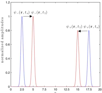
the same physical medium. Such problem is graphically shown in Figure 1, in which snapshots in timesto(in blue) andt1(in red) are taken for two arbitrary wavesψ+and
ψ−. In this Figure, the waveψ+ propagates in the−r
di-rection and the waveψ−propagates in+rdirection. One can say that waveψ− counterpropagates the waveψ+.
The interest in this problem resides in analyzing the resul-tant waveψin the physical medium. Counterpropagating
waves are present in many applied and theoretical investi-gations. Some applied researches involve the application of counterpropagating waves for manoeuvring, [4, 5] to manipulate objects in the microscale, [6] and in fiber op-tics for telecommunication. [7] Theoretical researches are associated with the breaking of symmetry in nonlinear resonators, [8] wave attraction in resonant systems, [9] and its dynamics in forced systems. [10]
Figure 1: Snapshots in two distinct times to and t1 of two
arbitrary wavesψ+ andψ−illustrating the contrapropagation
concept. Amplitudes are normalized by the amplitude of theψ+.
standing wave ratio (SWR) and the reflection coefficient acquire importance, which are associated with the ampli-tude of the individual waves. [14–16] However, aspects related to the propagation of the resultant wave – which are associated to the phase of the resultant wave – are not taken in to account.
Qualitatively, it is well-known that when the ampli-tudes of the counterpropagating waves are equal, the resultant wave presents a stationary pattern. It is merely an oscillation. It is a standing wave. But when the am-plitudes of the counterpropagating waves differ, the re-sultant wave still presents a travelling behavior. These situations are well explored in the books in the perspec-tive of the amplitude of the resultant wave. In the context of these systems, the SWR and the magnitude of the reflection coefficient respectively change from infinity to some finite value and from unity to some smaller value when the resultant pattern migrates from stationary to travelling. [14–16] Every literature in the field of wave phe-nomena stops the analysis of counterpropagating waves exactly at this point. No further discussions about the subject is presented. And from here the present work starts.
Waves are not just composed by amplitudes but also of phases. Opportunely, the existence of a phase is the unique restriction imposed by the wave equation [17] in its solution. To be a solution of the wave equation, a given arbitrary function f must depend of a phase φ, which relates the spatial coordinates r with the time t in an additive way. That is, in wave phenomena, as important as to analyze the wave amplitude is to analyze the phase of the wave. The existence of a phaseφthat is a combined function of the spatial coordinatesrand the timetis exactly what differs a wave from an oscillation.
In the same manner as mentioned above for the ampli-tude, the problem of counterpropagating waves can be explored qualitatively with a view on the phase of the resultant wave, by the means of its phase velocity. When the amplitudes of the individual waves are equal, the stationary situation, the phase velocity of the resultant wave is zero. However, when the amplitude of the individ-ual waves differ, the phase velocity of the resultant wave is not zero. That is, the phase velocity of the resultant wave has changed between both situations, to say from zero to some finite value. Moreover, since both situations are controlled by the individual amplitudes of the coun-terpropagating waves, so it is the phase velocity as well. In this way, some fundamental and conceptual questions arise in this subject: what is exactly the phase velocity of the resultant wave in this system? Does the phase velocity really depend of the amplitudes of the individual waves as the simple above observation qualitatively in-duces? If it depends, which is the expression for the phase velocity in this system? The absence of literatures that discuss this subject and answer the questions formulated right above motivates us to develop the present work.
In this way, the purpose of the present work is to ob-tain the resultant waveψ and to determine analytically
its phase velocity for a system composed by two counter-propagating waves. This paper is organized as follows. In section 2, the theory associated with the phase velocity is shortly discussed. In section 3, the resultant wave in the medium is analytically determined, being its phase velocity calculated. In section 4, the analytical results are confronted with numerical simulations. In section 5, the conclusions are presented. Finally, in section 6, the future works, which are consequences of all shown in this paper, are presented.
2. The theory
Textually, the phase velocity of a given wave is defined as the velocity an observer should develop for a given reference phase of the wave seems to be static, without any relative motion between the observer and the refer-ence point of the wave. Mathematically, defining a plane wave of amplitudeψo(r, t)and phaseφ(r, t)as [18,19]
ψ(r, t) =ψo(r, t)ejφ(r,t), (1)
and supposing a reference phase φo = φ(ro, to) to be followed, the phase velocity is such that in another spatial coordinater1 in timet1, the phase of the waveφremais constant
φ(ro, to) =φ(r1, t1) (2) which implies that
∆φ≡φ(r1, t1)−φ(ro, to) = 0. (3)
The rate of equation (3) within the interval of time∆tis ∆φ
For equation (4) to be valid in any instant of timet, the following limit has to be applied
lim
∆t→0
∆φ
∆t = 0, (5)
formally resulting in [18,19]
d
dtφ(r, t) = 0, (6) or
∂
∂tφ(r, t) +vf· ∂ ∂rφ(
r, t) = 0, (7)
in which ∂
∂rφ(r, t)is the gradient ofφ(r, t)andvf is the
velocity the observer must have to follow the reference phase of the wave, the phase velocity.
The right above equations (6) and (7) mathematically define which must be the phase velocityvf of the wave
ψ specified in equation (1). For evaluating the phase
velocity vf, it just must be knew the phase φ of the waveψof equation (1). This is what will be done in the
next section, in which the system of interest here, which is composed by two counterpropagating waves, will be specified and the resultant wave determined. With an analytical expression for the resultant waveψ, and
con-sequently for its phaseψ, it is possible then to determine
its phase velocity.
3. Analytical results
The present problem consists of two counterpropagating plane waves. The plane waves considered are also uni-form, which imply that its amplitudes, although might be different, are constants. One of the waves is repre-sented by ψ+ and the other by ψ−. Considering that both waves propagate in the same linear, homogeneous, and isotropic physical medium, so the resultant waveψ
in the medium is
ψ(r, t) =ψ+(r, t) +ψ
−(r, t). (8)
Assuming parallel polarization between waves, ψ+ =
ψ+eψ andψ−=ψ−eψ, the equation (8) becomes scalar
in the form
ψ(r, t) =ψ+(r, t) +ψ−(r, t). (9)
It is time to represent mathematically the individual wavesψ+ and ψ−. Consider that the waveψ+ is of the
form
ψ+(r, t) =ψo+ej(β·r+ωt) (10)
in which ψo+ is its constant plane wave amplitude, β
is its wave vector, and ω is its angular frequency. The counterpropagating problem is closed proposing another wave, to sayψ−, which propagates in opposite direction of the waveψ+ of equation (10). This waveψ− can be
mathematically represented in two distinct ways. One
consists of flipping the signal of the spatial term of the phaseφassociated with the wave ψ+ of equation (10)
ψ−(r, t) =ψo−ej(−β·r+ωt), (11)
and the other consists of flipping the signal of the tem-poral term of the phaseφassociated with the wave ψ+
of equation (10)
e
ψ−(r, t) =ψo−ej(β·r−ωt). (12)
In equations (11) and (12), ψo− is the constant ampli-tude of the plane waveψ−,βis its wave vector, andωis its angular frequency. As can be seen, the only difference that exists between the waveψ+ and both mathematical
representations of the waveψ−andψ−e , besides the direc-tions of propagation, resides on its constant amplitudes. In this way, the resultant waveψcan be represented as
ψ=ψo+ej(β·r+ωt)+ψo−ej(
−β·r+ωt), (13)
if the wave ψ+ of equation (10) and the wave ψ− of
equation (11) are inserted in equation (9), or the resultant waveψcan be represented as
e
ψ=ψo+ej(β·r+ωt)+ψo−ej(β
·r−ωt), (14)
if the wave ψ+ of equation (10) and the wave ψ− of
equation (12) are inserted in equation (9). Although physically equivalent, bothψandψerepresentations of the resultant wave are mathematically distinct. In this way, it can be also expected that the amplitudeψo and the phase φ are also different in both representations ψandψeof the resultant wave. And, as a consequence, distinct phase velocitiesvf will be potentially obtained in both representations.
In order to determine the phase velocity vf of the resultant wave, it is necessary to express the resultant wave, in both representations ψ andψ˜ right above, in the format of equation (1). When the representationψof the resultant wave of equation (13) is chosen, one finds that its phase velocity vf is described as a function of just the spatial coordinatesr. This approach is detailed in the next subsection 3.1 and called spatial approach, due to the functional dependence of the phase velocity of the resultant wave. However, when the representation
e
3.1. Spatial approach
For expressing the resultant wave ψ in the format of equation (1), one can rearrange the equation (13) as follows
ψ=ejωt·(ψ
o+ejβ·r+ψo−e−jβ·r). (15)
By the use of Euler and De Moivre relationejθ= cosθ+ jsinθ on the spatial terms e±jβ·r of the right above
equation, it is obtained
ψ = ej(ωt)·[(ψ
o++ψo−)cos(β·r)
+ j(ψo+−ψo−)sin(β·r)]. (16)
Looking for matching the equation (1) with the expres-sion right above of equation (16), it is obtained respec-tively the amplitudeψo
ψo(r) = p
(ψo++ψo−)
2cos2(β·r) + (ψ
o+−ψo−)
2sin2(β·r) (17)
and the phaseφ
φ(r, t) =ωt+ arctan ψ
o+−ψo− ψo++ψo−
tan(β·r)
, (18)
being the resultant waveψ of the form
ψ(r, t) =ψo(r)ejφ(r,t). (19)
Note that the resultant amplitude ψo is a function of the spatial coordinates r and the resultant phase φ is also a function of the time t. If ψo+ → ψo−, then ψo(r)→2ψo+cos(β·r),φ(r, t)→ωt, and consequently the resultant waveψis merely an oscillation, representing the well-known standing wave pattern. If|ψo+|>>|ψo−|, thenψo(t)→ψo+, andφ(r, t)→β·r+ωt, which is
es-sentially theψ+ wave, as should be predicted. Similarly,
if |ψo−| >> |ψo+|, then ψo(t) → ψo−, and φ(r, t) →
β·r−ωt, which is essentially theψ− wave, as should be also expected.
The phase velocity vf is directly obtained inserting equation (18) in equation (7) resulting in
vf = −ω β ·
ψ
o++ψo− ψo+−ψo−
cos2(β·r)
+ ψ
o+−ψo− ψo++ψo−
sin2(β·r)
eβ, (20)
in which eβ = β/β. One can directly verify that the phase velocityvf is a function of the spatial coordinates rwith mean value along one wavelengthλ= 2π/β
¯ vf=−ω
β ψ2
o++ψ2o− ψ2
o+−ψ2o−
eβ. (21)
It can be also observed that the phase velocity is indeed function of the individual wave amplitudesψo+andψo−, as the previous qualitative analysis in Section 1 - and that was the reason of this work - has predicted. If
ψo+→ψo−, thusvf →∞(and alsov¯f→∞), which is
the phase velocity of the standing wave if one considers the phase in equation (18), which in this caseφ(r, t)→ωt, beingβ= 0, as previously observed. If|ψo+|>>|ψo−|, thenvf → −ω
βeβ (and alsov¯f → − ω
βeβ), which is the phase velocity of theψ+ wave, as expected. Finally, if
|ψo−|>> |ψo+|, thenvf → ωβeβ (and alsov¯f → ωβeβ), which is the phase velocity of theψ− wave, as would be also expected.
The Figure 2 graphically illustrates the analytical re-sults for the resultant waveψ, the phaseφ, and the phase velocityvfobtained in this section. It has been considered
dimensionless amplitudesψo+ = 0.1 andψo− = 1, an-gular wave numberβ = 1rad/m, and angular frequency ω= 1rad/s. Panel (a) of Figure 2 illustrates the propa-gation of the resultant waveψ of equation (19). In this panel, the resultant waveψ is plotted along the spatial coordinatesrfor 3 distinct times,t= 0s, t= 0.1s, and t= 0.2s. Panel (b) of this same figure presents just the phase φof equation (18) along the spatial coordinates for these same times. Finally, the panel (c) of this figure shows the amplitude-dependance of the phase velocity vf of equation (20) along the spatial coordinates. In this
last panel, besides the previously mentioned value ofψo+,
it has been also consideredψo+ = 0.2, and ψo+ = 0.3.
One can observe in this last panel that the phase velocity always satisfies vf >0, since for each caseψo+ < ψo−, being the direction of propagation thus governed by the waveψ−.
A final analysis of the analytical results of this section must confront the behaviour of the phase velocity plotted in Figure 2(c) with the propagation of the resultant wave plotted in Figure Figure 2(a). For that, consider the spatial coordinates comprised in the interval1.5.r.3. Looking the phase velocity vf for ψo+ = 0.1, the blue
curve of Figure 2(c), one can observe that vf increases
with the increase of r. This behaviour of vf is in full
accordance with what is observed in Figure 2(a), in which, for a phase reference that turnsψ= 0, it can be observed, as time evolves, that the distance between the spatial coordinates in whichψ= 0also increases. In this way, since the interval of time between the snapshots of the resultant wave is constant, then the phase velocity of the resultant wave are also increasing in this interval.
The next subsection will treat of the second approach, which is associated with the representation ψe of the resultant wave described by equation (14).
3.2. Temporal approach
Instead of what has been performed in the previous section 3.1, evidencing the termej(β·r)in equation (14)
it is possible to obtain e
ψ=ej(β·r)·(ψ
o+ejωt+ψo−e
−jωt), (22)
which becomes e
ψ = ej(β·r)·[(ψ
o++ψo−)cos(ωt)
+ j(ψo+−ψo−)sin(ωt)], (23) when the Euler and De Moivre relation is applied to the temporal termse±jωtand some algebra is performed.
From the matching of equation (1) with the expres-sion between the squared brackets of equation (23), it is obtained respectively the amplitude ψeo
e ψo(t) =
q
(ψo++ψo−)2cos2(ωt) + (ψo+−ψo−)2sin2(ωt) (24) and the phase φ
e
φ(r, t) =β·r+ arctan ψ
o+−ψo− ψo++ψo−
tan(ωt)
, (25)
being the resultant wave ψeof the form
e
ψ(r, t) =ψeo(t)ejeφ(r,t). (26)
Note that the resultant amplitudeψeois a function of time t and the resultant phaseφeis also a function of space coordinatesr. Ifψo+→ψo−, thenψeo(t)→2ψo+cos(ωt),
e
φ(r, t) → β·r, and consequently the resultant wave e
ψ is merely an oscillation, representing the well-known standing wave pattern. If|ψo+|>>|ψo−|, thenψeo(t)→ ψo+, andφe(r, t)→β·r+ωt, which is essentially theψ+
wave, as should be predicted. Similarly, if|ψo−|>>|ψo+|,
then ψeo(t) → ψo−, and φe(r, t) → β·r−ωt, which is essentially the ψ− wave, as should be also expected.
The phase velocity vef is directly obtained inserting equation (25) in equation (7) resulting in
e vf=−ω
β ·
(ψo++ψo−)(ψo+−ψo−)
(ψo++ψo−)2cos2(ωt) + (ψo+−ψo−)2sin2(ωt)
eβ. (27)
One can directly verify that the phase velocity evf is a function of the timetwith mean value along one period T = 2π/ω
hvefi=−ω
βsign(ψo+−ψo−)eβ, (28) in whichsign(x) = 1forx >0,sign(x) =−1forx <0, andsign(x) = 0 forx= 0.
In the same manner as performed in the previous sub-section, it can be also observed that the phase velocity is indeed function of the individual wave amplitudes ψo+andψo−, as the previous simple qualitative analysis in Section 1 and that was the reason of this work -has predicted. If ψo+ → ψo−, thus evf → 0 (and also
hevfi → 0), which is the phase velocity of the stand-ing wave. If |ψo+| >> |ψo−|, then evf → −ωβeβ (and also hvefi =−ω
βeβ), which is the phase velocity of the ψ+ wave, as expected. Finally, if|ψo−|>>|ψo+|, then
e vf → ω
βeβ (and also hvefi = ωβeβ), which is the phase
velocity of theψ− wave, as would be also expected. In this way, the phase velocityevf of the resultant wave can be adequately adjusted to absolute values smaller than the phase velocityω/βof the individual plane waves.
As performed in the previous section, the Figure 3 graphically illustrates the analytical results for the re-sultant wave ψe, the phase φe, and the phase velocity e
vf obtained in this section. It has been also considered
dimensionless amplitudesψo+ = 0.1 andψo− = 1, an-gular wave numberβ= 1rad/m, and angular frequency ω= 1rad/s. Panel (a) of Figure 3 illustrates the propa-gation of the resultant waveψeof equation (26). In this panel, the resultant wave ψeis plotted along the timet for 3 distinct spatial coordinates,r= 0m,r= 0.1m, and r= 0.2m. Panel (b) of this same figure presents just the phaseφeof equation (25) along the time for these same
spatial coordinates. Finally, the panel (c) of this figure shows the amplitude-dependance of the phase velocity e
vf of equation (27) along the time. In this last panel,
be-sides the previously mentioned value ofψo+, it has been
also consideredψo+= 0.2, and ψo+= 0.3. One can also
observe in this last panel that the phase velocity always satisfiesevf >0, since for each of these casesψo+< ψo−, being the direction of propagation thus governed by the waveψ−.
Similarly with what has been done in the previous section, to conclude the analysis of the analytical results of this section, one must confront the behaviour of the phase velocity plotted in Figure 3(c) with the propaga-tion of the resultant wave plotted in Figure 3(a). For that, consider the interval of time1.5.t.3. Looking the phase velocityvef for ψo+ = 0.1, the blue curve of
Figure 3(c), one can observe thatevf decreases with the
increase oft. Again, this behaviour ofevf in this interval
of time is in full accordance with what can be seen in Figure 3(a), since the time elapsed between each cross-ing ofψeby0increases. In this way, since the distance between the spatial coordinates in which the resultant wave is analysed is constant, then the phase velocity of the resultant wave are also decreasing in this interval.
3.3. The equivalence between both approaches
The spatial and temporal approaches presented before produced different expressions for the phase and ampli-tude of the resultant wave. However, it is expected that the analytical results for the wave ψ of equation (19) andψeof equation (26), which involves the product of the resultant wave amplitudes and phases in both repre-sentations, describes absolutely the same wave, although they have different mathematical representations. Rigor-ously, the numerical results shown in the next section 4 comprove that the analytical equations (19) and (26) for the resultant wave in both representations are physically equivalent and are absolutely correct. However, quanti-ties derived of just the amplitude or of just the phase (not of the product of both) of the resultant wave do not necessary match for every spatial coordinate r or the timet. This is the case of the phase velocity of the resultant wave, which is an expression derived from just the phase of the resultant wave. It is then necessary a detailed inspection of these expressions to connect the results produced by both approaches.
For evaluating compatibility between the phase ve-locities vf andevf it is necessary that the reference in the wavesψandψeadopted is the same. If the reference adopted is exactly the same in both representations, it is expected the expressions of the phase velocity in both approaches produce the same result. An adequate phase reference to choose is
φ(r, t) =φe(r, t) =mπ/2, (29)
sinceRe{ψ}= Re{ψe}= 0, eliminating the influences of
the different aspects of the resultant wave amplitude in both representations. m= 2n+ 1, and nis an integer number. Inserting this reference phase in equation (18) results in
tan(mπ/2−ωt) =
ψo+−ψo− ψo++ψo−
tan(β·r), (30)
while inserting in equation (25) results in
tan(mπ/2−β·r) =
ψo+−ψo− ψo++ψo−
tan(ωt). (31)
Considering thattan(mπ/2−x) = 1/tan(x), then both equations (30) and (31) produces exactly the same ex-pression
ψo+−ψo− ψo++ψo−
tan(ωt) tan(β·r) = 1. (32)
Essentially, the equation (32) establishes, for any given timetin whichφ=mπ/2, which is the spatial coordinate rin which theφeis alsomπ/2. That is, this is the relation between the spatial coordinatesrand the timetto follow the same reference phase in both spatial and temporal approaches employed to represent the resultant wave. In this situation, since the reference phase adopted is the same in the approaches, it is expected that the phase velocities vf andvef match its results.
The figure 4 shows the absolute value of the phase velocity vf along the spatial coordinatesr=rer. Also,
in this figure, the phase velocity evf is presented. The
phase velocityevfis outlined along the spatial coordinates
r by the means of the equation (32). For each spatial coordinatevf is plotted, the corresponding value of the
timet is obtained through the equation (32) and then e
vf is plotted. This procedure assure that any value of
vf is compared with evf for exactly the same reference
phase. It can be observed a perfect agreement between both expressions of the phase velocity. For completeness, the figure 5 presents the results for the phase velocity e
vf along the timet together with the phase velocityvf.
The phase velocityvf is determined calculating, for each
time t, which is the corresponding spatial position r through the equation (32). It can be observed again a nice agreement. In figure 4 and 5, it is adoptedψo+= 0.1
andψo−= 1, which are dimensionless, with ω= 1rad/s andβ = 1rad/m.
The analytical expressions of both approaches satisfied the expected results in the limit situations explored above in each subsection. Also, it has been observed that both approaches are equivalent when the same reference phase of the resultant wave is considered. However, for full vali-dation, the analytical expressions obtained for the phase velocity through both approaches must be confronted with the results obtained from the direct numerical sim-ulation of equation (9) with equation (10) and equation (11) or equation (12). In this way, in the next section, a direct comparison between the analytical and numerical results for the resultant wave and its phase velocity will occur.
4. Comparison with numerical
simulations
The analytical results presented in the previous section 3 are confronted here with numerical simulations of the counterpropagating waves. In Figure 6 and Figure 7, as the first comparison, it is shown the analytical and nu-merical results for the resultant waveψrespectively as a function of timetand of spatial coordinatesr=rer. The numerical results consist of the direct simulation of the real part of the resultant waveψdescribed in equation (9)
with the individual waves of equation (10) and equations
Figure 5:Comparison between the phase velocitiesvf, plotted with crosses, andevf, plotted as a continuous line, for the same reference phase along the timet.
Figure 6: Comparison between the numerical and analytical results for the resultant wave ψ in the medium as a function of timetforr= 4m. The results of the spatial and temporal
approaches are respectively represented with crosses and circles.
Figure 7: Comparison between the numerical and analytical results for the resultant wave in the medium as a function of spatial coordinater fort= 1s. The results of the spatial and
temporal approaches are respectively represented with crosses and circles.
(11) or (12), depending of the representation adopted. The analytical results consist in evaluating the real part of the resultant wave of equation (19) with the resultant amplitude of equation (17) and the resultant phase of equation (18), for the spatial approach (represented with crosses), and in to evaluate the real part of the resultant wave of equation (26) with the resultant amplitude of equation (24) and the resultant phase of equation (25), in the case of the temporal approach (represented with circles). A perfect agreement with numerical simulations is achieved in both analytical approaches as expected. The dimensionless waves amplitudes are ψo+= 0.2and
ψo−= 1, the angular wave number isβ = 1rad/m, and the angular frequency isω= 1rad/s. Perfect agreement is also found for other values of waves amplitudes, wave number, and angular frequency, being satisfactory to com-prove that the analytical expressions for the resultant waveψin both approaches are correct.
successive spatial coordinates r as time t evolves. For each displacement∆r, it is possible then to calculate the necessary time interval∆t. Independently of following the spatial or temporal coordinates, the absolute value of the phase velocity estimated numerically is
vfn≈∆r/∆t, (33)
in which the subscriptnstands for numeric. To follow spatial or temporal coordinates will be suitable when the comparison of the numerical results for the phase velocity occurs respectively with the analytical results provided by the spatial and temporal approaches. Since the resultant waveψ is periodic, it only must be assured that∆r <<2π/β and∆t <<2π/ω, avoiding ambiguity problems when tracking the reference phase φn of the wave respectively along the spatial coordinatesror the timet. This numeric procedure will be applied right below when the analytical results from both approaches will be confronted with the numerical results for the phase velocity.
Figure 8 and Figure 9 presents the results along the spatial coordinates r for respectively ψo+ = 0.1 and
ψo+= 0.2in distinct times. This is the only difference
between both Figures. For both,ψo−= 1,β= 1rad/m, andω= 1rad/s. For simplicity, the reference phaseφn chosen is such that turns the resultant waveψ= 0. This assumption substantially simplifies the tracking of the reference phaseφn along the spatial coordinatesr, once the amplitude of the resultant wave also depends of the spatial coordinates r, and it can induces to errors in following the reference phase pointφn. Theψ= 0curve is plotted together in the panels (a) of Figures 8 and 9
Figure 8:Cumulative plots of the resultant waveψalong the spatial coordinaterfor 100 successive timestnwith∆tn= 0.01s
are shown in panel (a). A comparison between the numerical and analytical results for the absolute value of the phase velocity vf is shown in panel (b). In both panels,ψo+= 0.1.
Figure 9:Cumulative plots of the resultant waveψ along the spatial coordinaterfor 100 successive timestnwith∆tn= 0.01s
are shown in panel (a). A comparison between the numerical and analytical results for the absolute value of the phase velocity vf is shown in panel (b). In both panels,ψo+= 0.2.
for analysis purposes. The reference phaseφn is tracked along1s≤tn≤2s, in steps of∆tn= 0.01s. The resultant wave ψ along the spatial coordinatesr for each one of these timestnis cumulatively plotted in the panels (a) of Figures 8 and 9. In these Figures, each color represents the resultant wave picture along the spatial coordinates rin each one of the timestn. The total number of curves plotted in the panels (a) of Figures 8 and 9 are 100, which shows to be adequate to describe the phase velocity in the interval of spatial coordinates1.5m≤r≤4mwith a reasonable accuracy. The crossing by ψ = 0 of the ψ(r, tn)for each timetn occurs in a spatial coordinatern and is detached by a ’+’ sign. The spatial displacement ∆rof equation (33) computed numerically is exactly the spatial displacement∆rn between each consecutive ’+’ sign. Figure 10 details and illustrates how∆ris evaluated numerically for the first two waves plotted in Figure 8. Figure 10 represents a zoom of Figure 8 for −0.01 ≤ ψ ≤ 0.05 and 1.5m ≤ r ≤ 4m. The interval of time
∆t of equation (33) is exactly the previously specified ∆tn= 0.01s, a constant. The phase velocity is numerically calculated inserting all the spatial displacement ∆rn computed with∆tn = 0.01sin equation (33). Panel (b) of Figures 8 and 9 compares the numeric and analytical results for the absolute value of the phase velocity vf
for respectively the wave amplitudes ψo+ = 0.1 and
ψo+ = 0.2 described above. The analytical result for
the phase velocity vf uses the expression described in
equation (20). Nice agreement can be observed.
Similarly, the Figure 11 and Figure 12 presents the results for respectivelyψo+= 0.1andψo+= 0.2along
Figure 10: A detailed description of the crossing spatial coordi-nates byψ= 0of the first two waves plotted in Figure 8. The
difference between this consecutive crossing spatial coordinates is exactly the displacement interval ∆r used to evaluate the phase velocity in this specific interval.
Figure 11: Cumulative plots of the resultant waveψealong the timetfor 100 successive spatial positionsrnwith∆rn= 0.01m
are shown in panel (a). A comparison between the numerical and analytical results for the absolute value of the phase velocity e
vf is shown in panel (b). In both panels,ψo+= 0.1.
difference between both Figures. For both,ψo− = 1,β = 1rad/m, and ω = 1rad/s. For simplicity, the reference phaseφnchosen is such that turns the resultant waveψ= 0. This assumption substantially simplifies the tracking of the reference phase φn along the time t, once the amplitude of the resultant wave also depends of the timetin this approach, and it can induces to errors in following the reference phase pointφn. Theψ= 0curve
Figure 12:Cumulative plots of the resultant waveψealong the timetfor 100 successive spatial positionsrnwith∆rn= 0.01m
are shown in panel (a). A comparison between the numerical and analytical results for the absolute value of the phase velocity e
vf is shown in panel (b). In both panels,ψo+= 0.2.
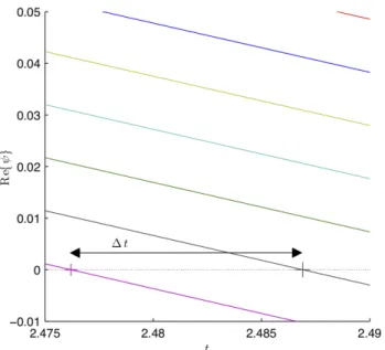
is plotted together in the panels (a) of Figures 11 and 12 for analysis purposes. The reference phaseφn is tracked along 1m ≤ rn ≤ 2m, in steps of ∆rn = 0.01m. The resultant waveψalong timetfor each one of these spatial coordinatesrnis cumulatively plotted in the panels (a) of Figures 11 and 12. In these Figures, each color represents the resultant wave picture along time t in each one of the spatial coordinatesrn. The total number of curves plotted in the panels (a) of Figures 11 and 12 are 100, which shows to be adequate to describe the phase velocity in the interval of time2.5s≤t≤3.5swith a reasonable accuracy. The crossing byψ= 0of theψ(rn, t)for each spatial coordinaternoccurs in a timetn and is detached by a ’+’ sign. The interval of time∆t of equation (33) computed numerically is exactly the interval of time∆tn between each consecutive ’+’ sign. Figure 13 details and illustrates how∆tis evaluated numerically for the first two waves plotted in Figure 11. Figure 13 represents a zoom of Figure 11 for−0.01≤ψ≤0.05and2.475s≤t≤
2.49s. The spatial displacement∆rof equation (33) is exactly the previously specified∆rn = 0.01m, a constant. The phase velocity is numerically calculated inserting all the∆tn computed with∆rn= 0.01min equation (33). Panel (b) of Figures 11 and 12 compares the numeric and analytical results for the absolute value of the phase velocityvffor respectively the wave amplitudesψo+= 0.1
and ψo+ = 0.2described above. The analytical result
for the phase velocityvf uses the expression described in
Figure 13:A detailed description of the crossing times byψe= 0
of the first two waves plotted in Figure 11. The difference between this consecutive crossing times is exactly the time interval∆t
used to evaluate the phase velocity in this specific interval.
5. Conclusions
The superposition of plane waves in a physical medium can produce a resultant wave with a phase velocity dis-tinct from the former plane wave components. Such is the case of a wave incident obliquely over an infinite and perfect conducting surface, in which the phase velocity of the resultant wave in the incident medium becomes also – although it remais constant – a function of the incidence angle.
In the present situation of counterpropagating waves, it was demonstrated that the superposition of plane waves can also produce a resultant wave with phase velocity that depends of the spatial coordinate r or the time t, depending of the approach adopted. As shown, both approaches are equivalent, since they provide results that are identical to each other when the same reference phase is considered.
Considering the temporal approach, mathematically, the phase velocity of the resultant wave could be ex-pressed asevf =vplanef ·f(ψo+, ψo−, t), in whichvplanef =
ω/βrepresents the absolute value of the well-known phase velocity expression for the plane waves, such asψ+ and
e
ψ−are in this work. The dimensionless factorf accounts the propagative effects – resultant of the superposition of counterpropagating waves – in the present case, which is a function of the amplitudes of the individual waves, ψ+ andψ−, and the time t. It must be also observed
that, althoughvef is function of timet,hevfiis a constant
exactly equal in magnitude tovfplane. This is physically reasonable, since in this case there is no changes in the physical medium or boundaries, which are generally the mechanisms responsible to effectively impact the phase
velocity. Over a period2π/ω, the resultant waveψ prop-agates in the same way as the individual wavesψ+and
e
ψ− alone in the physical medium.
One interesting feature identified in this work is asso-ciated with the fact of the phase velocity of the resultant wave to depend of the individual wave amplitudes. This interesting feature can be explored in electromagnetics as will be right now discussed. In charged particle accelera-tors, resonant interaction between charged particles and the generated electromagnetic waves is intended to cause particle acceleration. If the resultant wave of the system studied in this work is electromagnetic and propagates in a plasma, the resonant interaction of the resultant wave with the charged particles of the medium can be controlled by the amplitudes of the individual waves. More, by counterpropagation, superluminal waves can lower down its phase velocities to interact resonantly with charged particles of the medium.
This mechanism identified in this work is relevant to develop new charged particle acceleration concepts and structures. The controlling feature of the phase velocity of the resultant wave through the individual amplitudes of the plane wave components is practical from the imple-mentation point of view. Although the amplitude control can occur through two distinct generators, it is more suitable to establish counterpropagation through reflec-tion. In this way, instead of controlling individually the amplitude of the counterpropagating waves, one can just control the reflection coefficient, and then so the phase velocity of the resultant wave for accelerating purposes. By the end, the analytical expressions in both rep-resentations predict the well-know results of the limit situations involving the amplitudes of the individual waves. Perfect agreement of both representations with the numerical simulations is also found.
6. Future works
Future works will explore this amplitude-dependant char-acteristic of the phase velocity of the resultant wave in the wave-particle interaction phenomena in a electro-magnetic system. For that, counterpropagating waves will be considered to evolve in a plasma, and the res-onant interaction between the resultant wave and the charged particles of the medium will be analysed. An analytical description of how the individual counterprop-agating wave amplitudes control the resonant interaction is expected to be obtained.
References
[1] J.M. Serra, M.C. Brito, J.M. Alves and A.M. Vallera, Eur. J. Phys.25, 5 (2004).
[2] A.C.F. Santos, W.S. Santos and C.E. Aguiar, Eur. J. Phys.34, 3 (2013).
[4] S. Sefati, I. Neveln, M.A. MacIver, E.S. Fortune and N.J. Cowan, inProceedings of the 4th IEEE RAS/EMBS International Conference on Biomedical Robotics and Biomechatronics, (IEEE RAS/EMBS, Rome, 2012), p. 1620.
[5] O.M. Curet, N.A. Patankar, G.V. Lauder and M.A. MacIver, J. R. Soc. Interface8, 1041 (2011).
[6] A. Grinenko, C.K. Ong, C.R.P. Courtney, P.D. Wilcox and B.W. Drinkwater, Appl. Phys. Lett. 101, 233501 (2012).
[7] S. Pitois, J. Fatome and G. Millot, Opt. Express 16, 6646 (2008).
[8] L. Bino, J.M. Silver, S.L. Stebbings and P. Del’Haye, Scientific Reports7, 43142 (2017).
[9] M. Grenier, H.R. Jauslin, C. Klein and V.B. Matveev, Journal of Mathematical Physics52, 082704 (2011). [10] C. Martel, E. Knobloch and M. Vega, Physica D:
Non-linear Phenomena137, 94 (2000).
[11] C.A. Balanis, Advanced Engineering Electromagnetics (John Wiley & Sons, New York, 1989), 1st ed.
[12] R.E. Gibbs, The Physics Teacher36, 2 (1998). [13] J.M. Blair, Am. J. Phys.50, 8 (1982).
[14] D.K. Cheng,Field and Wave Electromagnetics (Addison-Wesley, New York, 1989), 2nd ed.
[15] S. Ramo, J.R. Whinnery and T. van Duzer,Fields and Waves in Communication Electronics (John Wiley & Sons, New York, 1993), 3rd ed.
[16] C.T.A. Johnk,Engineering Electromagnetic Fields and Waves(John Wiley & Sons, New York, 1988).
[17] C.K.C. Lieou, Eur. J. Phys.28, 4 (2007).
[18] J.D. Jackson,Classical Electrodynamics(John Wiley & Sons, New York, 1998), 3rd ed.