A REVIEW OF SWEPT AND BLENDED WING BODY PERFORMANCE UTILIZING EXPERIMENTAL, FE AND AERODYNAMIC TECHNIQUES

371

A REVIEW OF SWEPT AND BLENDED WING BODY PERFORMANCE

UTILIZING EXPERIMENTAL, FE AND AERODYNAMIC TECHNIQUES

1_{Hassan Muneel Syed,} 2_{M. Saqib Hameed &} 3_{Irfan A. Manarvi}

1_{Department of Aeronautics and Astronautics, Institute of Space Technology, Islamabad, Pakistan} 2,3_{Department of Mechanical Engineering, HITEC University, Taxila Education City, Pakistan}

Email: [email protected], [email protected], [email protected]

ABSTRACT

In this paper an effort is made for prediction of aerodynamic behavior of a BWB using design tools such as IFL, PrADO. A set of wings was constructed by parametric variation on wing sweep. The CL, CD and Cm were investigated in steady state CFD of BWB at Mach 0.3 and through wind tunnel experiments on 1/6th model of BWB at mach 0.1. From CFD analysis pressure variation, Mach number contours and turbulence area was observed. Wing/fuselage thermal model was also investigated for stresses on wings and fuselage using nodal temperature derivation method at wing/fuselage interface. Elastic behavior of high-lift geometrically complex wing along with multiple components (flap, slat, weapons, pods etc) was studied. Also swept wing of a fighter aircraft was investigated using ANSYS and regions of high deflection, stress and strain were located.

Keywords: CL = Coefficient of Lift, CD = Coefficient of Drag, CFD = Computational Fluid Dynamics, BWB =

Blended Wing Body, UAV = Unmanned Aerial Vehicle, CDo = Coefficient of drag at zero lift, Po= total

pressure (Pa), α = angle of attack (degree)

1. INTRODUCTION

372

and implementation of advanced modeling and analysis capabilities of a large toolbox ―Preliminary Aircraft Design and Optimization Program‖ (PrADO) were used for both structure and aerodynamics of BWB [10]. This effort presents a comparison of swept wing with blended wing bodies using the techniques of structural and aerodynamic analyses.

2.APPLICATION OF FE TECHNIQUES ON A SWEPT WING OF A FIGHTER AIRCRAFT

Technique of FEM was used to establish the stress concentration on the wing. The following steps were taken in typical FE software (ANSYS version 9.0).

2.1 Modeling of swept wing geometry

Swept wing was modeled in ANSYS using NACA 66-012 airfoil. First step of modeling was insertion of key points following the coordinates of NACA 66-012 airfoil at different sections of wing. Then, areas were created using these airfoils and therefore a single solid wing was modeled by adding up these areas. The solid model of swept wing is shown in Fig. 1.

2.2 Element type selection:

Solid45 was chosen to mesh the solid volume. Element with plasticity, creep, swelling, stress stiffening, large deflection, and large strain capabilities shown in Fig.2 was refined for discontinuities.

2.3 Material properties:

Material was assigned with properties, modulus of elasticity as 56.8GPa and Poisson’s ratio as 0.33.

Fig. 1 Solid Model of swept wing in ANSYS Fig. 2 Element type used; Solid45(Ansys)

2.4 Mesh size control:

Lines of airfoils were divided into 30 parts whereas; lines along extrusion were divided into 60 parts, as shown in Fig. 3. Then, the volume was meshed using this size control, as shown in Fig. 4.

Fig. 3 Solid Model mesh size control Fig. 4 3-D Mesh over the swept wing

2.5 Application of loads:

373

Fig. 5 Application of displacement loads at root and pressure loads at bottom surface of wing

2.6 Solution of load set:

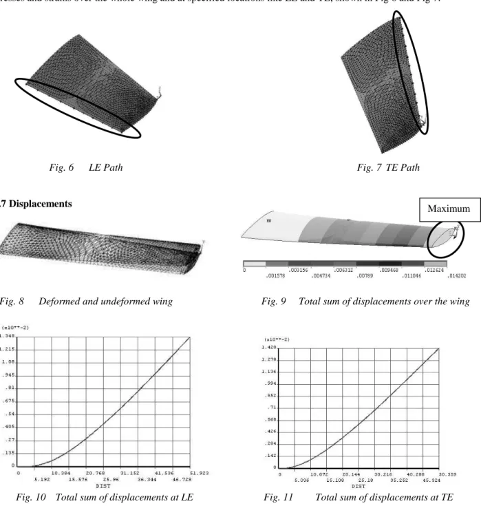
At this stage FE model was solved and all the system matrices were solved collecting the values of deflections, stresses and strains over the whole wing and at specified locations like LE and TE, shown in Fig 6 and Fig 7.

Fig. 6 LE Path Fig. 7 TE Path

2.7 Displacements

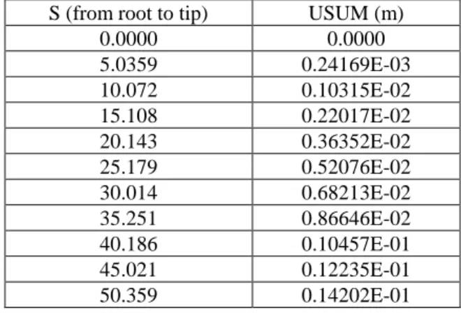
Fig. 8 Deformed and undeformed wing Fig. 9 Total sum of displacements over the wing

Fig. 10 Total sum of displacements at LE Fig. 11 Total sum of displacements at TE

374

Table 1: Total Displacements at LE Table 2: Total Displacements at TE

2.8 Von Misses Stresses

Fig. 12 Von misses stresses Fig. 13 Total stresses at LE

Table 3: T o t a l s t r e s s e s at LE

Fig.

14 Total stresses at TE

3. AERODYNAMIC AND STRUCTURAL TECHNIQUES APPLIED ON SWEPT WINGS

3.1 Thermal analysis of wing/fuselage interface

The thermal gradients over the wing and other fuselage structures are identified.

S (from root to tip) USUM (m)

0.0000 0.0000

5.2961 0.84455E-04

10.281 0.60004E-03

15.265 0.15315E-02

20.146 0.27502E-02

25.235 0.42283E-02

30.115 0.57468E-02

35.048 0.74022E-02

40.240 0.92346E-02

45.173 0.11020E-01

51.923 0.13484E-01

S (from root to tip) USUM (m)

0.0000 0.0000

5.0359 0.24169E-03

10.072 0.10315E-02

15.108 0.22017E-02

20.143 0.36352E-02

25.179 0.52076E-02

30.014 0.68213E-02

35.251 0.86646E-02

40.186 0.10457E-01

45.021 0.12235E-01

50.359 0.14202E-01

S (from root to tip) SEQV (Mpa)

0.0000 0.46349

5.2961 0.68140

10.281 0.64827

15.265 0.41738

20.146 0.52273

25.235 0.35755

30.115 0.22137

35.048 0.13512

40.240 0.10082

45.173 0.074018

51.923 0.012063

375

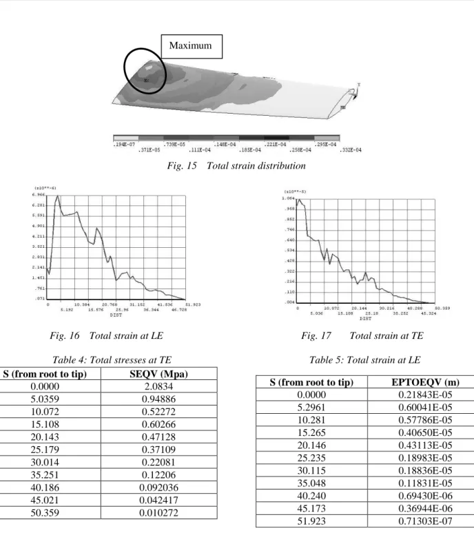
Fig. 15 Total strain distribution

Fig. 16 Total strain at LE Fig. 17 Total strain at TE

Table 4: Total stresses at TE Table 5: Total strain at LE

The situations that intensify thermal gradient because of thermal shift in environmental interactions are evaluated by a series of possible flight paths.

3.2 Creating of geometry and generation of mesh

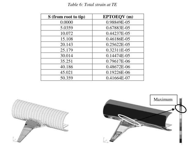
A thermal FE model of fuselage/wing is created for 728 Jet, Fig 18.

3.3 Method used for thermal analysis

MSC. Patran thermal is used for thermal calculations and QTRAN is used for further solutions. This is technique is based on thermal network where thermal resistances potentials (capacitors) are collectively used. Resistor-capacitor data is developed through translation of elements from FE element data through a routine in the PATQ code. For solution, QTRAN code used a predictor-corrector algorithm.

S (from root to tip) EPTOEQV (m)

0.0000 0.21843E-05

5.2961 0.60041E-05

10.281 0.57786E-05

15.265 0.40650E-05

20.146 0.43113E-05

25.235 0.18983E-05

30.115 0.18836E-05

35.048 0.11831E-05

40.240 0.69430E-06

45.173 0.36944E-06

51.923 0.71303E-07

S (from root to tip) SEQV (Mpa)

0.0000 2.0834

5.0359 0.94886

10.072 0.52272

15.108 0.60266

20.143 0.47128

25.179 0.37109

30.014 0.22081

35.251 0.12206

40.186 0.092036

45.021 0.042417

50.359 0.010272

376

Table 6: Total strain at TE

Fig. 18 FE model of wing/fuselage interface [2] Fig. 19 Temperature contours at high altitudes (Top) [2]

3.4 Material/element properties and boundary conditions

Temperature dependent material properties of steel, aluminum, fuel and air are added to the definition of model. Boundary conditions include boundary temperatures, convection, radiation and fuel modeling. For convection boundary conditions, defining temperature is necessary. Based on aircraft speed and altitude, the boundary layer, or adiabatic wall temperature is calculated. Values are convincing from empirical correlations of flow conditions for heat transfer coefficients. Over the all exposed regions of the wing and fuselage, an average film coefficient is used. For the components at various altitudes in normal flight mission, steady state estimations are made. Flux term is 1-2% of convection term, so additional modeling is not required. To handle the changing fuel level in the tanks, a methodology is created. A boundary condition consists of two components is made up, first component is connected to fuel ―fluid node‖ and second with air ―fuel node‖. 0% and 100% connections are set to fuel and air respectively as the falls below. Variation in connections with percent of fuel and air comes during the transition phase. Temperature contours obtained from model are shown in Fig 19 and Fig 20.

3.5 Implementation of Euler equations on swept wings:

The basis of the design method is a computer program FLO87. It uses a cell-centered finite volume scheme to solve three dimensional Euler equations. Several swept wings are optimized to test the method. Restriction on minimum thickness is applied, wing planform is fixed and sections are free to be changed by the design method.

The initial wing is taken with unit span and leading edge sweep of 30 degree. The pressure distribution is shown in Fig 21. At Mach number 0.85, the results of the calculations with the lift coefficient forcefully attain the value of 0.5 are shown in Fig 22 and Fig 23. Plots are shown the initial wing geometry and pressure distribution, with modification that are made in wing geometry and pressure distribution after 40 design cycles. The inviscid drag value is reduced from 0.0207 to 0.0113.

S (from root to tip) EPTOEQV (m)

0.0000 0.98849E-05

5.0359 0.67883E-05

10.072 0.44237E-05

15.108 0.46186E-05

20.143 0.25622E-05

25.179 0.32311E-05

30.014 0.14474E-05

35.251 0.79617E-06

40.186 0.48672E-06

45.021 0.19226E-06

50.359 0.41664E-07

377

Fig. 20 Temp. contours (high altitudes) Bottom[2] Fig. 21 Original wing section& required pressure distribution[7]

Fig. 22 Drag reduction at M = 0.85, Fixed lift mode [7] Fig. 23 Upper surface pressure [7]

The final geometry is analyzed with another method using computer program FLO67 to verify the solution. When the program is run and full convergence is achieved, it is found that, at Mach number 0.85, better estimate of the drag coefficient of the redesigned wing is 0.0094 and with lift coefficient of 0.5, lift to drag ratio is 53. Fig 24 shows the results of this case.

3.6 Aeroelastic analysis of high lift swept wings:

ASTM 579 steel is used to make the high lift wind tunnel model to withstand the high pressure loadings. In terms of IGES patches, structural model is extracted from CAD geometry definition of wind tunnel model. High lift wing CFD geometry is shown in Fig 25.

For final structural model, Fig 26, the flap tracks and slat tracks are modeled on the basis that, same degree of freedom on structural nodes of main wing and slat/flap. Beam elements are used to model the slats. Static aeroelastic analysis of high lift wing was carried out, at an angle of attack α = 12 degree, Mach number M = 0.2 and free stream dynamic pressure q = 6.5 kPa.

In two steps of an iterative algorithm used to carry out aerostatic simulation, surface pressure, surface force and corresponding deformations are obtained. The final deformed high-lift wing is shown in Fig 28, computed deformations on structural grid is shown at left and computed deformed aerodynamic grid of the high-lift wind tunnel model is shown at right. As a function of wing span for deformed and rigid wings, the heights (smallest) between the flap & main wing and slat & main wing are shown in Fig 29 & Fig 30.

i. To obtain surface pressure, flow analysis is carried out using unstructured flow solver, and unstructured surface grid is shown in Fig 27.

Wing initially at α = -1.340o Cl = 0.5001 Cd = 0.0207

Design iterations at α = -0.235o Cl = 0.5000 Cd = 0.0113

Wing initially at α = -1.340o

Cl = 0.5001 Cd = 0.0207

Design iterations at α = -0.235o

Cl = 0.5000 Cd = 0.0113

378

ii. Surface force distribution and corresponding surface deformation is obtained through structural analysis.

Fig. 24 Redesigned wing (FLO67 check) M = 0.85, α = -0.240o Cl = 0.4977, Cd = 0.0094 [7]

Fig. 25 CFD model of high lift wing [9] Fig. 26 Structural model developed for high lift wing [9]

Fig. 27 Unstructured computational surface grid [9] Fig. 28 Final deformed high-lift wing [9] (Contour line with same deflection in vertical (z-direction) can be seen)

3.7 Pressure distribution over swept wing

At selected section, static pressure distributions are shown at Fig. 31 for a high-lift swept wing at Mach number 0.82 and angle of attack equals to 2o.

-ve

+ve

-ve

+ve

+ve -ve

Span station z = 0 Span station z = 0.312

Span station z = 0.625 Span station z = 0.937

-ve

+ve

379

Fig. 29 Height of the flap-gap [11] Fig. 30 Height of the slat-gap [11]

Fig. 31 Distribution of static pressure over a high-lift wing [11]

Table 7: Pure aerodynamic performance [8]

4.AERODYNAMIC AND EXPERIMENTAL TECHNIQUES APPLIED ON BLENDED WING BODY

4.1 Geometric, aerodynamic and FE models of BWB using PrADO:

Multiple trapezoidal patches defined by twist, dihedral, root and tip chord, leading edge sweep and wing sections are used to make lifting surfaces. Upper and lower skin, spars with web and girder are constitutes of load carrying structure of lifting surfaces. Non structural mass elements are used to model leading and trailing edge components. Characteristic cross-sections along the longitudinal axis are used to define the geometry of fuselage. Fig 32 shows the geometric model of BWB.

Mach Sweep CL CD CD.tot ML/D √ML/D

0.85 35◦ 0.500 153.7 293.7 14.47 15.70 0.84 30◦ 0.510 151.2 291.2 14.71 16.05 0.83 25◦ 0.515 151.2 291.2 14.68 16.11 0.82 20◦ 0.520 151.7 291.7 14.62 16.14 0.81 15◦ 0.525 152.4 292.4 14.54 16.16 0.80 10◦ 0.530 152.2 292.2 14.51 16.22

0.79 5◦ 0.535 152.5 292.5 14.45 16.26

Rigid

380

Fig. 32 Example of geometric model of BWB configuration [10]

Above described geometric configuration is further used to develop models for structural and aerodynamic analyses. Finite element and aerodynamic models are provided by a multi-model generator, Fig 33 & Fig 34 respectively. The symmetry plane of FE model is created by single point constraints and configuration is restricted to half of the model. Symmetry is assumed and considered in analysis for aerodynamic analyses.

Fig. 33 Example of FE model for analyses [10] Fig. 34 Example of aerodynamic model for analyses [10]

4.2 Implementation of CFD approach:

Stage1: Fig 35 shows 3 views of BWB planned during its preliminary design. 3D drawing is extracted in CATIA using its mathematical model obtained from derivation of geometric equations.

Stage2: 3D model developed in CATIA is converted into CFD meshed element in GAMBIT. Then the suitable meshed model is imported to FLUENT for its subsonic flow analysis at Mach number from 0.1 to 0.3 corresponding to Reynolds’s number 4.66 x 106

& 1.4 x 107 respectively.

FE model consists of body, wing, and winglet. Membrane, beam and rod elements are used. Single point constraint is used in symmetry plane. Aerodynamic, inertial, and internal pressure loads are applied.

381

Fig. 35 3-views of BWB used for analysis [1] 4.3 Results obtained from CFD:

Fig. 36 Contours of pressure coefficient at upper surface Fig. 37 Contours of pressure coefficient at upper Surface At α = 0o

M = 0.3 [1] At α = 35o M = 0.3 [1]

Fig. 38 Contours of Mach number at upper surface Fig. 39 Contours of Mach number at upper surface

At α = 0o _{M = 0.3[1] At α = 35}o _{M = 0.3 [1]}

4.4 Implementation of wind tunnel testing and obtained results

UiTM low speed tunnel LST-1 having test section area of 0.5m x 0.5m x 1.25m is used for testing, shown in Fig 40. Half model of BWB is employed for test.

Fig. 40 UiTM, Subsonic wind tunnel [1] Fig. 41 Lift Coefficient Analysis [1]

5.DISCUSSION AND ANALYSIS

1. Fig 8 & Fig 9 show total sum of displacements observed on swept wing, values of displacements and deflections Maximum

Values Maximum Value

Minimum

Maximum Value

Maximum

Values Maximum _values

382

increases from wing root to tip. The trend at leading and trailing edges can be observed from Fig 10 & 11 and Table 1 and table 2, and values are increasing as we move away from wing root towards wing tip.

Fig. 42 Drag Coefficient Analysis [1] Fig. 43 Pitching Moment Coefficient Analysis [1]

Fig. 44 Lift Coefficient vs. Drag Coefficient Analysis [1] Fig. 45 Lift to Drag Ratio Analysis [1]

2. Von misses stresses over a swept wing can be seen in Fig. 12, and values are high near wing root where wing is constraint giving minimum deflections and at wing tip where deflections are high stresses are low. Fig 13 Fig 14 table 3 table 4 shows the trends at leading and trailing edges and found same as discussed increasing values of stresses from wing root to tip.

3. Maximum values of strains are observed at regions where stresses are high and trends for total strain, leading edge strain, trailing edge strain, table 5-6.

4. Temperature gradients over a swept wing at high altitude is shown at Fig 19 (at top surface) Fig 20 (at bottom surface). Temperature gradients shown here have reached at their approximate maximum value. At top surface values of temperature are high at the root of wing whereas, at bottom surface, value are high at wing and fuselage interface and further increasing towards fuselage and very high value are obtained at fuselage surface near wing root. Temperature differences become highly considerable between outer and inner tank along with fuselage in these results.

5. When three dimensional Euler equations are used for the purpose of optimization, reduction in drag was achieved, from value of 0.0207 to 0.0113, at Mach number 0.85 and fixed value of lift, Fig 22, the upper surface pressures for both cases of drag values are shown at Fig 23.

6. The optimization techniques applied to achieve a required pressure distribution shown at Fig. 21 and after the implementation of Euler Equations the redesigned wing at M = 0.85, α = -0.240o Cl = 0.4977, Cd = 0.0094 is

shown at Fig 24. Values of pressure are plotted in terms of coefficient of pressure. Trends are shown along leading edge to trailing edge. Values of coefficient of pressure increase as we move from leading to trailing edge except at location z = 0 along wing span where minimum value of coefficient of pressure is observed near the trailing edge.

7. The deformations on swept wing analyzed aeroelastic CFD studies is shown in Fig 28 where, maximum deflections are obtained at wing tip viz. same as obtained from FE analysis. Deformations computed on structural grid are shown at left of the Fig 28 whereas deformations computed on aerodynamic grid are shown at right. 8. Fig 29 & Fig 30 shows, as a function of wing span, smallest heights between flap & main wing and slat & main

383

whereas, differences are observed inside and outside flap tracks. 10% and 20% reduction in flap-gap height is observed between 3rd & 4th flap track and 4th & 5th flap track, respectively. In comparison, between the slat tacks, slat gap height is increased. The slat tracks are only modeled in structural model, at the location of slat tracks, the slat gap is not altered.

9. Distribution of static pressure over a high-lift swept wing is shown at Fig 31 at different sections over the wing span. At section 2 i.e. wing root, static pressure has minimum values at leading edge whereas, moving away from leading edge causes an increase in the value of static pressure and it reaches at maximum value just before the trailing edge and then decreases towards trailing edge. Section 5 comes moving away from wing root and trend is same as in the case of section 2 but here maximum values are higher than section 2. Section 8 comes moving further away from wing root, and trend of variation in static pressure is exactly same as in section 5. The last section is section 10 i.e. wing tip, this case is different than previous three cases, values of static pressure are high at leading edge whereas, decreases slightly as we move away from leading edge towards trailing edge.

10.Swept wing body is studied at seven different configurations of sweep angle i.e. 35o 30o 25o 20o 15o 10o 5o, with a systematic reduction in Mach number from 0.85 to 0.79. Lift coefficient is simultaneously increased in order to maintain the product MCL as constant. Subject to thickness constraint, initial aerodynamic shape optimization is

performed on these configurations. The results of study are shown at Table 7. In all different configurations, ML/D is within 1.8% of maximum value, implies for aerodynamic performance, a relatively flat design space. Concluding, these results guarantee that for efficient transonic cruise, reduced wing-sweep designs are feasible. 11.The contours of pressure coefficients at upper surface for M = 0.3 are shown at Fig 36 for α = 0o, and α = 35o at

Fig 37. It can be seen that when angles of attack increase, lower coefficient of pressure will be created at the upper surface. Regions of maximum and minimum values of coefficient of pressure are also shown.

12.The contours of Mach number at upper surface for M = 0.3 are shown at Fig 38 for α = 0o, and α = 35o at Fig 39. Mach number at upper surface increases with an increase in angles of attack, while, it decreases at lower surface. It implies that lift coefficient increases with an increase in angle of attack. Further increase in angle of attack will cause flow to separate from surface, starting from wing root and spreading on body and wing area.

13.Wind tunnel tests on blended wing body are conducted at 25m/s, 30m/s, 35m/s and 40m/s. Variation in lift coefficient at different angle of attack are shown at Fig 41. With increase in angle of attack, lift coefficient increases until its max. value at angle of attack 35o and decrease after that. CFD results at M = 0.1 and 0.3 also gives the same trends.

14.Variation in coefficient of drag at different angles of attack is plotted and shown in Fig 42, at different air speeds. At low angles of attack, variation in drag coefficient is found to be very slow and below 8o variation in drag coefficient is constant, air flow is still attached to surface at low angles of attack.

15.At all airspeeds, pitching moment coefficient decreases with increase in angle of attack, Fig 43.

16.At zero lift, drag coefficient at zero lift (CDo) is 0.03 from experimental results whereas; it is less than 0.02 from

CFD analysis. Drag coefficient increases with increase in lift coefficient until max. value of lift coefficient (CLmax)

and then decreases, Fig 44.

17.Variation in lift-to-drag ratio with angle of attack is shown at Fig 45, from experimental analysis, increase in ratio is observed from minimum value of -7.65 at α = -7oto maximum value of 7.28 at α = 6o. The CFD analysis gives maximum value of 11.07 at Mach number 0.1 and 12.24 at Mach number 0.3, at α = 3 o_{. α = 6}o_{and α = 3} o _from

experiments and CFD respectively indicates the most favorable flight configuration of blended wing body.

6.RESULTS AND FINDINGS

1.Maximum deflections over swept wings were found at free tip of the wing.

2.Maximum values of von misses stresses were observed at the root of the wing where wing is constraint and similar results were found for total strain values.

3.Temperature gradients at wing/fuselage interface were found to be high at wing root on upper surface and at fuselage surface near wing/fuselage interface on bottom surface.

4.Maximum value of pressure distribution was found at trailing edge of the wing except at location z = 0 along span where value was reduced near trailing edge.

5.The deformations obtained from aeroelastic studies and CFD analyses of the wing were found to be the same i.e. max. at wing tip.

6.Distribution of static pressure follows the same trend over the whole wing except at wing tip where high values were obtained at leading edge and decrease as we move towards trailing edge.

7.Reduction in sweep angle needed to increase lift coefficient to maintain the product MCL. Aerodynamic shape

384

8.Increase in angles of attack results into lower values of pressure coefficient at upper surface, at fixed Mach number.

9.Mach number at upper surface increases with an increase in angle of attack at upper surface whereas it decreases with increase in angle of attack at lower surface where flow separation occurs at a specific high value of angle of attack.

10.Wind tunnel test and CFD analyses of blended wing body show the same results, lift coefficient increases with increase in angle of attack until 35o and decreases afterwards.

11.Variation in drag coefficient is very slow with angle of attack and becomes constant below 8o. 12.Increase in angle of attack decreases the values of pitching moment coefficient for blended wing body.

13.Drag coefficient for blended wing body increases initially with increase in lift coefficient and further decreased after reaching the max. value of lift coefficient.

14.Lift to drag ratio found to be increasing with increase in angle of attack and optimum flight conditions for blended wing body were achieved.

7.CONCLUSIONS

An aeroelastic method for geometrically complex aircraft configurations was studied and employed for high-lift wing; numerical results calculated with aeroelastic method were verified for a generic fighter configuration. With respect to already optimized rigid flap-gap, results have shown the capability to analyze the effects of aeroelastic deformations. The approach of optimal shape design based on three dimensional Euler equations applied on swept wings suggest that it’s a very useful design tool and can be applied in the design of new airplanes. Computational requirements were found to so moderate and calculations can be performed on moderate workstations to complete the swept wing design over a night. It is shown that without compromising on aerodynamic and structural performance, it may be possible to design wings with low sweep for commercial transport aircraft, achieving the high strength design. Thermal gradient component of stresses was quantified. It has been shown that that meshed geometry of a complex and large plate designed for stress analysis can also be utilized for thermal analysis. MSC. Patran thermal allows a stress engineer to utilize the same mesh to predict temperature gradients. Aerodynamic performance of UiTM-UAV for low subsonic operation was analyzed. CATIA was used to develop the solid model which became the basis of CFD model to predict pressure and flow distributions viz. further used to develop the aerodynamic load. FLUENT software was used to the analysis of flow and then half model of blended wing body was analyzed through wind tunnel tests. Results for lift, drag and pitching moment were obtained from wind tunnel and CFD and therefore compared and results show a good agreement. To delay the flow separation, It was recommended to improve the wing, which can be done by changing the airfoil of the wing for low speeds and/or increase the surface area of the wing in order to generate high lift or may be by twisting the wing. PrADO tool described was shown to be capable of predicting aerodynamic and structural performance of a blended wing body aircraft. Models obtained from preliminary design are a beginning for further and detailed aerodynamic and structural analysis with more precise tools.

REFERENCES

[1] Wirachman Wisnoe*, Rizal Effendy Mohd Nasir**, Wahyu Kuntjoro***, and Aman Mohd Ihsan Mamat, ―Wind Tunnel Experiments and CFD Analysis of Blended Wing Body (BWB) Unmanned Aerial Vehicle (UAV) at Mach 0.1 and Mach 0.3‖ 13th International Conference on AEROSPACE SCIENCES & AVIATION

TECHNOLOGY, ASAT- 13, May 26 – 28, 2009, Egypt, Paper: ASAT-13-AE-13

[2] D. Konopka, J. Hyer, A. Schönrock, ―Thermal Analysis of Fairchild Dornier 728Jet Wing/Fuselage Interface using MSC.Patran Thermal‖, Paper number 2001-32

[3] Mark B. DeMann ―A Feasibility of Lift Devices on Blended Wing Body Large Transport Aircraft‖ American Institute of Aeronautics and Astronautics

[4] Sobieczky, H. ―A Test for Computational and Experimental Investigation‖ U. S. Air Force / BMVs DEA 7425 Meeting paper (1983)

[5] A Le Moigne and N. Qin, ―Aerofoil profile and sweep optimization for a blended wing-body aircraft using a discrete adjoint method‖ The Aeronautical Journal, Paper No. 3083, September 2006, page 589-604

[6] R. Rudnik, P. Eliasson, J. Perraud, ―Evaluation of CFD methods for transport aircraft high lift systems‖ The Aeronautical Journal, Paper No. 3083, February 2005, page 53-64

[7] Antony Jameson, ―Optimum Aerodynamic Design Using CFD and Control Theory‖, AIAA-95-1729—CP, A95-36580

385

[9] J.W. van der Burg, B.B. Prananta and B.I Soemarwoto, ―Aeroelastic CFD studies for geometrically complex aircraft configurations‖, National Aerospace Laboratory NLR, NLR-TP-2005-224, June 2005

[10] C. O¨ sterheld, W. Heinze, P. Horst, ―Preliminary Design of a Blended Wing Body Configuration using the Design Tool PrADO‖

[11] Helmut Sobieczky, ―Test Wing for CFD and Applied Aerodynamics‖, Test Case B-5 in AGARD FDP Advisory Report AR 303 ―Test Cases for CFD Validation‖ (1994)

BIOGRAPHY

M. Saqib Hameed received a B.S. in Aerospace Engineering from Institute of Space Technology, Islamabad, in August, 2008. He has been working at the department of mechanical engineering of HITEC University from past three years on research projects and his Masters in Mechanical Engineering. He carried out the research on vertical axis wind turbines, swept and blended wing body performance. Prior to that, he worked with institute of space technology on the research project of compressor and turbines blade of a jet engine. His research interests are finite element modeling and computation fluid mechanics for the analysis of mechanical structures especially blades and other turbo machineries.