www.ocean-sci.net/8/389/2012/ doi:10.5194/os-8-389-2012
© Author(s) 2012. CC Attribution 3.0 License.
Ocean Science
Particle aggregation at the edges of anticyclonic eddies and
implications for distribution of biomass
A. Samuelsen1, S. S. Hjøllo2, J. A. Johannessen1, 3, and R. Patel2
1Nansen Environmental and Remote Sensing Center, Thormøhlensgate 47, 5006 Bergen, Norway 2Institute of Marine Research, Postboks 1870 Nordnes, 5817 Bergen, Norway
3Geophysical Institute, University of Bergen, Postboks 7803, 5020, Bergen, Norway
Correspondence to:A. Samuelsen ([email protected])
Received: 2 January 2012 – Published in Ocean Sci. Discuss.: 18 January 2012 Revised: 11 April 2012 – Accepted: 27 April 2012 – Published: 14 June 2012
Abstract. Acoustic measurements show that the biomass of zooplankton and mesopelagic fish is redistributed by mesoscale variability and that the signal extends over sev-eral hundred meters depth. The mechanisms governing this distribution are not well understood, but influences from both physical (i.e. redistribution) and biological processes (i.e. nutrient transport, primary production, active swimming, etc.) are likely. This study examines how hydrodynamic con-ditions and basic vertical swimming behavior act to dis-tribute biomass in an anticyclonic eddy. Using an eddy-resolving 2.3 km-resolution physical ocean model as forc-ing for a particle-trackforc-ing module, particles representforc-ing pas-sively floating organisms and organisms with vertical swim-ming behavior are released within an eddy and monitored for 20 to 30 days. The role of hydrodynamic conditions on the distribution of biomass is discussed in relation to the acoustic measurements. Particles released close to the surface tend, in agreement with the observations, to accumulate around the edge of the eddy, whereas particles released at depth gradu-ally become distributed along the isopycnals. After a month they are displaced several hundreds meters in the vertical with the deepest particles found close to the eddy center and the shallowest close to the edge. There is no evidence of ag-gregation of particles along the eddy rim in the last simula-tion. The model results points towards a physical mechanism for aggregation at the surface, however biological processes cannot be ruled out using the current modeling tool.
1 Introduction
The distribution of chlorophyll and primary production is influenced by mesoscale eddies as is clearly seen in ocean color satellite images, measured in-situ, and demonstrated in models (Benitez-Nelson et al., 2007; Hansen et al., 2010; Frajka-Williams et al., 2009). In the past it was thought that anticyclonic eddies reduced primary productivity by favor-ing downwellfavor-ing while cyclonic eddies enhanced primary productivity by upwelling of nutrients (McGillicuddy and Robinson, 1997). More recent studies highlight the impor-tance of sub-mesoscale motion (Klein and Lapeyre, 2009; Mahadevan and Archer, 2000). In addition wind induced Ek-man drift-eddy interaction can enhance production in anti-cyclonic eddies (McGillicuddy et al., 2007). While headway has been made in understanding the influence of mesoscale processes on primary production, our knowledge of how mesoscale eddies affect higher trophic levels, such as zoo-plankton and fish is still rather limited (Bakun, 2006). One major obstacle is the significant demand to adequately sam-ple the 3-D structure of an eddy with respect to higher trophic levels.
phytoplankton productivity, which is then transferred up the food chain resulting in increased biomass of higher trophic levels along the eddy edge. Another reported mechanism is the entrainment of more productive waters from adjacent areas (Sabarros et al., 2009). However, the observation of this phenomenon in the Lofoten Basin (located in the north-ern part of the Norwegian Sea), in November (as reported by Godø et al., 2012) suggests that other mechanisms may be responsible since the primary production in November at 70◦
N is minimal. Mesoscale and sub-mesoscale activity can also act directly on distribution of food particles, slow- or non-swimming phyto- and zooplankton (Olson et al., 1994; Genin et al., 2005). Hence, if the concentration of food par-ticles increases, this may attract predators like fish and large zooplankton and, in turn, further increase the total biomass concentration.
Deeper in the water column, the acoustic record revealed that the layer of mesopelagic fish was displaced by several hundred meters downwards at the center of the eddy com-pared to the region outside the eddy (Godø et al., 2012). Some mesopelagic fish exhibit lethargic behavior, probably as a strategy to conserve energy in an environment where food is relatively scarce (Pearcy et al., 1977; Luck and Pietsch, 2008) and may thus also be subject to the hydro-dynamic conditions that act in the eddy.
In this paper we investigate the particle aggregation in a mesoscale eddy using a high-resolution 3-dimensional ocean model including a particle-tracking module. The study area is the Lofoten Basin in the northern Norwegian Sea. This area is characterized by northward flowing warm Atlantic water side by side a cold and fresh coastal current. The currents flow along the complex bottom topography, with a steep con-tinental slope separating the coastal margin and deep basins. Mesoscale eddies are common in the area (Andersson et al., 2011; Gascard and Mork, 2008) thus lending itself to a study on mesoscale activity. In Sect. 2 the model and particle simu-lation experiments are presented, followed by an analyses of the results in Sect. 3. In Sect. 4 the model experiments and results are summarized and discussed in the context of the importance of mesoscale dynamics for biomass distribution and concentration.
2 Methods
2.1 Physical model description
The HYbrid Coordinate Ocean Model (HYCOM: Bleck, 2002 – www.hycom.org) was set up on a 2.3 km grid along the coast of mid- and north-Norway (Fig. 1). The model receives nesting conditions from the TOPAZ model of the North Atlantic (Bertino and Lisæter, 2008, http://topaz.nersc. no), which has a resolution of 15 km in this area. This setup is configured with 28 vertical layers, of which the upper 5 layers are in z-coordinates and the lower 23 layers are hybrid
layers, i.e. they are either z-coordinate or isopycnal depend-ing on the water column stratification. The model is forced by the ERA Interim forcing (Simmons et al., 2007), which is a 6-hourly reanalysis product available from 1989 to present. The river forcing is generated using a hydrological model – TRIP (Oki and Sud, 1998). Sea surface salinity is relaxed to climatology with a relaxation timescale of 200 days in TOPAZ, while no surface relaxation is applied to the nested model. Tidal forcing is applied at the lateral boundaries of the nested model and is generated from the FES2004 tidal atlas (Lyard et al., 2006).
The model was initialized at the beginning of 1996 with interpolated fields from the larger model (TOPAZ). Because the latter was initiated with GDEM climatology (Carnes, 2009) in 1973, we consider a spin-up period of one year for the nested model to be sufficient. The validation of the simu-lated salinity and temperature fields, predominantly focused on the summer season with satisfactory access to in-situ data, are reported by Samuelsen and Hjøllo (2011). In the open ocean, the modeled salinity and temperature fields compared reasonably well to the time series at station M (2◦
E, 66◦ N), the main flaw being that the modeled thermocline was too diffuse. This lead to a temperature bias of about 2◦
C and a salinity bias 0.1 in the layer between 600 and 700 m. Above 500 m and below 1000 m this bias disappears, and there is lit-tle discrepancy between the model and observations. Close to the coast the Norwegian Coastal Current (NCC) had realistic temperatures, but tended to be too saline.
The model includes a particle tracking module, which is an extension of a routine developed for the Miami Isopyc-nal Ocean Model (Garraffo et al., 2001). For horizontal in-terpolation of the velocities, a 2-dimensional inin-terpolation on a 16-point grid box surrounding the particle is applied to the instantaneous velocities. The temporal interpolation is performed using a fourth order Runge-Kutta algorithm. The time-step for the particle tracker is 16 min (4 times the baroclinic time step in the model). The particle tracking rou-tine includes options to let the particles stay at a constant depth, follow isopycnals, or follow the three-dimensional current field. In addition a routine that enables the particles to perform diurnal vertical migration (DVM) (Cushing, 1951; Neilson and Perry, 1990) is implemented. This gives us the opportunity to explore the influence of mesoscale activity on marine organisms with different vertical migration strate-gies (e.g. Dale and Kaartvedt, 2000) in addition to passively floating organisms and particles.
2.2 Simulation experiments
To investigate how isolated eddies affect particle distribu-tions, particles were released in an anticyclonic eddy that was spun off in the northeastern part of the model domain (Fig. 1). This eddy, which was generated during the win-ter of 1999, travelled slowly (∼1 km/day) southwestward
Longitude
Latitude
6 7 8 9 10 11
68 68.5 69 69.5 70
Temperature [
o
C]
2 2.5 3 3.5 4 4.5 5 5.5 6 6.5 7
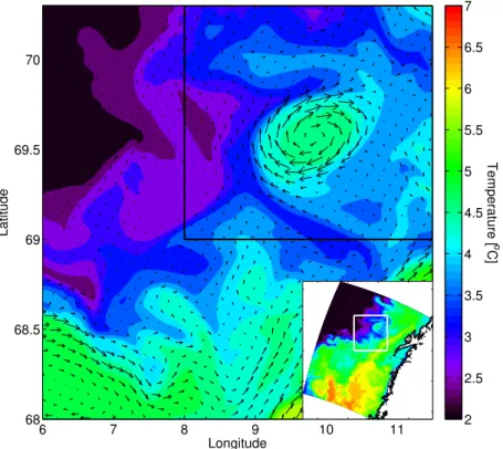
Fig. 1.Surface temperature and currents in the area of the eddy on 21 March 1999, which is the initial day of the particle simulation. The eddy is at this point fairly isolated from other mesoscale activity in the area. The particles at depth were released within the area shown, while the black rectangle indicate the initial area covered by the surface particles. Inserted: The surface temperature of the entire model domain, the white rectangle indicates the area shown in the large figure.
activity. We performed 5 different experiments with released particles, as summarized in Table 1. First, surface particles were released in a square area covering the eddy (8◦E– 11◦30′E and 69◦N–70◦18′N–Fig. 1) on March 21 and fol-lowed for 20 days. Second, particles at depth were released in a larger area (6◦
E–11◦ 30′
E, and 68◦ N–71◦
18′
N–Fig. 1) and followed for 30 days. The initial distribution was uni-form both in the horizontal and vertical. In the surface ex-periment 50 000 plankton/food particles were released in the upper 100 m of the eddy while 100 000 particles, represent-ing the mesopelagic fish/deep scatterrepresent-ing layer, were released between 600 and 800 m. All the particles were released si-multaneously on the fist day of the simulations. In the upper water column three experiments were performed: (i) the par-ticles follow the three-dimensional current field; (ii) they are held at a constant depth; and (iii) they perform DVM. The DVM is set to 100 m, which we considered an upper limit for small organisms. The DVM was configured by initiating a downward migration at 6 a.m. and an upward migration at 6 p.m. The particles move with a speed of 20 m h−1and thus use 5 h to cover the 100 m migration. The DVM occurs uni-formly across the domain. In the deeper layers two experi-ments were performed; one where the particles were kept at constant depth and the second where they followed the three-dimensional current field (Table 1).
2.3 Physical quantities
In order to relate the particle distribution from the simula-tions to the dynamics of the eddy we use the physical quan-tities vorticity, divergence, vertical velocity and the Okubo-Weiss parameter. Vorticity (ζ )describes the waters tendency to rotate and is expressed mathematically as
ζ =∂v
∂x− ∂u ∂y
Divergence (D) is the tendency of the water to diverge or con-verge (negative dicon-vergence) and is described mathematically
D=∂u
∂x+ ∂v ∂y
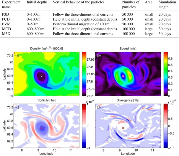
Table 1.Summarizing the 5 different experiments performed with released particles.
Experiment Initial depths Vertical behavior of the particles Number of Area Simulation
name particles length
P3D 0–100 m Follow the three-dimensional currents 50 000 small 20 days
PCD 0–100 m Held at the initial depth (constant depth) 50 000 small 20 days
PVM 0–50 m Perform diurnal migration of 100 m 50 000 small 20 days
MCD 600–800 m Held at the initial depth (constant depth) 100 000 large 30 days
M3D 600–800 m Follow the three-dimensional currents 100 000 large 30 days
Fig. 2.The physical properties of the eddy. The eddy is almost circular with a small “tail” and, being an anticyclone, has lower density at
the center(a). The maximum speed is found around the rim(b), and in the same area the boundary between the core with negative vorticity
and the outer part with positive vorticity is found(c). The divergence field(d)is strongest in the outer part of the eddy where there is strong
convergence, in addition we find an area with convergence adjacent to an area with divergence in the “tail”. All field have been taken from layer 5 (from 16 to 21 m) of the model on 31 March 1999. The eddy center has been marked with an “x”.
The Okubo-Weiss parameter, W, (Weiss, 1991; Okubo, 1970) is defined as follows:
W=
∂u
∂x− ∂v ∂y
| {z }
normalstrain 2+
∂v
∂x+ ∂u ∂y
| {z }
shearstrain 2−
∂v
∂x− ∂u ∂y
| {z }
vorticity 2
The Okubo-Weiss parameter is an aid in identifying vorticity-dominant (W <0) and strain-dominated regions (W >0). Very little exchange is expected to occur across the boundary between these two regions. Moreover, intense stir-ring and exchange processes with the background field may take place in the strain-dominated region (Isern-Fontanet et al., 2004). In the strictest sense the Okubo-Weiss parameter is only applicable to 2-D turbulence, but can also be applied to 3-D fields provided the divergence is moderately weak.
3 Simulation results
3.1 Physical evolution of the eddy
L
a
ti
tu
d
e
[
o N
]
Longitude [o E ]
V ertical velocity [m/day]
model layer 5
(a)
8 8.5 9 9.5 10 10.5
69 69.5 70 70.5
10 5 0 5 10
Longitude [o E ]
model layer 15
(b)
8 8.5 9 9.5 10 10.5 20
10 0 10 20
Latitude [o N]
D
e
p
th
[
m
]
(c)
69 69.5 70 70.5
1000 800 600 400 200 0
20 10 0 10 20
Longitude [o E ]
(d)
8 8.5 9 9.5 10 10.5 20
10 0 10 20
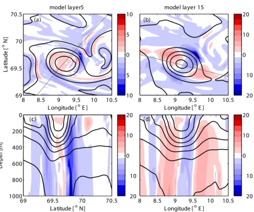
Fig. 3.The vertical velocity in the eddy, close to the surface in layer 5 (16–21 m)(a), and further down in layer 15 (152–178 m)(b). Two
cross-sections of the vertical velocity in the eddy are shown (candd), the location of each cross-section is shown with a gray thin line in the
panel above. The thick black lines are isopycnals. The vertical velocity and density are 5-day averages from the period 19–23 March 1999.
along the edge. The highest vorticity coincided with the two zones of maximum orbital motion.
The divergence pattern, on the other hand, was less dis-tinct, with alternating bands of divergence and convergence in the same area where positive vorticity was found (Fig. 2). The mean divergence over 20 days (not shown) also shows two patches of high convergence on either side of the eddy, and these areas of high convergence stayed fixed in space relative to the eddy. The corresponding vertical velocity in the upper layers of the eddy was upwards in the center and downwards in two bands around the outer rim (Fig. 3). Since these bands revolve with the eddy, the mean vertical velocity over 20 days is uniform around the eddy with upwelling in the eddy center and downwelling along the rim. In particular the regions of downward velocity coincided with regions of strong convergence (Fig. 2). With depth, the vertical veloc-ities increased and alternated between positive and negative velocity on either side of the eddy center. The Okubo-Weiss parameter suggests that the eddy was vorticity dominated in the core and strain dominated in a ring around the core (Fig. 4). The relation between the Okubo-Weiss parameter and particle distribution will be discussed in Sect. 3.2.
The hydrodynamic structure of the eddy gradually weak-ened throughout the simulation period; e.g. the maximum
surface speed decreased from 0.64 m s−1to 0.54 m s−1over 20 days, and the deep isopycnals in the center shoaled, i.e. the 1028.01 kg m−3isopycnal shoaled from 894 m on March 21 to 851 m on April 10. During the 20 days the eddy moved roughly 25 km towards the southwest.
3.2 Surface particle simulations
69 69.5 70
Latitude
day 9 P3D + vorticity
day 19 P3D + vorticity
69 69.5 70
Latitude
PCD + divergence PCD + divergence
8 9 10 11 69
69.5 70
Longitude
Latitude
PVM + Okubo−Weiss
8 9 10 11 Longitude PVM + Okubo−Weiss
Number of particles
2 4 6 8 10 12 14 16 18 20 22
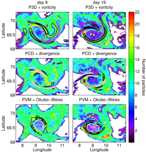
Fig. 4.Depth-integrated particle concentration for each of the surface particle simulations on day 9 (1st column) and day 19 (2nd col-umn) after initialization. The colour show the number of particles within a pixel, white pixels have no particles (the raw fields were filtered
with a 3×3 median filter to make patterns more visible). Particles at all depth were taken into account and the size of the pixels are
1/48◦×1/19.2◦. The overall pattern of distribution is similar for all three runs. Super-imposed on the particle concentrations are physical
parameters in model layer 5 plotted as contours – black for positive values and pink for negative values: Upper panel – vorticity (contour
in-tervals: 2×10⁻⁵s−1), middle panel – divergence (contour intervals: 5×10⁻⁶s−1), and lower panel – the Okubo-Weiss parameter (contour
intervals: 1×10⁻⁹s−2).
in areas with positive Okubo-Weiss parameter (i.e. strain dominated regions), but there is not a one-to-one corre-spondence between positive Okubo-Weiss and high particle concentration (Fig. 4).
The particle aggregation along the eddy rim occurred in all three simulations, but the highest particle concentrations were reached in the run with constant depth in the water col-umn (PCD). In the P3D-run the particles were also trans-ported downward along the rim of the eddy. This downward movement was confined to the two bands on either side of the eddy center collocated with the maximum orbital motion and vorticity. Moreover, in all the three runs the upper and inner part of the eddy was gradually emptied for particles. Towards the end of the simulation period the particles were largely ab-sent to the south of the eddy, while they were still abundant to the north because the mean current in the area was north-wards. Around the eddy periphery, however, the highest par-ticle concentrations were found to the southwest of the eddy
center immediately adjacent to a region outside the eddy that was completely free of particles (Fig. 3).
In all three simulations another patch of high particle con-centration occurred outside the eddy on the southeast side (Fig. 4). These particles originated from a patch originally accumulated at the eddy rim that suddenly separated from the eddy around 10 days into the simulation. Whether this is a result of internal eddy dynamics or some external forcing is unclear, but the local wind field applied as forcing did not reveal anything unusual, such as particularly strong winds, in that period.
7.5 8 8.5 9 9.5 10 10.5 11 11.5 69
69.5 70 70.5
Longitude
Latitude
Vorticity [1/s]
−1.5 −1 −0.5 0 0.5 1 1.5 x 10⁻⁴
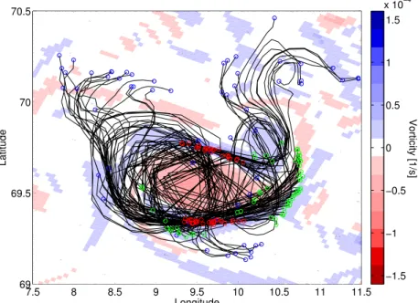
Fig. 5.Surface particle trajectories for a subset the particles that were aggregated in the high-vorticity region after 4 days of simulation. The trajectories are shown on top of the vorticity field on the same day in model layer 5 (16–21 m). Green circles indicate the initial position, red circles indicate the position on day 4, and blue circles indicate the final position after 20 days. The straight lines in some of the trajectories occur because the particle positions were only saved every 24 h.
same particles, but that these patches are continuously ag-gregated as the eddy moves. The particles that originated in the center, on the other hand, tended to stay within the eddy, although the inner ones gradually moved towards the eddy periphery without crossing into the positive vorticity regions. This caused additional increase in the concentration of par-ticles around the eddy rim. In contrast to the parpar-ticles that ended up in the high-vorticity regions, very few of the parti-cles that originated in the center became detached from the eddy. From a subsample of particles we estimated that 88 % of the particles starting in the eddy center stayed inside the eddy throughout the 20-day simulation. The ones that exited the center did so through the negative-vorticity “tail” seen on Fig. 4 or Fig. 2, reflecting the reluctance of particles to cross vorticity gradients.
3.3 Particle simulation at depth
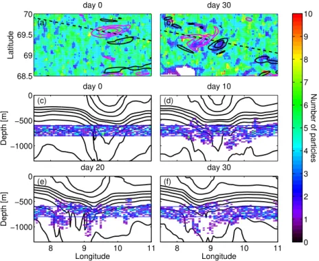
In the simulation with particles between 600 and 800 m the horizontal distribution stayed fairly uniform as the strongest convergence and divergence occurred close to the surface. In the run with constant vertical distribution there was no difference in the particle concentration in any area in or around the eddy, even after 30 days (Fig. 6). In the run where the particles were allowed to move with the vertical currents, particles were transported vertically, although the depth-integrated horizontal particle distribution stayed fairly constant. After about 10 days particles close to the rim of the eddy had moved 100–200 m both upwards and downwards
(Fig. 6). In accordance with the vertical velocity at depth (Fig. 3), the vertical motion was initially asymmetric with re-spect to the eddy, but as the eddy revolved the distribution be-came more symmetric. The particles allowed to move verti-cally appeared to follow the isopycnals at the rim of the eddy (deepening towards the eddy center), while particles released in the eddy centre moved upwards, creating an empty, bowl-shape region at the eddy center between 800 and 1000 m after 30 days (Fig. 6).
4 Discussion
4.1 Particle dispersion
68.5 69 69.5 70
Latitude
day 0
(a)
day 30
(b)
Depth [m]
day 0
(c)
−1000 −500 0
day 10
(d)
Longitude
Depth [m]
day 20
(e)
8 9 10 11
−1000 −500 0
Longitude day 30
(f)
8 9 10 11
Number of particles
0 1 2 3 4 5 6 7 8 9 10
Fig. 6.The two upper panels show depth-integrated horizontal distribution of particles in experiment M3D on(a)day 0 and(b)day 30. The
contours show vorticity in model layer 21 (depth: 437–616 m), contour intervals are 1×10⁻⁵s−1and pink is negative and black positive
vorticity. The lower 4 panels show vertical distribution of particles along a section through the middle of the eddy on day(c)0(d)10,(e)20,
and(f)30. All particles in experiment M3D that were within 5 km of the section were counted and the size of the pixels is 20 m×2.6 km.
The black contour lines in(c)–(f)are isopycnals. Since the eddy moves throughout the simulation, the position of the section followed the
eddy, the positions of the section on day 0 and 30 are shown in(a)and(b)respectively.
moved horizontally, and some performed diurnal vertical mi-gration (Table 1). The main result for the surface distribution was largely the same; the eddy center was gradually emptied of particles, while areas around the rim of the eddy attained high concentrations (Fig. 4). The vertical motion of the par-ticles played a lesser role; although the parpar-ticles that stay at a constant depth attain higher concentrations in terms of par-ticles per volume because they cannot move up or down, the depth-integrated concentration were not significantly differ-ent (Fig. 4). Particles released between 600 and 800 m were either kept at constant depth or followed the 3-D model ve-locity (Table 1). In contrast to the surface simulations, the depth-integrated number of particles stayed uniform through-out the simulation period, but when the particles were al-lowed to move vertically (M3D), an evolution where the par-ticles gradually align along the isopycnals was seen. This created an empty area between two layers of particles at the eddy center (Fig. 6). All the particles that ended up in the deepest part of the eddy originated on the western side of the eddy, probably pushed down with the thermocline as the eddy moved southwestward.
At the surface, the highest concentration of particles was associated with high positive vorticity. The particle trajec-tories revealed that the particles in these high-concentration patches originated outside the eddy (Fig. 5), and, contrary to
what we expected in a region where particles appear to ag-gregate, there was a high exchange of particles between the high-concentration patch and the surrounding area in these regions. The particles originating in the core of the eddy gradually moved outwards during the simulation thus in-creasing the particle concentration along the eddy rim and gradually emptying the center. Only a few of these particles detached from the eddy during the simulation and only ex-ited through the negative vorticity “tail” of the eddy (Fig. 2), reflecting that the vorticity gradient along the rim of the an-ticyclonic eddy acts as barrier for the continuous outward spreading of the particles (Priovenzale, 1999). According to Provenzale (1999), regions with positive W (i.e. strain-dominated regions) have local exponential divergence of nearby particles, while particles in regions with negative W (vorticity-dominated) stay at the same distance from each other. This agrees with the difference in behavior of the parti-cles in the different regions of the eddy studied here, although Provenzale (1999) considers idealized barotropic flow.
4.2 Limitations
the the particle distribution and concentration. In so doing an eddy that was fairly isolated from other mesoscale processes was chosen. However, in other realistic simulations it may be possible to find eddies that is almost completely isolated, for instance warm/cold core rings in the Gulf Stream. Although isolated eddies are not uncommon in the ocean, it is more common that they occur in eddy-rich areas, with enhanced likelihood of eddy-eddy interaction. An isolated eddy was chosen here to simplify the analysis, but we expect that the results presented here will aid the analysis of more complete eddy fields in future studies. Ideally it would also be inter-esting to investigate the effect of a cyclonic eddy on particle distribution, but the eddy field in the model revealed that the cyclonic eddies, although they occurred quite often, are not very stable and tend to be pulled out into elongated filaments after only a few days. This has also been seen in other mod-eling studies and is a result of weakening of cyclones result-ing from strain deformation induced by vortex Rossby waves (Koszalka et al., 2009; Graves et al., 2006).
The vertical velocity (Fig. 3) plays a major role in dis-tributing the particles both at the surface and at depth, but as long as direct observations of the vertical velocities in ocean eddies are rare, the representativeness of the simulated verti-cal motion remain unknown. The method used for verti- calculat-ing vertical velocity in the model (see Sect. 2.3) avoids the accumulation of errors that can occur when integrating the continuity equation to obtain the vertical velocity.
The number of particles is limited by computational re-sources, and with 50 000–100 000 particles over an area of O(104)km2we come nowhere close to the actual number of non-swimming organisms they are meant to represent. For example,Calanus finmarchius, the dominant copepod of the Norwegian Sea, has typical concentrations of O(104–105)
individuals/m2 (Samuelsen et al., 2009; Edvardsen et al., 2006). However, experiments with fewer particles showed little difference in the overall results with respect to the hor-izontal distribution and increasing the number of particles would not make a difference unless we also increase the hor-izontal resolution of the physical model. For the vertical dis-tribution it is clear that there would be an advantage with more particles, particularly when attempting to represent a section through the eddy (Fig. 6).
Other aspects of “real life” complicate this picture. Most eddies have a temperature difference with the surrounding water and temperature affect the growth of most organism from plankton to fish larvae. A simple numerical exercise (results not shown) showed that if you have a warm eddy in an area with uniform zooplankton concentration, this would lead to increased zooplankton biomass, granted that the zoo-plankton growth is not food-limited, because of the tempera-ture effect on the growth. If on the other hand the zooplank-ton biomass is redistributed into high-concentration areas, they may become food limited and this can lead to a reduc-tion in the total biomass. In addireduc-tion, eddies may increase or decrease the primary production in an area by modifying
the vertical nutrient transport to the surface. This would af-fect the local production and food availability as well. Fish and marine mammal often have preferences for depth, tem-perature and salinity, and may either avoid or seek the eddy depending on their particular preference. Detritus and fe-cal pellets can have sinking velocities ranging from 10 to 100 m d−1, since this is of the same order of magnitude than the vertical velocities found in the eddy, this may lead to increased concentration of dead particles in the upwelling parts of the eddy. Probably the effect will be largest on slow-sinking detritus, since particles with vertical slow-sinking speed of
∼O(100 m d−1) will sink below the eddy in just a few days.
The next step in our research will be to investigate these as-pect using an individual based model for zooplankton (Hjøllo et al., 2012) rather than simple particles.
4.3 Model – observation comparison
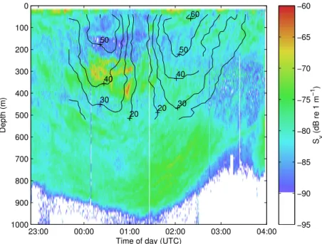
The setup of the numerical experiments were originally in-spired by the observed distributions of biomass in anticy-clonic eddies observed in the field (Fig. 7), the details of these surveys are given in Godø et al. (2012). Specifically an anticyclonic eddy in the Lofoten Basin region in Novem-ber 2009 showed increased concentration of biomass (specif-ically krill) at the surface close to the rim of the eddy. At depth, the layer of mesopelagic fish had been displaced sev-eral hundred meters downwards (Fig. 7) apparently follow-ing the isotherms. The numerical experiment was set up in order to investigate whether the hydrodynamic conditions in the eddy could explain some of these observations of ac-cumulated biomass and whether the vertical positioning of organisms played a role.
50
40
30
60
50
40
30 20 20 50
40
30
60
50
40
30 20 20
Time of day (UTC)
Depth (m)
20 20
30 40
50 60
30 40 50
23:00 00:00 01:00 02:00 03:00 04:00
0
100
200
300
400
500
600
700
800
900
1000
Sv
(dB re 1 m
−1
)
−95 −90 −85 −80 −75 −70 −65 −60
Fig. 7.An example of the acoustic signature of an anticyclone recorded in the Lofoten basin during November 2009 while crossing the eddy from west to east. The edges of the eddy were crossed at about 23:30 and 03:00 and the center between 01:00 and 01:30. The echogram shows mean volume backscattering strength (Sv, an indication of organism spatial density and hence of biomass). Higher Sv values indicate
higher density. Black contour lines show absolute velocity in cm s−1. Note the higher concentrations of biomass in the surface layer close to
the edges (<50 m around 23:30, 02:00, and 03:00) and the empty centre from the surface to 200 m depth.
The relationship between mesoscale eddies and biomass has also been investigated in other regions. Sabarros et al. (2009) found high concentration of micronekton at the periphery of the eddies, similar to the finding in Godø et al. (2012). While Yebra et al. (2009) and (Holliday et al., 2011) found high biological concentration associated with anticyclonic eddies in the Labrador Sea and off Australia respectively, but no evidence of higher concentration at the eddy rim. The differences could be caused by different eddy dynamics, different stages in the development of the eddy (Bakun, 2006), or differences in the biological organ-isms present, but more field measurements are necessary to understand the eddy-ecosystem interactions.
Aggregation of particles, as seen in the model simulations, may affect the overall distribution and amount of biomass in relation to mesoscale activity. If we assume that the particles in the simulation represent slow-swimming zooplankton it is conceivable that the high-concentration patches will attract higher trophic levels such as fish and sea birds. One could imagine that swimming fish could just stay in this area and wait for food to come along. On the other hand if the zoo-plankton are aggregated, their growth may become food lim-ited and after some time the aggregation areas may no longer be attractive to predators. The model showed that there were dynamic differences within regions with high particle con-centration. Some regions had a very high exchange of parti-cles and it is not likely that these organisms would experience
any food limitation as they are quickly transported away from the area. In other patches there were little exchange with the surroundings and it is more likely that these will experience food shortage, but this of course also depend on the local primary production.
5 Conclusions
Whether this increase in biomass at depth could be connected to the physical accumulation processes at the surface is an open question.
Supplementary material related to this article is
available online at: http://www.ocean-sci.net/8/389/2012/ os-8-389-2012-supplement.zip.
Acknowledgements. This work was supported by the RCN ”Havet
og Kysten” project AcuSat – 19026I/S40. Many thanks to Gavin John Macaulay for preparing Fig. 7, and to J. Skardhamar, H. Søiland and the two anonymous reviewers for valuable comments on the manuscript. A grant of computer time from the NOTUR Project has also been used.
Edited by: M. Hecht
References
Andersson, M., Orvik, K. A., LaCasce, J. H., Koszalka, I., and Mau-ritzen, C.: Variability of the Norwegian Atlantic Current and as-sociated eddy field from surface drifters, J. Geophys. Res., 116, C08032, doi:10.1029/2011JC007078, 2011.
Bakun, A.: Fronts and eddies as key structures in the habitat of ma-rine fish larvae: Opportunity, adaptive response and competitive advantage, Sci. Mar., 70, 105–122, 2006.
Benitez-Nelson, C. R., Bidigare, R. R., Dickey, T. D., Landry, M. R., Leonard, C. L., Brown, S. L., Nencioli, F., Rii, Y. M., Maiti, K., Becker, J. W., Bibby, T. S., Black, W., Cai, W. J., Carlson, C. A., Chen, F. Z., Kuwahara, V. S., Mahaffey, C., McAndrew, P. M., Quay, P. D., Rappe, M. S., Selph, K. E., Simmons, M. P., and Yang, E. J.: Mesoscale eddies drive increased silica export in the subtropical Pacific Ocean, Science, 316, 1017–1021, 2007. Bertino, L. and Lisæter, K. A.: The TOPAZ monitoring and
predic-tion system for the Atlantic and Arctic Oceans, Journal of Oper-ational Oceanography, 1, 15–18, 2008.
Bleck, R.: An oceanic general circulation model framed in hybrid isopycnic-cartesian coordinates, Ocean Model., 4, 55–88, 2002. Carnes, M. R.: Description and evaluation of GDEM-V 3.0 Stennis
Space Center, Technical report, NRL/MR/7330–09-9165, Sten-nis, USA , 2009.
Cushing, D. H.: The vertical migration of planktonic crustacea, Biol. Rev., 26, 158–192, 1951.
Dale, T. and Kaartvedt, S.: Diel patterns in stage-specific vertical
migration ofCalanus finmarchicusin habitats with midnight sun,
Ices J. Mar. Sci., 57, 1800–1818, 2000.
Edvardsen, A., Pedersen, J. M., Slagstad, D., Semenova, T., and
Ti-monin, A.: Distribution of overwinteringCalanusin the North
Norwegian Sea, Ocean Sci., 2, 87–96, doi:10.5194/os-2-87-2006, 2006.
Frajka-Williams, E., Rhines, P. B., and Eriksen, C. C.: Physical con-trols and mesoscale variability in the Labrador Sea spring phyto-plankton bloom observed by seaglider, Deep-Sea Res. Pt. I, 56, 2144–2161, 2009.
Garraffo, Z. D., Mariano, A. J., Griffa, A., Veneziani, C., and Chas-signet, E. P.: Lagrangian data in a high-resolution numerical sim-ulation of the North Atlantic I. Comparison with in situ drifter data, J. Mar. Syst., 29, 157–176, 2001.
Gascard, J.-C. and Mork, K. A.: Climatic Importance of large-scale and mesoscale circulation in the Lofoten Basin Deduced from Lagrangian observations, in: Arctic-Subarctic Ocean Fluxes, edited by: Dickson, R. R., Meincke, J., and Rhines, P., Springer, Dordrecht, 131–143, 2008.
Genin, A., Jaffe, J. S., Reef, R., Richter, C., and Franks, P. J. S.: Swimming against the flow: A mechanism of zooplankton ag-gregation, Science, 308, 860–862, 2005.
Godø, O. R., Samuelsen, A., Macaulay, G. J., Patel, R., Hjøllo, S. S. t., Horne, J., Kaartvedt, S., and Johannessen, J. A.: Mesoscale eddies are oases for higher trophic marine life, PLoS ONE, 7, e30161, 2012.
Graves, L. P., McWilliams, J. C., and Montgomery, M. T.: Vor-tex evolution due to straining: A mechanism for dominance of strong, interior anticyclones, Geophys. Astro. Fluid, 100, 151– 183, 2006.
Hansen, C., Kvaleberg, E., and Samuelsen, A.: Anticyclonic eddies in the Norwegian Sea; their generation, evolution and impact on primary production, Deep-Sea Res. Pt. I, 57, 1079–1091, 2010. Hjøllo, S. S., Huse, G., Skogen, M. D., and Melle, W.: Modeling
secondary production in the Norwegian Sea with a fully
cou-pled physical/primary production/individual-basedCalanus
fin-marchicusmodel system, Mar. Biol. Res., 8, 508–526, 2012.
Holliday, D., Beckley, L. E., and Olivar, M. P.: Incorporation of larval fishes into a developing anti-cyclonic eddy of the Leeuwin Current off south-western Australia, J. Plankton Res., 33, 1696– 1708, 2011.
Isern-Fontanet, J., Font, J., Garcia-Ladona, E., Emelianov, M., Mil-lot, C., and Taupier-Letage, I.: Spatial structure of anticyclonic eddies in the Algerian Basin (Mediterranean Sea) analyzed using the Okubo-Weiss parameter, Deep-Sea Res. Pt. I, 51, 3009–3028, doi:10.1016/J.Dsr2.2004.09.013, 2004.
Klein, P. and Lapeyre, G.: The oceanic vertical pump induced by mesoscale and submesoscale turbulence, Ann. Rev. Mar. Sci., 1, 351–375, doi:10.1146/annurev.marine.010908.163704, 2009. Koszalka, I., Bracco, A., McWilliams, J. C., and
Proven-zale, A.: Dynamics of wind-forced coherent
anticy-clones in the open ocean, J. Geophys. Res., 114, C08011, doi:10.1029/2009jc005388, 2009.
Luck, D. G. and Pietsch, T. W.: In-situ observations of a
deep-sea ceratioid anglerfish of the genus oneirodes (lophiiformes:
Oneirodidae), Copeia, 2008, 446–451, doi:10.1643/ce-07-075, 2008.
Lyard, F., Lefevre, F., Letellier, T., and Francis, O.: Modelling the global ocean tides: Modern insights from FES2004, Ocean Dyn., 56, 394–415, doi:10.1007/s10236-006-0086-x, 2006.
Mahadevan, A. and Archer, D.: Modeling the impact of fronts and mesoscale circulation on the nutrient supply and biogeochem-istry of the upper ocean, J. Geophys. Res.-Oceans, 105, 1209– 1225, 2000.
McGillicuddy, D. J. and Robinson, A. R.: Eddy-induced nutrient supply and new production in the Sargasso Sea, Deep-Sea Res. Pt. I, 44, 1427–1450, 1997.
P. G., Goldthwait, S. A., Hansell, D. A., Jenkins, W. J., Johnson, R., Kosnyrev, V. K., Ledwell, J. R., Li, Q. P., Siegel, D. A., and Steinberg, D. K.: Eddy/wind interactions stimulate extraordinary mid-ocean plankton blooms, Science, 316, 1021–1026, 2007. Neilson, J. D. and Perry, R. I.: Diel vertical migrations of marine
fishes - an obligate or facultative process, Adv. Mar. Biol., 26, 115–168, 1990.
Oki, T. and Sud, Y. C.: Design of total runoff integrating pathways (TRIP) – a global river channel network, Earth Interact., 2, 1–37, 1998.
Okubo, A.: Horizontal dispersion of floatable particles in the vicin-ity of velocvicin-ity singularities such as convergences, Deep-Sea Res., 17, 445–454, 1970.
Olson, D. B., Hitchcock, G. L., Mariano, A. J., Ashjian, C. J., Peng, G., Nero, R. W., and Podesta, G. P.: Life on the edge: Marine life at fronts,, Oceanography, 7, 52–60, 1994.
Pearcy, W. G., Krygier, E. E., and Cutshall, N. H.: Biological trans-port of zinc-65 into the deep sea, Limnol. Oceanogr., 22, 846– 855, 1977.
Provenzale, A.: Transport by coherent barotropic vortices, Annu. Rev. Fluid Mech., 31, 55–93, doi:10.1146/annurev.fluid.31.1.55, 1999.
M´enard, F., L´ev´enez, J. J., Tew-Kai, E., and Ternon, J. F.: Mesoscale eddies influence distribution and aggregation patterns of mi-cronekton in the Mozambique Channel, Mar. Ecol. Prog. Ser., 395, 101–107, 2009.
Samuelsen, A. and Hjøllo, S. S.: Physical model development and validation in the acusat project, Nansen Environmental and Re-mote Sensing Center, Bergen, 2011.
Samuelsen, A., Huse, G., and Hansen, C.: Shelf recruitment of
Calanus finmarchicusoff the west coast of norway: Role of
phys-ical processes and timing of diapause termination, Mar. Ecol. Prog. Ser., 386, 163–180, doi:10.3354/meps08060, 2009. Simmons, A. S., Uppala, D. D., and Kobayashi, S.: ERA-interim:
New ECMWF reanalysis products from 1989 onwards, in: Newsletter, ECMWF, Newsletter 110 – Winter 2006/2007, 11 pp., 2007.
Weiss, J.: The dynamics of enstrophy transfer in two-dimensional hydrodynamics, Physica D: Nonlinear Phenomena, 48, 273–294, 1991.