www.atmos-chem-phys.net/14/7929/2014/ doi:10.5194/acp-14-7929-2014
© Author(s) 2014. CC Attribution 3.0 License.
An evaluation of ozone dry deposition simulations in East Asia
R. J. Park1, S. K. Hong1, H.-A. Kwon1, S. Kim2, A. Guenther3, J.-H. Woo4, and C. P. Loughner5
1School of Earth and Environmental Sciences, Seoul National University, Seoul, Korea 2Department of Earth System Science, University of California, Irvine, CA, USA 3Pacific Northwest National Laboratory, Richland, WA, USA
4Department of Environmental Engineering, Konkuk University, Seoul, Korea
5CMNS-Earth System Science Interdisciplinary Center, University of Maryland, College Park, MD, USA Correspondence to:R. J. Park ([email protected])
Received: 2 December 2013 – Published in Atmos. Chem. Phys. Discuss.: 13 January 2014 Revised: 31 May 2014 – Accepted: 29 June 2014 – Published: 11 August 2014
Abstract. We use a 3-D regional atmospheric chemistry transport model (WRF-Chem) to examine ozone dry depo-sition in East Asia, which is an important but uncertain re-search area because of insufficient observation and numerical studies focusing on East Asia. Here we compare two widely used dry deposition parameterization schemes, the Wesely and M3DRY schemes, which are used in the WRF-Chem and Community Multiscale Air Quality (CMAQ) models, re-spectively. Simulated ozone dry deposition velocities with the two schemes under identical meteorological conditions show considerable differences (a factor of 2) owing to surface resistance parameterization discrepancies. Resulting ozone concentrations differ by up to 10 ppbv for a monthly mean in May when the peak ozone typically occurs in East Asia. An evaluation of the simulated dry deposition velocities shows that the Wesely scheme calculates values with more pro-nounced diurnal variation than the M3DRY and results in a good agreement with the observations. However, we find sig-nificant changes in simulated ozone concentrations using the Wesely scheme but with different surface type data sets, in-dicating the high sensitivity of ozone deposition calculations to the input data. The need is high for observations to con-strain the dry deposition parameterization and its input data to improve the use of air quality models for East Asia.
1 Introduction
Ozone (O3)is a harmful air pollutant in surface air and the
primary chemical oxidation driver in the free troposphere. Tropospheric ozone concentrations are largely controlled by
the balance among net chemical production, influx from the stratosphere, and physical losses (Wu et al., 2007). Dry de-position of ozone is a dominant physical loss process and accounts for approximately 25 % of the total ozone lost in the troposphere (Lelieveld and Dentener, 2000).
In typical chemical transport models, dry deposition is cal-culated as a first-order process that uses dry deposition ve-locity, which is parameterized as a function of surface type and atmospheric stability conditions (Wesely, 1989). How-ever, in models, its parameterization is highly uncertain be-cause of complexities from surface conditions at sub-grid scales (Wu et al., 2011). Thus, previous studies on dry de-position calculations have primarily focused on the United States and Europe, for which observations on ozone fluxes or dry deposition velocities were available to validate either simulated ozone losses or dry deposition velocity parameter-ization (Rannik et al., 2012; Wu et al., 2011; Charusombat et al., 2010; Gerosa et al., 2007).
simulation is important for accurately assessing the contribu-tion from a source to regional air pollutant concentracontribu-tions.
However, air quality model evaluations have been rela-tively limited because of the lack of long-term regional ob-servations in East Asia. In particular, evaluating individual processes, including the dry deposition calculation, has not been rigorous for East Asia. Several studies focusing on ozone dry deposition simulations have been conducted for a tropical forest in Southeast Asia (Matsuda et al., 2005, 2006), but the vegetation type differs from East Asia.
The purpose of this study is to evaluate the ozone dry de-position simulations (schemes) in two of the most widely used regional air chemistry models in East Asia: the Weather Research and Forecasting-Chemistry (WRF-Chem) and the Community Multiscale Air Quality (CMAQ) models. We conducted multiple model simulations to understand the dif-ferences between the two models as well as the two different dry deposition schemes and factors that affect dry deposition and ozone concentrations in East Asia. We also evaluated the simulated ozone concentration and dry deposition veloc-ity by comparing such results with observations. Finally, we conducted several sensitivity simulations using different in-put data sets to demonstrate the uncertainties of the dry depo-sition calculations, which should be considered in assessing the spatial and temporal distributions of ozone and the contri-butions from a specific source to a particular region, includ-ing the trans-boundary transport of ozone precursors in East Asia.
2 Model description 2.1 General description
We used the WRF-Chem model (version 3.3) to simu-late ozone in East Asia. The model is a fully coupled meteorology–chemistry model, which was developed by the National Center for Atmospheric Research (NCAR) (Grell et al., 2005) to account for the interaction between meteorolog-ical and chemmeteorolog-ical processes at each time step (Chapman et al., 2009). The model is described in detail elsewhere (Grell et al., 2005). Herein we primarily describe our model simu-lations.
The model has a horizontal resolution of 45×45 km with
14 eta vertical grids and a 50 hPa top. The model domain for our simulations is shown in Fig. 1, which includes the nested grid domain that focuses on the Korean peninsula. For mete-orology simulations, we used physics modules in the WRF, as shown in Table 1. In particular, turbulent mixing at the surface and within the planetary boundary layers was calcu-lated using schemes developed by Chen and Dudhia (2001) and Hong et al. (2006), respectively.
We used anthropogenic emissions from the Sparse Ma-trix Operator Kernel Emissions-Asia (SMOKE-Asia), which was developed by Woo et al. (2012) to operate the CMAQ
Table 1.Model set-up for the WRF-Chem simulations.
Feature Selected configuration
Domain East Asia on 45 km grid with 14 layers
Domain top 50 hPa
Emission SMOKE-Asia (only anthropogenic) Long wave radiation RRTM
Short wave radiation Goddard Microphysics Lin (Purdue) Cumulus parameterization Grell–Devenyi Vertical diffusion Eddy Chemical mechanism CBMZ Surface layer physics Monin–Obukhov Land surface model Noah
Planetary boundary layer YSU
Photolysis Fast-J
Table 2.Species mapping between the CB05 and CBMZ chemical schemes.
CBMZ CB05 CBMZ CB05 (WRF-Chem)
E_ALD ALD2+ALDX E_TOL TOL E_CO CO E_XYL XYL E_OL2 ETH E_ETH ETHA E_HCHO FORM E_C2H5OH ETOH E_ISOP ISOP E_OLI IOLE E_NH3 NH3 E_CH3OH MEOH
E_NO NO NASN
E_NO2 NO2 TERP
E_OLE OLE E_KET E_PAR PAR E_ORA2 E_SO2 SO2 E_CLS
∗NASN, TERP, E_KET, E_ORA2, and E_CLS have no corresponding species.
model (Byun and Ching, 1999) over East Asia. The SMOKE-Asia calculates anthropogenic emissions based on the carbon bond 05 (CB05) chemical mechanism (Appel et al., 2007), which slightly differs from the carbon bond mechanism Z (CBMZ) used in WRF-Chem. We used the chemical map-ping in Table 2 to match the emission species between CB05 and CBMZ. A few species do not precisely correspond be-tween the two schemes, but such species are relatively unim-portant for our ozone simulations below. The total NOx, CO,
and volatile organic compound (VOC) emissions in the do-main are 24.6, 150.2, and 96.0 Tg yr−1, respectively.
The initial and lateral boundary conditions for the me-teorology simulations were determined using a WRF pre-processing system with the NCEP Final Operational Model Global Tropospheric Analyses data (National Centers for En-vironmental Prediction, 2000). Climatological values were used to generate the initial and boundary values for the chem-ical species concentrations (Grell et al., 2005).
Figure 1.Monthly mean O3dry deposition velocities in East Asia for May 2004 from WRF-Chem using the Wesely scheme (left) and the
M3DRY scheme (middle). The differences between the two simulations are shown in the right panel.
provided in Sects. 2.2 and 2.3. Identical boundary and initial conditions were used for the model, including species emis-sions, except for the dry deposition scheme. Therefore, the differences in the results are entirely due to the discrepancy between the two dry deposition schemes. The model simula-tion for April was used for spin-up, and we primarily focus our analysis on the results for May, when the peak ozone typically occurs in East Asia. Because of summer monsoon, ozone concentrations are lower in summer than in spring in East Asia (Li et al., 2007).
2.2 Dry deposition parameterization
Chemical species loss (F) owing to dry deposition in air chemistry models is typically computed as a first-order pro-cess with the dry deposition velocity as shown in Eq. (1).
F =vdC (1)
vdindicates the dry deposition velocity, andCrepresents the
species concentrations in the lowest model layer. Therefore, the species lost through dry deposition is directly propor-tional to the dry deposition velocity, which is parameterized in such models.
The dry deposition velocity is computed as the reciprocal of the sum for aerodynamic resistance (Ra), quasi-laminar
resistance (Rb), and surface resistance (Rc)as follows:
vd= 1
Ra+Rb+Rc. (2)
As shown in Eq. (2), the resistance with the largest value is the most important factor that determines dry deposition ve-locity. Generally, the surface resistance is the largest among the three resistances, and it determines the dry deposition ve-locity (Erisman et al., 1994); we will discuss the surface re-sistance formulation in Sect. 2.3.
Here we compare two widely used dry deposition schemes: the Wesely and M3DRY schemes. The first scheme was developed by Wesely (1989) and is used in WRF-Chem as a default method (hereinafter, the Wesely). The latter
scheme was proposed by Pleim et al. (2001) and is used as a default scheme in CMAQ; it is a part of the meteoro-logical transport module Meteorology-Chemistry Interface Processor (MCIP) version 3.3 used in CMAQ, (Otte and Pleim, 2010) (hereinafter, the M3DRY). We implemented the M3DRY as part of MCIP v3.3 in WRF-Chem to examine the sensitivity of ozone simulations to the two different dry depo-sition schemes using identical input data. We found that both schemes use fairly similar parameterizations for the aerody-namic and quasi-laminar resistances, but their surface resis-tance parameterizations differ considerably, as discussed be-low.
2.3 Surface resistance parameterization
The surface resistance represents the surface uptake of chem-ical species and depends on the surface chemchem-ical and phys-ical characteristics. As the surface resistance decreases, sur-face uptake of chemical species increases. The sursur-face resis-tance can be further classified into four specific resisresis-tances: the stomata-mesophyll resistance (Rsm), cuticle resistance
(Rcut), in-canopy resistance (Rinc), and ground resistance
(Rgnd). The first three are related to physical and chemical
characteristics of vegetation, and the last resistance is related to ground conditions. The four resistances combine in paral-lel to yield the surface resistance as follows:
1 Rc
= 1
Rsm
+ 1
Rcut
+ 1
Rinc
+ 1
Rgnd. (3)
at night, its value becomes higher than the ground tance, which plays a key role in determining surface resis-tance without solar radiation. In models, the four resisresis-tances shown in Eq. (3) are calculated using complex parameteri-zations; a detailed discussion on this subject is beyond the scope of our work. We briefly discuss major differences of the stomata-mesophyll and ground resistances parameteriza-tions between the two schemes below.
The key part of the stomata-mesophyll resistance is the stomata resistance in both of the two dry deposition schemes. In the Wesely, the stomata resistance is parameterized as a function of solar radiation, surface air temperature, and sur-face type; the first two determine the diurnal variation during the day. The M3DRY uses a complex parameterization con-sidering solar radiation, surface air temperature, vapor pres-sure deficit, and water stress (Noilhan and Planton, 1989). In addition, the vegetation fraction and leaf area index are used to account for the dependency of the surface resistance on the surface type. We find that the assigned vegetation fraction and leaf area index are the important factors for the stomata resistance calculation of the M3DRY, and typically yield the resistance value of the M3DRY higher than that of the We-sely.
The ground resistance is important at night and is calcu-lated differently in the two schemes. We generally find that the M3DRY computes a value higher than the Wesely. For example, the former computes 1000 s m−1over cropland (the major surface type in China), whereas the latter calculates 350 s m−1. This discrepancy results in a higher dry deposi-tion velocity with the Wesely than that of the M3DRY at night.
The M3DRY that we implemented in WRF-Chem was a standalone package that used a fixed value for a certain pa-rameter such as water stress, depending on the surface type for the stomata resistance calculation. However, the latest development of the M3DRY uses the calculated stomata re-sistance from the Pleim-Xiu land surface model in order to maintain the consistency with meteorological simulations to-ward an online approach (Xiu and Pleim, 2001). Therefore, we also examine the effect of this change (standalone vs. online) on the simulated dry deposition velocities with the M3DRY below. All the simulated results with the M3DRY below are from the model with the standalone package ex-cept for Fig. 2, which compares the values from the two ap-plications of the M3DRY (standalone vs. online).
2.4 Observations
We used observations from the Bio-hydro-atmosphere in-teractions of Energy, Aerosols, Carbon, H2O,
Organ-ics, and Nitrogen–Rocky Mountain Organic Carbon Study (BEACHON-ROCS) campaign conducted at the Manitou forest observatory in the United States by NCAR for 7– 31 August 2010. Details on this campaign are at the fol-lowing website (http://wiki.ucar.edu/display/mfo/Manitou+
Forest+Observatory). We used the gradient method from Tsai et al. (2010) to compute the measured ozone dry de-position velocity, as shown below. We first estimated ozone flux as a product of the friction velocity and the ozone eddy concentration. The ozone eddy concentration (c∗)can be cal-culated using Eq. (4) as follows:
c∗
=k1c (4)
ln
z 0−d0
z1−d0
−9h z
2−d0
L
+9h
z 1−d0
L
,
wherekis the von Karman constant, and1crepresents the ozone concentration difference between two different ob-servation levels, z1 (12 m) and z2 (25 m). d0 is the
zero-plane displacement height,Lis the Monin-Obukhov length, and integrated stability function (9h) is from Businger et al. (1971). After calculating the ozone flux, the dry depo-sition velocity was calculated by dividing the ozone flux by the ozone concentration at level 2 (z2). Following the
pre-vious observation studies (Tsai et al., 2010; Matsuda et al., 2005), we used values only for a case in which (1) the ozone concentration was greater than 1 ppbv, (2) the surface wind speed was greater than 1 m s−1, and (3) a computed value was less than the maximum ozone dry deposition velocity defined as 1.5×(Ra+Rb)−1. Finally the variation in zero-plane
dis-placement height (d0)can generate a large uncertainty that
is proportional to the vegetation height (15 m at the Manitou forest observatory). We accounted for this variation by ap-plying linear coefficients that range from 0.55 to 0.78 for the vegetation height (Garratt, 1994; Lovett and Reiners, 1986; Perrier, 1982). We computed a range of measured dry depo-sition velocities with minimum and maximum linear coeffi-cients.
We also used ozone dry deposition velocities directly mea-sured using the eddy covariance method at a Niwot Ridge AmeriFlux site in the Roosevelt National Forest in the Rocky Mountains of Colorado for 21–31 May 2005 (Turnipseed et al., 2009). Details for this site are at the following website: http://ameriflux.ornl.gov/fullsiteinfo.php?sid=_34.
As mentioned above, observed ozone dry deposition fluxes or ozone dry deposition velocities are very limited in East Asia. Matsuda et al. (2005) provided the observed ozone dry deposition velocities at a site (Mae Moh) in northern Thai-land for January–April 2002 based on their ozone flux mea-surements. Although the measurements were made above a tropical forest that differed from the major surface type of East Asia, we used their observations to evaluate simulated dry deposition velocities in Sect. 3.
Figure 2.A comparison of the simulated and observed hourly mean O3dry deposition velocities from the BEACHON-ROCS campaign at
the Manitou forest observatory for 7–31 August 2010 (left panel), at the Niwot Ridge AmeriFlux site in the Roosevelt National Forest in the Rocky Mountains of Colorado for 21–31 May 2005 (middle panel) in the United States, and at Mae Moh site in northern Thailand for January–April 2002 (right panel). The circles show observed values. The triangles, squares, and diamonds show the simulated values using the Wesely, the M3DRY with standalone stomata resistance, and the M3DRY with stomata resistance of the Pleim-Xiu land surface model, respectively. The shaded area indicates the observed dry deposition velocity range for the various zero-plane displacement heights (d0)in Eq. 4 from the BEACHON-ROCS campaign.
in South Korea, whereas the EANET sites are primarily in islands, rural regions, and mountains to avoid the direct in-fluence from local pollution (Fig. 3). Ozone observations in China are not available to the public, which limits our discus-sion on observed ozone spatial patterns. Therefore, we pri-marily focused on the downwind regions of the continental pollution outflow, which was successfully used in the previ-ous analysis during the TRACE-P campaign to chemically characterize East Asian environments (Jacob et al., 2003). The observations were averaged over the model grid boxes for comparison with the model.
3 Ozone dry deposition velocity
Figure 1 compares the calculated monthly mean ozone dry deposition velocities for May from the WRF-Chem simula-tions with the Wesely and M3DRY schemes for East Asia. The values are typically high on the continent relative to the ocean, which reflects the decrease in the surface resistance owing to vegetation. However, as shown in Fig. 1c, we found substantial differences in calculated dry deposition velocities between the two schemes. The Wesely typically yields higher values compared with the M3DRY because of the lower sur-face resistances in the Wesely. The domain mean of the We-sely is 0.24 cm s−1and is by a factor of 2.4 higher than that of the M3DRY (0.10 cm s−1), implying a more rapid ozone
loss with the Wesely.
We evaluate the dry deposition velocities calculated using the two schemes by comparing such values with the obser-vations and primarily focusing on the diurnal variability. The observations were acquired from the BEACHON_ROCS and Niwot Ridge AmeriFlux sites in Colorado, USA, and from the Mae Moh site in northern Thailand. For this comparison,
we additionally conducted WRF-Chem dry deposition cal-culations with the two schemes at each observation site to obtain the simulated ozone dry deposition velocities for the corresponding observation periods. The model classifies sur-face types of the corresponding model grids to observation sites as shrub land (BEACHON), evergreen needleleaf (Ni-wot Ridge), and cropland/pasture (Mae Moh).
Figure 2 compares the hourly measured and simulated ozone dry deposition velocities averaged for the observation periods at the BEACHON and the Niwot Ridge sites in the United States and at the Mae Moh site in northern Thai-land. The measured values at the BEACHON_ROCS site are high in the early morning and decrease toward the af-ternoon, which reflects the friction velocity diurnal variation that depends on solar radiation. The measured values from the AmeriFlux site also show similar diurnal variation with a broad maximum during the daytime; the greatest value is found in the afternoon. Compared to the values at the two US sites, the observations in tropical northern Thailand show relatively sharp daytime variation such that the peak appears in the early morning and a rapid decrease occurs afterward. The different observation periods and vegetation types may contribute to the dissimilar diurnal variation of the observa-tions among the sites.
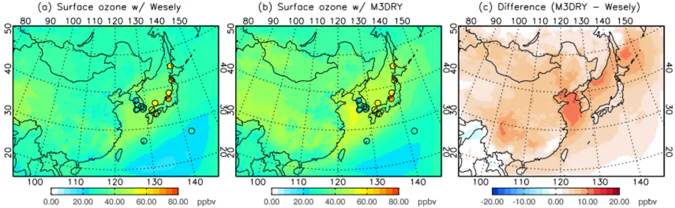
Figure 3.Monthly mean O3concentrations in surface air over East Asia for May 2004. The left and middle panels show results from the
WRF-Chem model using identical emissions and meteorological input data but different dry deposition schemes,(a)Wesely and(b)M3DRY. Observations from the NIER and EANET sites are denoted with colored closed circles. The O3concentration differences between the two simulations are shown in the right panel(c).
better resolved in the Wesely than in the M3DRY. Moreover, the underestimates of daytime values are consistently shown in the two different M3DRY applications: standalone and on-line. In fact, the online approach that uses the stomata resis-tance directly from the land surface model performs slightly better than the standalone M3DRY for reproducing the day-time values. Understanding this discrepancy is also important but beyond the scope of our present work. We plan to exam-ine this issue in the future study.
The largest discrepancy between the Wesely and the obser-vation occurs at the Mae Moh site, where the model cannot capture the peak in the morning and overestimates the ob-served values at night. As discussed above, the Mae Moh site is located in the tropical forest (Matsuda et al., 2005), but the model grid corresponding to the Mae Moh site is assigned as a cropland/pasture. We believe that the model horizontal resolution is too coarse to properly represent the observation site in northern Thailand and is likely the cause for the dis-crepancy between the model and the observations.
Nevertheless, we find that the Wesely successfully repro-duces the observed diurnal variation and the daytime values and performs better than the M3DRY particularly at the two US sites. We acknowledge that our evaluation is still too lim-ited to be applied for East Asia. However, the Manitou for-est observatory is a ponderosa pine plantation in the middle of shrub land (Kim et al., 2010), which is prevalent in East Asia, especially in the middle of China (Fig. 5a). Therefore, our evaluation provides limited but valid guidance of how the two dry deposition schemes perform over the majority of the East Asian land. We emphasize here that our evaluation does not represent East Asia in its entirety, and in situ ozone dry deposition velocity measurements thus are critical and necessary for enhancing our understanding of ozone loss and modeling capability for East Asia.
Figure 4.Hourly mean O3 concentrations averaged over(a)the NIER sites (left) and(b)EANET sites (right) for May 2004. The simulated values were sampled from the model grids that corre-spond to the site locations. The observations are denoted with open circles, and the simulated values with the Wesely and the M3DRY are shown using plus signs and triangles, respectively.
4 Simulated ozone concentrations in East Asia
Figure 3 shows the observed and simulated monthly mean ozone concentrations in surface air over East Asia for May 2004. The observations show a spatial gradient in which the values at polluted urban sites in Korea are lower than those at clean rural sites in Japan. Ozone losses by the titration of high NO in large megacities explain this observed spatial pattern with low values in Korea.
The simulated ozone concentrations with the two schemes also show a similar spatial gradient, which is high over the downwind ocean and relatively low over the continent. The model generally captures the observed spatial pattern, but the simulated pattern is not as clear as the observation because the model spatial resolution is not fine enough to capture concentrated pollution plumes at urban sites in Korea and to delineate sharp coastline variation in Japan.
Table 3.Surface ozone concentration (ppbv) and ozone dry deposi-tion velocity (m s−1, value in parentheses) in May and June 2004.
Wesely M3DRY
May 31.4 (0.24) 36.1 (0.10) June 32.2 (0.24) 36.1 (0.12)
schemes such that the Wesely values are significantly lower than those of the M3DRY. The simulated ozone difference between the two schemes is up to 10 ppbv for the monthly mean and is 4.7 ppbv for the domain mean (Table 3). The largest differences occur in the Yellow Sea and northwestern Pacific. We find that the simulated ozone differences are spa-tially inconsistent with the differences of the simulated dry deposition velocities between the two schemes. As shown in Fig. 1, the largest difference of the simulated dry deposition velocity appears on the continents, but the ozone concentra-tions difference is the greatest over the downwind ocean. We think that this feature is caused by the efficient ozone export from the polluted continent to the downwind oceans, where ozone accumulates (Goldberg et al., 2014). In addition, the ozone differences over the ocean may significantly be at-tributed to excessively high surface water resistance (low de-position loss) in the M3DRY relative to the Wesely. This is-sue is further discussed in Sect. 5. The export of ozone pre-cursors also contributes to high ozone over the oceans, but is relatively minor compared with the direct ozone export.
Table 3 summarizes the simulated surface ozone concen-tration and ozone dry deposition velocity averaged over the domain for May and June 2004, respectively, to examine their seasonal variation from spring to summer. We do not find considerable change in the simulated values between the 2 months except that the ozone dry deposition velocity with the M3DRY slightly increases in June relative to May be-cause of the increase of the vegetation cover. However, the ozone concentration remains the same in June compared with May because an increased ozone production offsets the in-creased ozone loss through dry deposition.
Figure 4 shows the hourly mean observed and simulated ozone concentrations averaged at the NIER sites in Korea and EANET sites in Japan for May 2004. The simulated values are sampled from the corresponding model grids to the observation sites for this comparison. The diurnal varia-tion differs between the two networks such that the observed ozone concentrations in Korea show a strong diurnal varia-tion, a peak in the afternoon and a minimum at night, which reflects a direct influence from local pollution.
The model generally captures the observed diurnal vari-ation, but also shows considerable discrepancies from the observations (Fig. 4). For example, at the NIER sites in Korea, the M3DRY overestimates the observations by 4.4– 17.1 ppbv. This high bias is reduced when we use the Wesely although the model still cannot capture the lowest ozone
con-Figure 5.Land-use data from the USGS (left) and MODIS data sets (right). The color-coding scheme used to denote the different sur-face types is consistent for the data sets and follow the USGS data set coloring (Table 4). We used the mapping information (Table 5) to illustrate the MODIS data.
centration in the early morning, caused by the NO titration during the rush hour traffic. We further examine this issue in Sect. 5.
On the other hand, the simulated ozone concentrations are lower than the observations at the EANET sites. This low bias is consistently shown in the model with both the We-sely and the M3DRY. The ozone differences between the two methods are 4.6–5.1 ppbv, smaller than 5.4–7.4 ppbv at the NIER sites. Although the M3DRY shows smaller biases than the Wesely, it is difficult to validate the dry deposition simu-lation alone because the EANET sites are primarily located at the coast, where the ocean heavily influences the observed ozone concentrations. It is known that the model and obser-vation discrepancies at the coastal sites are caused by the model’s inability to simulate steep sub-grid land-to-sea gra-dients at a mixing depth (Gao and Wesely, 1994; Loughner et al., 2011) that is shallower over the ocean compared with the continent. Our model with 45×45 km spatial resolution
may not adequately represent the shallow mixing depth at the EANET sites.
Although the model reproduces the certain observed fea-tures as shown in the comparisons in Figs. 3 and 4, it is dif-ficult to determine the scheme with the best performance for the observed ozone concentrations in East Asia. However, as discussed in Sect. 3, the model with the Wesely repro-duced the observed dry deposition velocities better than the M3DRY. Therefore, we use the Wesely results for our subse-quent analysis below, where we examine the simulated sen-sitivity to other input parameters.
5 Effect of surface-type uncertainty on ozone concentrations
Table 4.USGS 24 land-use data categories.
Land use Land use category description
1 Urban and built-up land 2 Dryland cropland and pasture 3 Irrigated cropland and pasture
4 Mixed dryland/irrigated cropland and pasture 5 Cropland/grassland mosaic
6 Cropland/woodland mosaic 7 Grassland
8 Shrubland
9 Mixed shrubland/grassland 10 Savanna
11 Deciduous broadleaf forest 12 Deciduous needleleaf forest 13 Evergreen broadleaf 14 Evergreen needleleaf 15 Mixed forest 16 Water bodies 17 Herbaceous wetland 18 Wooden wetland
19 Barren or sparsely vegetated 20 Herbaceous tundra
21 Wooded tundra 22 Mixed tundra 23 Bare ground tundra 24 Snow or ice
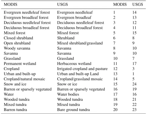
as a default option (Table 4). Here we explore the model sen-sitivity to the land-use data using the USGS and the MODIS land-use data (Friedl et al., 2002), which are widely used in meteorological research. In order to use the MODIS data, we developed a mapping table between the two data sets (Ta-ble 5), which was used to implement the MODIS land-use data in the WRF-Chem simulations below.
Figure 5 shows the USGS and the MODIS land-use data. In general, vegetation types identified by the two data sets are generally consistent for East Asia, but we find certain ences as well, especially for south China. One notable differ-ence is that the USGS classifies the Korean peninsula as sa-vanna, which differs from the MODIS classification (mixed forest). The different surface-type classifications affect ozone dry deposition calculations in the model as discussed below. Figure 6 shows the differences of dry deposition velocities and ozone concentrations in the model using the two land-use data sets: MODIS and USGS. Here we land-use the Wesely of which the simulated dry deposition velocities were consis-tent with the observations and were more sensitive to surface types than the M3DRY. The simulated differences of the dry deposition velocities reflect the different surface-type classi-fications between the two data sets. We find lower dry depo-sition velocities for East Asia using the MODIS compared with values with the USGS. The largest discrepancy occurs in southern China, where the surface type was changed from
Figure 6.Differences in dry deposition velocity (left) and monthly
mean O3 concentration in the surface air (right) between the
MODIS and USGS land-use data using the Wesely scheme for May 2004.
cropland/pasture, cropland/grassland mosaic, shrubland, and savanna to mixed forest (Fig. 5). This surface-type change increased the surface resistances and thus decreased the dry deposition velocity. On the other hand, the calculations in Manchuria and Republic of the Union of Myanmar showed increased dry deposition velocities because the surface types there were changed from mixed forest to cropland/pasture or evergreen broadleaf.
The change of the land-use data from the USGS to the MODIS results in an increase of the monthly mean ozone concentration by 10.2 ppbv in southern China and the down-wind regions, including Korea, Japan and the north Pacific for May. The average ozone concentration over the domain is increased with the MODIS land-use data by 1.3 % compared with the USGS data. This change seems negligible, but in the urban and industrialized regions the ozone increase with the MODIS data is much greater by 5.1 ppbv (13 %) compared with the USGS data, indicating the considerable sensitivity of ozone simulations to the surface-type classification.
The simulated sensitivity is also shown in the comparison of the hourly mean ozone concentrations at the NIER sites in Korea (Fig. 7). We find an increase of ozone concentra-tions averaged at all the sites by 3.9 ppbv simply by chang-ing the surface type from savanna to mixed forest, urban and built-up land. The model with the MODIS performs slightly worse than that with the USGS, but the model spatial reso-lution was still too coarse to represent surface-type inhomo-geneity at the sites in Korea, which are primarily in urban regions. The surface-type sub-grid scale variability may also be a potentially important source for model uncertainty. On the other hand, the model shows minimal changes in ozone at the EANET sites located near the sea.
Table 5.Land-use mapping between the 20-category International Geosphere-Biosphere Programme (IGBP)-Modified MODIS and 24-category USGS schemes.
MODIS USGS MODIS USGS
Evergreen needleleaf forest Evergreen needleleaf 1 14 Evergreen broadleaf forest Evergreen broadleaf 2 13 Deciduous needleleaf forest Deciduous needleleaf forest 3 12 Deciduous broadleaf forest Deciduous broadleaf forest 4 11 Mixed forest Mixed forest 5 15 Closed shrubland Shrubland 6 8 Open shrubland Mixed shrubland/grassland 7 9 Woody savanna Savanna 8 10
Savanna Savanna 9 10
Grassland Grassland 10 7 Permanent wetland Herbaceous wetland 11 17 Cropland Irrigated cropland and pasture 12 3 Urban and built-up Urban and built-up Land 13 1 Cropland/natural mosaic Cropland/grassland mosaic 14 5 Snow and ice Snow or ice 15 24 Barren or sparsely vegetated Barren or sparsely vegetated 16 19 Water Water bodies 17 16 Wooded tundra Wooded tundra 18 21 Mixed tundra Mixed tundra 19 22 Barren tundra Bare ground tundra 20 23
Figure 7.Same as in Fig. 4 but the simulated O3concentrations were generated using the USGS (pluses) and MODIS land-use data (diamonds) with the Wesely scheme.
differences of the ozone dry deposition velocities and ozone concentrations. The dry deposition velocity largely increases up to 0.043 cm s−1and causes an ozone decrease as low as 8.7 ppbv over the ocean. This change explains 76 % of the previous overall ozone concentration difference between the two schemes over the ocean. Although the ozone dry deposi-tion loss is lower over the ocean compared with the continent, this result indicates that the model is highly sensitive to the water surface resistance, which has an important implication for estimating long-range ozone transport from a source to a downwind region.
Finally, we conduct a nested model simulation using a finer spatial resolution (15 km) focusing on the Korean peninsula to examine the effect of NOx titration on ozone
concentrations in polluted urban cities. Figure 9 compares
Figure 8.Differences in monthly mean O3dry deposition
veloci-ties (left) and monthly mean O3concentrations in surface air (right) between the default and sensitivity simulations. The sensitivity sim-ulation was conducted using the Wesely scheme and replacing the ocean surface resistance with the values from the M3DRY scheme for May 2004.
the simulated ozone concentrations from the nested model with the observations at the NIER sites in Korea. With the finer spatial resolution, the nested model yields lower ozone concentrations by the enhanced NOx titration because the
Figure 9.Hourly mean O3concentrations averaged over the NIER sites (left) for May 2004. The pluses and squares indicate results from the default (45×45 km) and nested models (15×15 km), re-spectively. The observations are denoted with the open circles. The differences between the two models are shown in the right panel.
6 Conclusions
We used the WRF-Chem model with the two widely used dry deposition schemes (Wesely and M3DRY) to evaluate the dry deposition simulations and to examine the sensitivity of the simulated surface air ozone concentrations to dry deposition calculations for East Asia. We found significant differences in ozone concentrations up to 10 ppbv for the monthly mean, primarily driven by the dry deposition velocity differences between the two schemes. The Wesely generates two-fold greater dry deposition velocity compared with the M3DRY under identical meteorological conditions because of the dis-crepancies in the surface resistance parameterization.
We compared the simulated dry deposition velocities with the observations from the BEACHON-ROCS campaign and the Niwot Ridge Ameriflux sites in the US and from the Mae Moh site in northern Thailand. The Wesely generally com-puted dry deposition velocities higher than the M3DRY and successfully reproduced the observed diurnal variation. The Wesely also reproduced the observed ozone concentrations at the polluted urban sites in Korea, but failed to capture the ob-servations at the clean sites in Japan, indicating the existence of other important factors for background ozone simulations in East Asia.
We conducted several sensitivity simulations using the different land-use data sets, water surface resistances, and model spatial resolutions to examine the uncertainty of ozone simulations for East Asia. The model results showed consid-erable changes in the simulated ozone concentrations, which suggested that the model was highly sensitive to such input data and the model resolution. The need for in situ observa-tions is high to constrain the dry deposition parameterization and its input data to improve the use of air quality models for East Asia.
The roles of vegetation have primarily been discussed for emissions of reactive biogenic volatile organic compounds (BVOCs) and for tropospheric photochemistry that enhances ozone production in East Asia (Kim et al., 2013; Bao et al.,
2010; Ran et al., 2011; Tie et al., 2013). The comprehen-sive evaluation of dry deposition schemes herein clearly indi-cates that deposition is also a critical physical process, which must be precisely constrained in regional and global air qual-ity assessments because ozone has tremendous implications for public health (Levy et al., 2001) and climate change. In addition, a number of experimental studies have clearly sug-gested that a substantial level of unknown/unobserved reac-tive BVOCs may enhance non-stomatal ozone dry deposi-tion rates (Kurpius and Goldstein, 2003; Hogg et al., 2007), which should be further examined using an improved model-ing and extensive observations.
Acknowledgements. This study was supported by the Korea Meteorological Administration Research and Development Program under the Grant CATER 2012-6121 and the National Research Foundation of Korea (NRF) grant funded by the Korean government (MISP) (2009-83527). The National Center for Atmospheric Research is operated by the University Corporation for Atmospheric Research under sponsorship from the National Science Foundation. Any opinions, findings and conclusions or recommendations expressed in this publication are those of the authors and do not necessarily reflect the views of the National Science Foundation.
Edited by: C. H. Song
References
Appel, K. W., Gilliland, A. B., Sarwar, G., and Gilliam, R. C.: Eval-uation of the Community Multiscale Air Quality (CMAQ) model version 4.5: Sensitivities impacting model performance: Part I – Ozone, Atmos. Environ., 41, 9603–9615, 2007.
Bao, H., Shrestha, K. L., Kondo, A., Kaga, A., and Inoue, Y.: Mod-eling the influence of biogenic volatile organic compound emis-sions on ozone concentration during summer season in the Kinki region of Japan, Atmos. Environ., 44, 421–431, 2010.
Businger, J. A., Wyngaard, J. C., Izumi, I., and Bradley, E. F.: Flux-profile relationships in the atmospheric surface layer, J. Atmos. Sci., 28, 181–189, 1971.
Byun, D. W. and Ching, J. K. S.: Science algorithms of the EPA Models3 Community Multiscale Air Quality (CMAQ) Modeling System, U.S. EPA, USA, 1999.
Chapman, E. G., Gustafson Jr., W. I., Easter, R. C., Barnard, J. C., Ghan, S. J., Pekour, M. S., and Fast, J. D.: Coupling aerosol-cloud-radiative processes in the WRF-Chem model: Investigat-ing the radiative impact of elevated point sources, Atmos. Chem. Phys., 9, 945–964, doi:10.5194/acp-9-945-2009, 2009.
Charusombat, U., Niyogi, D., Kumar, A., Wang, X., Chen, F., Guen-ther, A., Turnipseed, A., and Alapaty, K.: Evaluating a New Deposition Velocity Module in the Noah Land-Surface Model, Bound.-Lay. Meteorol., 137, 271–290, 2010.
Erisman, J. W., Vanpul, A., and Wyers, P.: Parametrization of surface-resistance for the quantification of atmospheric deposi-tion of acidifying pollutants and ozone, Atmos. Environ., 28, 2595–2607, 1994.
Friedl, M. A., McIver, D. K., Hodges, J. C. F., Zhang, X. Y., Mu-choney, D., Strahler, A. H., Woodcock, C. E., Gopal, S., Schnei-der, A., Cooper, A., Baccini, A., Gao, F., and Schaaf, C.: Global land cover mapping from MODIS: algorithms and early results, Remote Sens. Environ., 83, 287–302, 2002.
Gao, W. and Wesely, M. L.: Numerical modeling of the turbu-lent fluxes of chemically reactive trace gases in the atmospheric boundary-layer, J. Appl. Meteorol., 33, 835–847, 1994. Garratt, J. R.: The atmospheric boundary layer, Cambridge
univer-sity press, New York, USA, 85–114, 1994.
Gerosa, G., Derghi, F., and Cieslik, S.: Comparison of different al-gorithms for stomatal ozone flux determination from microme-teorological measurements, Water Air Soil Poll., 179, 309–321, 2007.
Goldberg, D. L., Loughner, C. P., Tzortziou, M., Stehr, J. W., Pick-ering, K. E., Marufu, L. T., and Dickerson, R. R.: Higher surface ozone concentrations over the Chesapeake Bay than over the ad-jacent land: Observations and models from the DISCOVER-AQ and CBODAQ campaigns, Atmos. Environ., 84, 9–19, 2014. Grell, G. A., Peckham, S. E., Schmitz, R., McKeen, S. A., Frost, G.,
Skamarock, W. C., and Eder, B.: Fully coupled “online” chem-istry within the WRF model, Atmos. Environ., 39, 6957–6975, 2005.
Hogg, A., Uddling, J., Ellsworth, D., Carroll, M. A., Pressley, S., Lamb, B., and Vogel, C.: Stomatal and non-stomatal fluxes of ozone to a northern mixed hardwood forest, Tellus B, 59, 514– 525, 2007.
Hong, S.-Y., Noh, Y., and Dudhia, J.: A New Vertical Diffusion Package with an Explicit Treatment of Entrainment Processes, Mon. Weather Rev., 134, 2318–2341, 2006.
Jacob, D. J., Crawford, J. H., Kleb, M. M., Connors, V. S., Bendura, R. J., Raper, J. L., Sachse, G. W., Gille, J. C., Emmons, L., and Heald, C. L.: Transport and Chemical Evolution over the Pacific (TRACE-P) aircraft mission: Design, execution, and first results, J. Geophys. Res., 108, 9000, doi:10.1029/2002JD003276, 2003. Jeong, J. I., Park, R. J., Woo, J. H., Han, Y. J., and Yi, S. M.: Source contributions to carbonaceous aerosol concentrations in Korea, Atmos. Environ., 45, 1116–1125, 2011.
Kim, S., Karl, T., Guenther, A., Tyndall, G., Orlando, J., Harley, P., Rasmussen, R., and Apel, E.: Emissions and ambient distri-butions of Biogenic Volatile Organic Compounds (BVOC) in a ponderosa pine ecosystem: interpretation of PTR-MS mass spec-tra, Atmos. Chem. Phys., 10, 1759–1771, doi:10.5194/acp-10-1759-2010, 2010.
Kim, S., Lee, M., Kim, S., Choi, S., Seok, S., and Kim, S.: Pho-tochemical characteristics of high and low ozone episodes ob-served in the Taehwa Forest observatory (TFO) in June 2011 near Seoul South Korea, Asia-Pac, J. Atmos. Sci., 49, 325–331, 2013. Ku, B. and Park, R. J.: Inverse modeling analysis of soil dust sources
over East Asia, Atmos. Environ., 45, 5903–5912, 2011. Kurpius, M. R. and Goldstein, A. H.: Gas-phase chemistry
domi-nates O3loss to a forest, implying a source of aerosols and
hy-droxyl radicals to the atmosphere, Geophys. Res. Lett., 30, 1371, doi:10.1029/2002GL016785, 2003.
Lelieveld, J. and Dentener, F. J.: What controls tropospheric ozone?, J. Geophys. Res., 105, 3531–3551, 2000.
Levy, J. I., Carrothers, T. J., Tuomisto, J. T., Hammitt, J. K., and Evans, J. S.: Assessing the public health benefits of reduced ozone concentrations, Environ. Health Persp., 109, 1215–1226, 2001.
Li, J., Wang, Z. F., Akimoto, H., Gao, C., Pochanart, P., and Wang, X. Q.: Modeling study of ozone seasonal cycle in lower troposphere over east Asia, J. Geophys. Res., 112, D22S25, doi:10.1029/2006JD008209, 2007.
Loughner, C. P., Allen, D. J., Pickering, K. E., Zhang, D. L., Shou, Y. X., and Dickerson, R. R.: Impact of fair-weather cumulus clouds and the Chesapeake Bay breeze on pollutant transport and transformation, Atmos. Environ., 45, 4060–4072, 2011. Lovett, G. M. and Reiners, W. A.: Canopy structure and cloud
wa-ter deposition in subalpine coniferous forests, Tellus B, 38, 319– 327, 1986.
Matsuda, K., Watanabe, I., and Wingpud, V.: Ozone dry deposition above a tropical forest in the dry season in northern Thailand, Atmos. Environ., 39, 2571–2577, 2005.
Matsuda, K., Watanabe, I., Wingpud, V., Theramongkol, P., and Ohizumi, T.: Deposition velocity of O3and SO2in the dry and
wet season above a tropical forest in northern Thailand, Atmos. Environ., 40, 7557–7564, 2006.
National Centers for Environmental Prediction, N.W.S.N.U.S.D.o.C.: NCEP FNL Operational Model Global Tropospheric Analyses, continuing from July 1999, Research Data Archive at the National Center for Atmospheric Research, Computational and Information Systems Laboratory, Boulder, CO, 2000
Noilhan, J. and Planton, S.: A Simple Parameterization of Land Sur-face Processes for Meteorological Models, Mon. Weather Rev., 117, 536–549, 1989.
Ohara, T., Akimoto, H., Kurokawa, J., Horii, N., Yamaji, K., Yan, X., and Hayasaka, T.: An Asian emission inventory of an-thropogenic emission sources for the period 1980–2020, At-mos. Chem. Phys., 7, 4419–4444, doi:10.5194/acp-7-4419-2007, 2007.
Otte, T. L. and Pleim, J. E.: The Meteorology-Chemistry Inter-face Processor (MCIP) for the CMAQ modeling system: up-dates through MCIPv3.4.1, Geosci. Model Dev., 3, 243–256, doi:10.5194/gmd-3-243-2010, 2010.
Park, R. J. and Kim, S. W.: Air quality modeling in East Asia: present issues and future directions, Asia-Pac. J. Atmos. Sci., 50, 105–120, 2014.
Perrier, A.: Land surface processes: vegetation, in: Land surface processes in atmospheric general circulation models, Cambridge university press, New York, USA, 395–448, 1982.
Pleim, J. E., Xiu, A., Finkelstein, P. L., and Otte, T. L.: A Cou-pled Land-Surface and Dry Deposition Model and Comparison to Field Measurements of Surface Heat, Moisture, and Ozone Fluxes, Water Air Soil Poll., 1, 243–252, 2001.
Ran, L., Zhao, C. S., Xu, W. Y., Lu, X. Q., Han, M., Lin, W. L., Yan, P., Xu, X. B., Deng, Z. Z., Ma, N., Liu, P. F., Yu, J., Liang, W. D., and Chen, L. L.: VOC reactivity and its effect on ozone production during the HaChi summer campaign, Atmos. Chem. Phys., 11, 4657–4667, doi:10.5194/acp-11-4657-2011, 2011. Rannik, Ü., Altimir, N., Mammarella, I., Bäck, J., Rinne, J.,
deposition into a boreal forest over a decade of observa-tions: evaluating deposition partitioning and driving variables, Atmos. Chem. Phys., 12, 12165–12182, doi:10.5194/acp-12-12165-2012, 2012.
Tie, X., Geng, F., Guenther, A., Cao, J., Greenberg, J., Zhang, R., Apel, E., Li, G., Weinheimer, A., Chen, J., and Cai, C.: Megac-ity impacts on regional ozone formation: observations and WRF-Chem modeling for the MIRAGE-Shanghai field campaign, At-mos. Chem. Phys., 13, 5655–5669, doi:10.5194/acp-13-5655-2013, 2013.
Tsai, J. L., Chen, C. L., Tsuang, B. J., Kuo, P. H., Tseng, K. H., Hsu, T. F., Sheu, B. H., Liu, C. P., and Hsueh, M. T.: Observation of SO2dry deposition velocity at a high elevation flux tower over an
evergreen broadleaf forest in Central Taiwan, Atmos. Environ., 44, 1011–1019, 2010.
Turnipseed, A. A., Burns, S. P., Moore, D. J. P., Hu, J., Guenther, A. B., and Monson, R. K.: Controls over ozone deposition to a high elevation subalpine forest, Agr. Forest Meteorol., 149, 1447–1459, 2009.
Wesely, M. L.: Parameterization of surface resistances to gaseous dry deposition in regional-scale numerical models, Atmos. Envi-ron., 23, 1293–1304, 1989.
Woo, J. H., Choi, K. C., Kim, H. K., Baek, B. H., Jang, M., Eum, J. H., Song, C. H., Ma, Y. I., Sunwoo, Y., Chang, L. S., and Yoo, S. H.: Development of an anthropogenic emissions processing system for Asia using SMOKE, Atmos. Environ., 58, 5–13, 2012. Wu, S., Mickley, L. J., Jacob, D. J., Logan, J. A., Yantosca, R. M., and Rind, D.: Why are there large differences between models in global budgets of tropospheric ozone?, J. Geophys. Res., 112, D05302, doi:10.1029/2006JD007801, 2007.
Wu, Z., Wang, X., Chen, F., Turnipseed, A. A., Guenther, A. B., Niyogi, D., Charusombat, U., Xia, B., William Munger, J., and Alapaty, K.: Evaluating the calculated dry deposition veloci-ties of reactive nitrogen oxides and ozone from two community models over a temperate deciduous forest, Atmos. Environ., 45, 2663–2674, 2011.