www.biogeosciences.net/8/715/2011/ doi:10.5194/bg-8-715-2011
© Author(s) 2011. CC Attribution 3.0 License.
Biogeosciences
Age structure and disturbance legacy of North American forests
Y. Pan1, J. M. Chen2, R. Birdsey1, K. McCullough1, L. He2, and F. Deng2
1US Forest Service Northern Global Change Program, Newtown Square, PA 19073, USA 2Department of Geography University of Toronto, Ontario, M5S 3G3, Canada
Received: 17 December 2009 – Published in Biogeosciences Discuss.: 10 February 2010 Revised: 15 February 2011 – Accepted: 16 February 2011 – Published: 18 March 2011
Abstract. Most forests of the world are recovering from a past disturbance. It is well known that forest disturbances profoundly affect carbon stocks and fluxes in forest ecosys-tems, yet it has been a great challenge to assess disturbance impacts in estimates of forest carbon budgets. Net sequestra-tion or loss of CO2by forests after disturbance follows a
pdictable pattern with forest recovery. Forest age, which is re-lated to time since disturbance, is a useful surrogate variable for analyses of the impact of disturbance on forest carbon. In this study, we compiled the first continental forest age map of North America by combining forest inventory data, historical fire data, optical satellite data and the dataset from NASA’s Landsat Ecosystem Disturbance Adaptive Processing Sys-tem (LEDAPS) project. A companion map of the standard deviations for age estimates was developed for quantifying uncertainty. We discuss the significance of the disturbance legacy from the past, as represented by current forest age structure in different regions of the US and Canada, by ana-lyzing the causes of disturbances from land management and nature over centuries and at various scales. We also show how such information can be used with inventory data for analyzing carbon management opportunities. By combin-ing geographic information about forest age with estimated C dynamics by forest type, it is possible to conduct a sim-ple but powerful analysis of the net CO2uptake by forests,
and the potential for increasing (or decreasing) this rate as a result of direct human intervention in the disturbance/age sta-tus. Finally, we describe how the forest age data can be used in large-scale carbon modeling, both for land-based biogeo-chemistry models and atmosphere-based inversion models, in order to improve the spatial accuracy of carbon cycle sim-ulations.
Correspondence to: Y. Pan
1 Introduction
Most forests of the world are recovering from a past distur-bance. According to a recent global forest resources assess-ment, 36% of the world’s 4 billion ha of forest are classi-fied as primary forest, i.e., showing no significant human im-pact (FAO, 2005). The same report estimates that 104 mil-lion ha yr−1of the world’s forests, or 3% of the total area, are
disturbed each year by fire, pests, and weather, though this is a significant underestimate of the disturbance rate because of incomplete reporting by countries. For the US, it is esti-mated that about half of the forest area, or 152 million ha, is disturbed each decade, but this estimate covers a wide range of disturbance types including timber harvesting and graz-ing which affect more area than natural disturbances (Bird-sey and Lewis, 2003). In Canada, wildfires were the largest disturbance type in the 20th century, affecting an average of 2.6 million ha per year in the last two decades (Stocks et al., 2002; Weber and Flannigan, 1997). Insect pests are also significant and likely to increase in the future according to model simulations (Kurz et al., 2008a).
The net sequestration or loss of CO2by forests after
distur-bance follows a predictable pattern determined by age, site, climate, and other factors (Pregitzer and Euskirchen, 2004). Typically, regenerating forests grow at an accelerating rate that reaches a peak at about the time the canopy closes, fol-lowed by a declining rate of increase that may last for cen-turies. A recent review of data from old-growth forests con-cluded that they may continue to sequester atmospheric CO2
forest floor, causing these pools to shift between sources and sinks over time.
In this paper we present a forest age map of the US and Canada, describe our approaches to develop this map and a companion map of standard deviation for age estimates that can be used for evaluating uncertainty. We discuss how such a map may be used with inventory data for analyzing carbon management opportunities and for other modeling applica-tions. Forest age, implicitly reflecting the past disturbance legacy, is a simple and direct surrogate for the time since disturbance and may be used in various forest carbon anal-yses that concern the impact of disturbances. By combin-ing geographic information about forest age with estimated C dynamics by forest type, it is possible to conduct a sim-ple but powerful analysis of the net CO2uptake by forests,
and the potential for increasing (or decreasing) this rate as a result of direct human intervention in the disturbance/age status. The biological potential of afforestation, reforesta-tion, and forest management to offset fossil fuel emissions may be estimated with knowledge of the area available for the activity and estimated changes in ecosystem C by age. This kind of analysis is regionally and globally significant with respect to managing the carbon cycle. According to the latest IPCC report, the potential of global forestry mit-igation measures may be as high as 13.8 Pg CO2yr−1at
car-bon prices of $100 t−1CO2(Nabuurs et al., 2007). We also
briefly described how such information can be applied in large-scale carbon modeling, using both land-based biogeo-chemistry models and atmosphere-based inversion models for improving the accuracy of simulated carbon dynamics.
2 Data and methods
To generate the age map, we integrated remote sensing data with the age information from forest inventories, disturbance datasets, and land-use/land cover change data. Because Canada and the US have different systems and approaches to collect and manage forest and land data, different approaches were used to produce spatial forest age information for these two countries (Table 1).
2.1 Approach for Canada
2.1.1 Inventory and disturbance data
In Canada, the national forest inventory (CanFI) is compiled about every five years by aggregating provin-cial and territorial forest management inventories (www.nrcan-rncan.gc.ca). Stand-level data provided by the provincial and territorial management agencies are converted to a national classification scheme and then ag-gregated to ecological and political classifications. The data used for this study were derived from the dataset developed by Penner et al. (1997), which was the gridded data at 10 km resolution and originally compiled from Canada’s
Forest Inventory (CanFI) 1991 (1994 version) (Lowe et al., 1996). The data also include the forested area-fractions of age classes (0–20, 21–40, 41–60, 61–80, 81–100, 101–120, 121–140, 141–160 and older). Since the inventory data was outdated, we used more recent remote sensing data to update the age information (only about 55% of the total forest area of Canada is inventoried; unmanaged lands are not inventoried).
Historical fire data, based on the Canadian Large-Fire Data Base (LFDB), were compiled from datasets maintained by provincial, territorial and federal agencies (Amiro et al., 2001). The dataset provides polygons mapped in a Geo-graphical Information System (GIS), which delineates the outlines of fires and associated attribute information, such as fire start date, year of fire, fire number, and final area burned. The dataset includes 8,880 polygons of fire scars larger than 200 ha distributed across much of the boreal and taiga eco-zones, going back as far as 1945 in some areas (Stocks et al., 2003). The LFDB includes fire records generally for 1959– 1995.
2.1.2 Remote sensing and age distribution
Satellite imagery was used to supplement data from inven-tory and LFDB to complete a Canada-wide forest stand age map in 2003. The data from the VEGETATION sensor on-board the SPOT4 satellite were used in this study. The angu-lar normalization scheme developed for AVHRR (Chen and Cihlar, 1997) was applied to VEGETATION 10-day cloud-free synthesis data from June to August 1997. Ratios of shortwave infrared (SWIR) to NIR in these 9 images, named as the disturbance index (DI), were averaged for each pixel to produce a single ratio image for the mid-summer. The aver-aging process was necessary as SWIR signals are sensitive to rainfall events. Co-registered with LFDB data, the relation-ship between the mean SWIR/NIR ratio in the summer and the number of years since the last burn (Amiro and Chen, 2003) was used to develop an algorithm for dating/mapping fire scar areas. The dating algorithms have accuracy of±7 yr for scar ages smaller than 25 yr (Amiro and Chen, 2003). The satellite imagery from VEGETATION-SPOT were used to develop the fire scar maps of 25 yr from 1973–1997, in-cluding the fire scars that were not included in LFDB. The results show that the total disturbed area in any five-year pe-riod is within 10% variation of the total reported by Kurz and Apps (1995). The VEGETATION data were also used to ex-tend the fire record of LFDB from 1995 to 2003 by detecting burned areas annually.
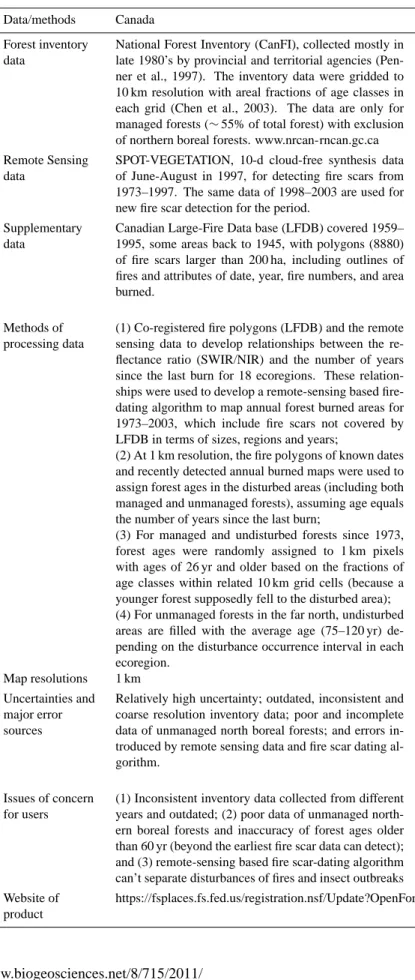
Table 1. Comparison of data and methods used to develop forest age maps for Canada and the US.
Data/methods Canada The US
Forest inventory data
National Forest Inventory (CanFI), collected mostly in late 1980’s by provincial and territorial agencies (Pen-ner et al., 1997). The inventory data were gridded to 10 km resolution with areal fractions of age classes in each grid (Chen et al., 2003). The data are only for managed forests (∼55% of total forest) with exclusion of northern boreal forests. www.nrcan-rncan.gc.ca
National Forest Inventory Analysis (FIA), collected pe-riodically (every 5–6 yr, currently annual), at∼150 000 sample locations. There are over 100 000 data points for this study. FIA data include stand age with mostly one condition (even or average age), or 2–3 conditions of multiple ages (uneven-aged). Alaska has incomplete data. www.fia.fs.fed.us
Remote Sensing data
SPOT-VEGETATION, 10-d cloud-free synthesis data of June-August in 1997, for detecting fire scars from 1973–1997. The same data of 1998–2003 are used for new fire scar detection for the period.
NASA Landsat Ecosystem Disturbance Adaptive Pro-cession System (LEDAPS). Disturbed areas between 1990 and 2000, 500 m pixels with fractions of disturbed areas summarized from mosaics at 28.5 m resolution. Supplementary
data
Canadian Large-Fire Data base (LFDB) covered 1959– 1995, some areas back to 1945, with polygons (8880) of fire scars larger than 200 ha, including outlines of fires and attributes of date, year, fire numbers, and area burned.
Monitoring Trend in Burn Severity (MTBS), with burn-ing severity values (1–4) and fire perimeters. Four states in the western US were selected for this study, which in-clude 1405 fire events in 1987–2001.
Areas of annual regenerations between 1990 and 2000 were compiled from FIA data
Methods of processing data
(1) Co-registered fire polygons (LFDB) and the remote sensing data to develop relationships between the re-flectance ratio (SWIR/NIR) and the number of years since the last burn for 18 ecoregions. These relation-ships were used to develop a remote-sensing based fire-dating algorithm to map annual forest burned areas for 1973–2003, which include fire scars not covered by LFDB in terms of sizes, regions and years;
(2) At 1 km resolution, the fire polygons of known dates and recently detected annual burned maps were used to assign forest ages in the disturbed areas (including both managed and unmanaged forests), assuming age equals the number of years since the last burn;
(3) For managed and undisturbed forests since 1973, forest ages were randomly assigned to 1 km pixels with ages of 26 yr and older based on the fractions of age classes within related 10 km grid cells (because a younger forest supposedly fell to the disturbed area); (4) For unmanaged forests in the far north, undisturbed areas are filled with the average age (75–120 yr) de-pending on the disturbance occurrence interval in each ecoregion.
(1) Developed age polygons based on FIA plot stand ages and assigned ages to 1 km (or 250 m) grid cells; (2) Used TM/ETM scenes from LEADAPS to de-velop reflectance ratios (SWIR/NIR), i.e. disturbance index (DI), for 1990 and 2000. DIs were normalized and the differences (NDDIs) were used for detecting disturbances and making a disturbance map, which was validated using MTBS data;
(3) The FIA data of forest regeneration areas were forced to establish the relationship with the disturbed ar-eas in each county; and used to find a threshold NDDI of for separating disturbances that occurred in 1991–1995 and 1996–2000;
(3) Converted the disturbance dating to an age map of young regeneration forests for age groups of 0–5 and 6–10 yr;
(4) Young forest ages were superimposed on top of the Voronoi data to replace values of grid cells in the FIA-based age map.
Map resolutions 1 km 1 km and 250 m
Uncertainties and major error sources
Relatively high uncertainty; outdated, inconsistent and coarse resolution inventory data; poor and incomplete data of unmanaged north boreal forests; and errors in-troduced by remote sensing data and fire scar dating al-gorithm.
Relatively low uncertainty; biases of FIA stand age samples; averaging ages of uneven-aged forests in de-veloping age polygons; inconsistency of acquisition dates from LEDAPS dataset for developing DIs for year 1990 and 2000; and errors from the algorithm dating by using FIA data to set the thresholds.
Issues of concern for users
(1) Inconsistent inventory data collected from different years and outdated; (2) poor data of unmanaged north-ern boreal forests and inaccuracy of forest ages older than 60 yr (beyond the earliest fire scar data can detect); and (3) remote-sensing based fire scar-dating algorithm can’t separate disturbances of fires and insect outbreaks
(1) Metadata approach, ages of uneven-aged forests were averaged; and (2) landscape disturbances that oc-curred before (or after) 1990s were not processed in this study and the effects could be missed in the age map if the inventory data did not cover the disturbed areas – this could be a particular problem for the western US. Website of
product
used to replace the age data in the gridded inventory data. Fire polygons in the LFDB provided data for the northern boreal regions (unmanaged forests without inventory data), but only included large fires over the period of 1945 to 1995 (for dating the forests that are about younger than 60 yr in 2003). Remote sensing imagery was further used to fill in the data gaps both in space and time. Annual forest burned area maps for years between 1973 and 2003 were constructed by the approaches described previously. However, the older age classes (>25 yr) in the inventory are unchanged because we assumed that the inventory age-class data were correct for all grid cells that were not disturbed after 1973. In the com-bination of these three types of data, a 10×10 km grid cell in the forest inventory was divided into 100 pixels at 1 km resolution. Pixels of different age classes were replaced by the fire polygons of known dates or by recent fire scars if detected by remote sensing. For the other undisturbed areas (not identified by fire scars and remote sensing) of the man-aged forests, pixels were randomly assigned with ages older than 26 yr, based on the area fractions in each age class re-ported in the inventories (after adjusted to the fractions of areas dated by remote sensing and fire scars). For the un-managed forests in the far north, the limited inventory data indicated that most of forests are less than 120 yr. Thus, pix-els were assigned with the average age (75–120 yr) depend-ing on the disturbance occurrence intervals in each ecoregion that were used to estimate an average life span of forests (be-cause forest ages younger than the age class of 61–80 yr are supposedly identified by fire scars and remote sensing, and there were no other disturbances such as harvesting occurred in unmanaged forests).
2.2 Approach for the US
2.2.1 FIA age information and disturbance data
Development of the age map for the US is based primar-ily on field sampling by the Forest Inventory and Analy-sis (FIA) Program, a continuous inventory and assessment of US forests (Bechtold and Patterson, 2005). This national in-ventory provides periodic estimates of area, timber volume, tree biomass, growth, mortality, and harvest of wood prod-ucts (Smith et al., 2001). The inventory also characterizes important forest attributes such as forest type, tree density, and stand age. Most forests of the US are sampled, except for some remote areas where only partial inventories have been conducted, most importantly Alaska. Alaska is currently be-ing inventoried and comparable data may be available within a decade. The FIA estimates are based on tree measurements from a very large statistical sample (more than 150 000 sam-ple locations), and mathematical models to estimate forest attributes such as biomass (Birdsey and Schreuder, 1992). Stand age is estimated at sample plots by examining tree rings from cores of selected trees. Determination of stand age can be an inexact process because only one or a few trees,
selected to represent the average age of the sample area, are cored. Over 100 000 data points were used in this study. We also compiled forest regeneration areas for 1990–2000 from FIA database for the age-dating purpose.
2.2.2 Remote sensing and age distribution
The NASA Landsat Ecosystem Disturbance Adaptive Pro-cessing System (LEDAPS) (Masek et al., 2008) applied re-mote sensing data, particularly Landsat TM/ETM data over the decades, to detect land disturbances and forest cover changes. LEDAPS produces disturbance maps at 28.5 m resolution for selected areas and at 500 m resolution for the whole of North America. It also provides the fraction of disturbed area within each 500 m pixel by summariz-ing the 28.5 m resolution information. In addition, the re-flectance data for North America at 500 m resolution were also available for this analysis. We used atmospherically corrected 500 m North America surface reflectance mosaics from LEDAPS (1990 and 2000) to extract the disturbance in-formation, through pair-wise comparison of reflectance data. The disturbance indices (DIs), the ratios of the shortwave in-frared (TM band 5) to near inin-frared (TM band 4) reflectance (Amiro and Chen, 1993), were developed for 1990 and 2000 and normalized. The DI is higher following disturbances, then decreases as vegetation density increases towards the pre-disturbed status. The differences of normalized DIs (ND-DIs) were used for detecting disturbances or forest regrowth (i.e. a positive value indicates disturbance), and making dis-turbance maps. The Monitoring Trends in Burning Sever-ity (MTBS) data (http://mtbs.gov/index.html) were used as a reference to assess the accuracy of forest disturbance maps (He et al., 2011). The MTBS is mapped at 30 m resolution using the differenced Normalized Burn Ratio (dNBR). The data from 4 states of the western US (California, Idaho, Ore-gon and Washington) were selected for accuracy assessment, composed of 1405 fire events (greater than 4 km2)for 1987– 2001.
The average stand ages of FIA plots were used to develop the age map using Voronoi polygons. Voronoi polygons show the entire area around a plot location that it is near-est to its location. These can be assumed to represent fornear-est stands and their respective ages around each FIA plot. This method works well in high data density areas where there is high spatial coverage of FIA plot locations (East Coast) and not as well when there is low spatial coverage of plot loca-tions (Oklahoma). The polygon data were assigned to grid cells at 1 km resolution and then adjusted to the 2003 USFS Forest Type map (Ruefenacht et al., 2008). The forest ages range broadly from young growth in the southeastern region (∼10 yr) to old growth in western coasts (∼900 yr).
Fig. 1. (a) Forest age distribution in North America (excluding Alaska and Mexico), which was developed by combining forest inventory data
(of US and Canada) with several remote sensing based disturbance data sources. (b) The standard deviations of forest ages that characterize uncertainty in the age map (a).
time, being higher for newly disturbed areas. Assuming for-est regrowth starts immediately after disturbance, we devel-oped an algorithm to force total regenerated forest areas of the FIA statistics to relate to the total disturbed areas within each county (He et al., 2011). The NDDI values of pixels in each county were sorted in descending order and a threshold NDDI was chosen based on the fractions of regenerated for-est areas in two five-year groups (i.e. 1990–1995 and 1996– 2000). The threshold NDDI was used to separate pixels of disturbed areas into two age groups of young forests (1–5, and 6–10 yr) (He et al., 2011). Finally, the young forest ages were used to overlay and modify the inventory-based forest ages to produce the age map.
2.3 Uncertainty and major error sources of the age map
For the forest age map (Fig. 1a), we also developed a stan-dard deviation (std) map (Fig. 1b) for quantifying uncer-tainty. The std map provides a useful uncertainty measure for users to apply the age map in their studies. Because the data sources of Canadian and the US components are differ-ent, the methods for calculating std are also different. For the US, with high quality and massive forest inventory data, we have developed the age map at 250 m resolution based on age polygons generated from plot data using the GIS ap-proach (Pan et al., 2010). The standard deviation for each 1-km grid cell is calculated based on 16 sub-pixels. The de-viation reflects the uncertainty of spatial heterogeneity in age distribution and the GIS approach for interpolating plot data.
High uncertainty occurs in the rocky mountain regions and the west coast because forest age cohorts of young and long-lived trees are mixed over the landscape. Most of the de-viations in the eastern US are around 10 yr, indicating more homogeneous and young forest age structures (Fig. 1b).
For the Canadian component of the age map, the std was estimated using a “moving window” approach for each cen-ter pixel with 8 neighboring pixels. The deviation reflects the spatial heterogeneity of age distribution but at a much coarser resolution than the US data, revealing uncertainty in those undisturbed forests where the age fractions from the inventory data map (10×10 km) were randomly assigned for down-scaled 1-km pixels. The least uncertainty is for those grid-cells where forest ages were identified by the fire scar data and remote sensing. The highest uncertainty happens to the undisturbed forest areas in British Columbia, where a large discrepancy in age cohorts between young and old growth and the random age assignment in down-scaled pix-els jointly cause the uncertainty to be around 50 yr (Fig. 1b). Less than 1% of grid-cells located in the west coast of the US and British Columbia have high deviations greater than 80 yr, resulting from great spatial diversity of age mosaics in a neighborhood consisting of both newly generated young forests and long-lived old growth (Fig. 1a).
of very recent disturbances (1990–2000). The Canadian map was based on older inventory data that was gridded at 10 km resolution and only covered managed forests (55% of total forests). However, historical fire polygon data (major dis-turbances for Canadian forests) over five decades provided valuable data, together with remote sensing, for detecting the perimeters and timing of disturbed forests. Thus, the major error sources or inaccuracy for the Canadian age map are from older, inconsistent, and coarse resolution inventory data, incomplete data of unmanaged northern boreal forests, and problems related to the poor spatial resolution of the in-ventory data (it was necessary to randomly assign ages to the down-scaled 1 km grid cells based on the inventoried frac-tions of age-classes in the 10 km grid cells because the exact location of each class within each grid cell is unknown). In addition, the remote sensing based approach also introduces errors in the algorithm dating (∼ ±7 yr) (Chen et al., 2003). For the US age map, errors could be derived from inaccurate determination of age at FIA sample plots, and from the use of average ages for uneven-aged stands when developing age polygons. For identifying the impact of recent disturbance on forest age pattern, the use of LEDAPS data included er-rors from inconsistency in acquisition dates for developing DIs for years from 1990 to 2000. Uncertainty can also be associated with a relatively arbitrary approach to algorithm dating by using the FIA data of forest regeneration to choose the spectral thresholds.
3 Age structure and disturbance legacy of North American forests
The forest age map (Fig. 1a) developed in this study shows the pattern of forest age structure in temperate and boreal ar-eas of North America. We regrouped age classes for mapping but the original age data for users preserve their variations (Table 1 includes the website address of the data). Although the approaches to develop forest age maps in Canada and the US are not exactly the same, the map results show consistent and smooth patterns across the boundaries between these two countries. Natural and human forces over the last two cen-turies together have shaped the age structure of forests in the US (Fig. 2) and Canada today (Birdsey et al., 2006; Kurz and Apps, 1999). Due to geographical features, land-use history, harvesting, and disturbance regimes, Canada in general has older forests than the US although there are some very old forests in the US. Pacific coast (∼900 yr) For example, 43% of forests in British Columbia are defined as old growth with ages between 120 and 200 yr, but there are large patches of younger forests (41%) in the early stages of recovery from wildfire and harvesting (BC Ministry of Forests, 2003). In contrast, forests in the Southeastern US have a distribution of younger age classes because of intensive management and harvesting for wood products. The regional histograms sum-marized from the areas of age-map pixels provide more
Drain on the Sawtimber Stand
1650 1700 1750 1800 1850 1900
Woo
d
Vo
lum
e (
millio
n
m
3 y
r
-1 )
0 50 100 150 200 250
Total Commodity Cut Fuelwood
Lumber Other
Wood Losses by Other Disturbances
Year
1650 1700 1750 1800 1850 1900
Wo
o
d
Vo
lum
e (
millio
n
m
3 y
r
-1 )
0 50 100 150 200 250
Total Other Losses Insects and Disease Farms Clearing Fires Waste
(a)
(b)
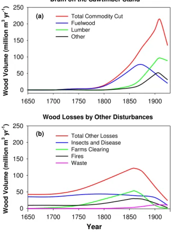
Fig. 2. Impacts of disturbances on forests in the past: (a) Drain on
the US Sawtimber Stand, 1650–1925 (unit: million cubic meters per year based on sawtimber volume); and (b) wood losses affected by other disturbances (based on the data from Birdsey et al., 2006).
tailed data of age structures and ranges in regions of the US and Canada (Figs. 3, 4 and 5). We illustrate how these re-gional forest age structures implicitly represent the land dis-turbance legacy from the past, and also relate the age patterns with land-use and disturbance history to contrast the past hu-man and natural causes.
3.1 The US Northeast, Northern Lakes and Northern Plains regions
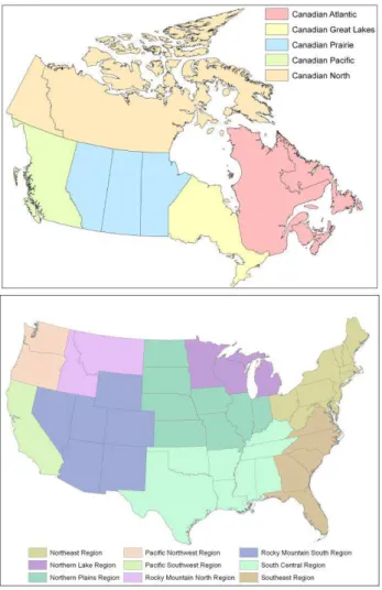
Fig. 3. Forest regions in Canada and the United States (Alaska is
not shown here).
more maple-beech-birch, oak-hickory, and oak-pine to more aspen-birch and spruce-fir because of climate factors. How-ever, roughly a decadal lag in shifting dominant forest age groups from the northeastern to the northern lakes and north-ern plains reflects the natural recovery of forests from west-ward agricultural clearing and abandonment and the pattern of forest harvest in the regions in the early 20th century (Fig. 4; Fedkiw, 1989; MacCleery, 1992). A lower represen-tation of the age groups older than 80 yr reflects the heavy harvest in the early 20th century (compared to the Canadian Atlantic Maritime region). Forests in these regions have po-tential to reach dominant ages of 100–120 yr old or more in next four to five decades. There are also indications of shift-ing species composition from white-red-jack pine types to deciduous Maple-beech-birch and oak-hickory types (Bird-sey and Lewis, 2003) as a result of natural succession. Lower representation of young forests is typical for middle-aged forests that are not mature enough to create gaps for the next wave of regeneration.
3.2 The US Southeast and South Central regions
Forests in the Southeast and South Central regions are domi-nated by young growth and have shorter average life-spans of approximately 80–100 yr, although some are as old as ∼180 yr (Fig. 4). Forests in the region are mostly composed of loblolly pine, slash pine, oak-pine, oak-hickory, oak-cum-cypress, and elm-ash-cottonwood, with slightly more de-ciduous types than coniferous types in the southeast region and much more deciduous types towards the south central region. In the first half of the 20th century much of the Southern forest was cutover and frequently burned (Larson 1960). Afterwards, large areas of the southeast and south central regions were converted to short-rotation pine planta-tions, mostly loblolly and shortleaf pines. These plantations are routinely harvested and replanted, which results in rel-atively evenly-distributed age groups less than 60 yr old for more than 80% of the forested area (Fig. 1a). Few stands reach more than 80 yr old (Fig. 4). Areas that are not in plan-tation forestry are still harvested frequently; therefore other forest types are also maintained in a relatively young age tern. In short, the southeast and south central forest age pat-terns strongly reflect the impacts of industrial forestry and plantation practice.
3.3 The US Rocky Mountain north and south regions
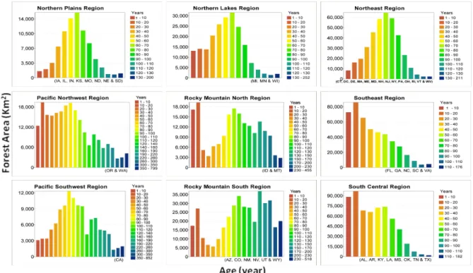
Fig. 4. The forest age distributions in different regions of Continental US (the histograms are placed in this figure as much as possible
corresponding to their geographical positions).
Fig. 5. Forest age distributions of the Southern Alaska of the US and regions of Canada (the histograms are placed in this figure as much as
possible corresponding to their geographical positions).
only forest fragments, and periods of logging as the region was settled. There is less forest area below 20 yr old com-pared with the northern region, which is expected for the southern forests with longer life-cycles and longer time taken for massive canopy openings to have new regeneration.
3.4 The US Pacific Northwest and Southwest regions
Forests in the Pacific Northwest and Southwest regions have the longest life spans of the US though the distribution of age classes tends to younger ages than in the Rocky Moun-tains (Fig. 4). Forest types in the Pacific West are similar to those in the Rocky Mountain regions, though with more local types such as western oak, Hemlock-Sitka spruce and Alder-maple. In the Pacific Northwest, trees can live up to 800 yr, while Pacific Southwest forests have trees up to 1000 yr old (Fig. 4). An abrupt decline of forest age groups older than 100 yr reflects pervasive harvest in late 19th cen-tury (Birdsey et al., 2006) during the westward expansion. In the Pacific West, more than half of old forest areas (more than 100 yr) vanished due to harvest and other disturbances. The area of old growth (generally, 200 yr old or more) in 1992 was estimated to be about 10 million acres (Bolsinger and Waddell 1993), whereas in 1920 there was an estimated 40 million acres of “virgin forest” (Greeley, 1920). There is a distinct contrast in the age pattern of young forests between Pacific Southwest and Northwest regions. The Pacific North-west region has much higher components of young forests due to more intensive regeneration of harvested lands for in-dustrial forests (Figs. 1a and 4), whereas the forests of the Pacific Southwest region were more often left for natural re-covery from disturbances of a century ago and show a natural succession pattern associated with low occurrence of young forests (Fig. 4), indicating that the forests in the region will take many decades to reach maturity.
3.5 The US Southern Alaska region
Inventory-based forest age information in Alaska is quite limited except for the Southeastern Alaska region. The for-est age structure in the region is largely defined by natural disturbances and harvesting in the Tongass National Forest, the largest in the nation (US Forest Service, 2005). The forest longevity is comparable to the Rocky Mountain regions, with species composed of spruce-fir, Hemlock-Sitka Spruce, Fir-Spruce-Mountain Hemlock forests, and a small amount of aspen-birch. There are more old-growth forests than young forests (Fig. 5). There are a few age groups with irregularly higher proportion of area intervened with flatly distributed age groups- the uneven pattern that suggests some large peri-odic disturbances such as fires that happened across the land-scape.
3.6 Canadian Maritime region
Forests in Canada are generally much less affected by human-induced disturbances. The forest age structure in the Canadian Atlantic Maritime region, compared to adjacent Northeast US (NE), fully reflects such a difference. After centuries of farming in this region, few remaining forests are older than 120 yr. However, the percentage of older forests
is still much higher than that in the NE region (Figs. 4 and 5). Forest types and life-spans in this region are similar to the NE region though there are more boreal white and black spruce forests in the northern areas. The region is densely forested with second- and third-growth forests. The domi-nant forest age groups are from 80–120 yr old, on average 40 yr older than the NE region, reflecting the early agricul-ture abundance but without such a heavy harvest of second forests in the early 20th century as occurred in the NE re-gion. Forests in this region also demonstrate a perfect natural successional pattern and the next wave of forest regeneration following various natural disturbances that affected mostly the boreal old growth forests located in the northern areas (Fig. 1a; Kurz and Apps, 1999; Williams and Birdsey, 2003).
3.7 Canadian Great Lakes region
This region is characterized by high coverage of forests and transitional coniferous boreal forests to broad-leaved decid-uous forests. Forest types are similar to the US Northern Lakes region and the NE region. The forest age structure is similar to that in the Atlantic Maritime region, but marked by less remaining trees older than 120 yr (Fig. 5). The suc-cession pattern of forests is not as smooth as the maritime region with apparent traces of frequent natural disturbances, mostly in boreal forests in the north and northwest areas of the region with random disturbance patches and fire scars (Fig. 1a). Most forests younger than 80 yr are distributed rel-atively evenly across age classes except for 20–30 yr old, re-generated after the last spruce-budworm outbreak that caused mortality of canopy trees (Williams and Birdsey, 2003).
3.8 Canadian Prairie region
3.9 Canadian North region
The forests in this region represent the northern component of the Canadian boreal forest belt. A colder climate and shorter growing season nurture more spruce and larch, which dominate the landscape. Along the northern edge the for-est thins into open lichen-woodland with trees growing far-ther apart and smaller in size as the forest stretches towards the treeless tundra. The forest age structure in the region is broken into two cohorts, trees younger than 40 yr old, and trees between 80–120 yr old (Fig. 5). Forest age structure in such a landscape is very much an indicator of periodic and highly variable fire disturbance cycles (Kurz and Apps, 1999). However, for this region, the data are particularly poor. The lack of forests aged from 40–80 yr indicates a lack of disturbance events for a long period, 1920–1960, which is unlikely. It is possible that this age cohort is missing be-cause there is little data available for the region before 1959, and also because the average ages (75–120 yr) were used to assign the pixels to age classes based on the disturbance oc-currence intervals in each ecoregion (see Methods).
3.10 Canadian Pacific region
This region is characterized by the temperate rainforest, which is adapted to the steep cliffs and rugged coastlines of this area. The region has higher rainfall and fewer fires than other regions in Canada. As a result, trees in the temper-ate rainforest are often much older than those found in the boreal forest (Fig. 1a). Forests in the lower seaward slopes of the Coast Mountains include old growth cedar and Sitka spruce, while the steep hill slopes are habitat to western hem-lock, balsam, red cedar and spruce. In the areas between the Rockies and the Central Plateau including several val-leys, forest types resemble the coastal region, characterized by Douglas fir, western white pine, western larch, Lodgepole and ponderosa pine, and trembling aspen. Engelmann spruce and alpine fir are found in the subalpine region. The for-est age structure shows a great amount of old-growth forfor-ests (>150 yr) still remaining in the region (Fig. 5). However, harvests between later 19th and early 20th centuries replaced old-growth forests with younger trees. Since then, forest age classes smoothly decline from 120 yr to 20 yr old, related to managed harvesting and reforestation in this most impor-tant timber industrial land of Canada. A high component of forests less than 20 yr old is the result of combined effects, recent severe outbreaks of insects in the region (Kurz et al., 2008b), harvesting, and regeneration of new plantations. 3.11 Summary of regional analysis
The above analyses based on characteristics of the forest age map and the current forest age distribution patterns in differ-ent regions of the US and Canada clearly show the depen-dence of current age structure on disturbances of the past,
both by natural events and human activities. The information is remarkably consistent with our knowledge about the land-use history and forest past in North America since European colonists arrived in North America (Sisk, 1998). Forest ages certainly carry the disturbance legacy and are excellent sur-rogates for addressing disturbance impacts on forests. Our analysis shows that forests in the US bear much deeper and broader human footprints than in Canada, that most forests in the US were disturbed in the last two centuries, except some inaccessible areas in the Rocky Mountains and Alaska, and that some old-growth remains in the Pacific Northwest and Southwest. In Canada, industrial timber harvest is quite intensive in some areas of boreal and temperate rainforests. However, because of Canada’s immense forest lands and frequent and wide-spread natural disturbances, particularly wildfires, forested lands are distinctly marked by natural dis-turbances with the exception of the Pacific Region. On av-erage in Canada, the annual burned area is more than three times the area of current annual industrial timber harvest, and the burned area is even more widespread in bad fire years (Stocks et al., 2003). Just the opposite is true for the US where the impact of timber harvest is several times that of the impact of natural disturbances.
4 Application of forest age map in forest carbon studies
Because forest disturbance and regrowth profoundly affect forest capacity for sequestering and storing carbon, our continent-wide spatial data of forest age distribution can be used for improving estimates of forest carbon stock and flux in North America, and can also be used as a reference for assessing the future forest carbon balance and potential, re-gardless of whether the estimation approach is empirical or model based. Though there are many possible applications of this valuable information to forest carbon studies, here we describe a few potential uses to provoke further ideas. 4.1 Using the age map to analyze impacts of forest
management on carbon sequestration
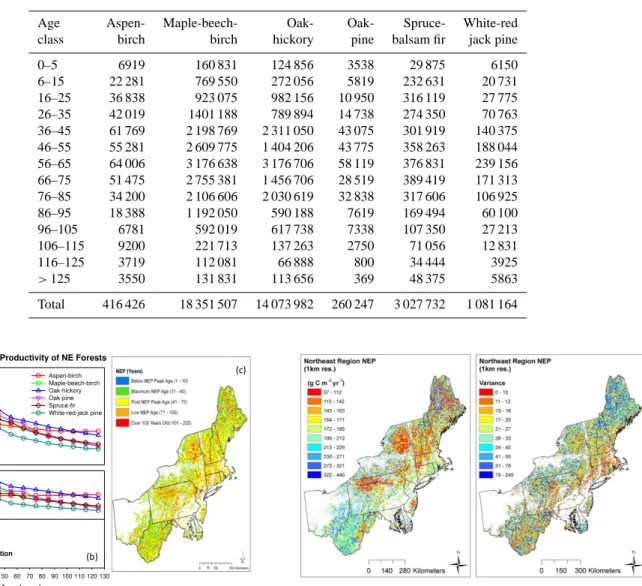
Table 2. Area (ha) by forest type and age class for the Northeast US.
Age Aspen- Maple-beech- Oak- Oak- Spruce- White-red class birch birch hickory pine balsam fir jack pine
0–5 6919 160 831 124 856 3538 29 875 6150
6–15 22 281 769 550 272 056 5819 232 631 20 731
16–25 36 838 923 075 982 156 10 950 316 119 27 775
26–35 42 019 1401 188 789 894 14 738 274 350 70 763 36–45 61 769 2 198 769 2 311 050 43 075 301 919 140 375 46–55 55 281 2 609 775 1 404 206 43 775 358 263 188 044 56–65 64 006 3 176 638 3 176 706 58 119 376 831 239 156 66–75 51 475 2 755 381 1 456 706 28 519 389 419 171 313 76–85 34 200 2 106 606 2 030 619 32 838 317 606 106 925
86–95 18 388 1 192 050 590 188 7619 169 494 60 100
96–105 6781 592 019 617 738 7338 107 350 27 213
106–115 9200 221 713 137 263 2750 71 056 12 831
116–125 3719 112 081 66 888 800 34 444 3925
>125 3550 131 831 113 656 369 48 375 5863
Total 416 426 18 351 507 14 073 982 260 247 3 027 732 1 081 164
Net Ecosystem Productivity of NE Forests
NEP (Mg C h
a
-1yr -1)
0.0 0.5 1.0 1.5 2.0 2.5 3.0 3.5 4.0 4.5 5.0
Aspen-birch Maple-beech-birch Oak-hickory Oak-pine Spruce-fir White-red-jack pine
Age (year)
0 10 20 30 40 50 60 70 80 90 100 110 120 130
NEP (Mg C h
a
-1 y
r
-1)
-3.0 -2.5 -2.0 -1.5 -1.0 -0.5 0.0 0.5 1.0 1.5 2.0 2.5 3.0
Aforestation
Reforestation
(a)
(b)
(c)
Fig. 6. Mean annual net ecosystem productivity of Northeast
re-gion forests based on forest inventory data: (a) from afforestation sites; (b) from deforestation sites, NEP loss from woody product is not counted in the initial year, and (c) Northeastern forests with different NEP levels related to age.
an estimate of average annual NEP (Mg C ha−1yr−1)for the interval. When combined across all age classes, the resulting curve shows the pattern of NEP over time (Fig. 6a and b).
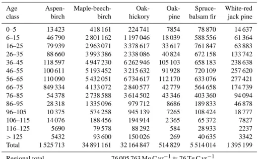
From the age map, we estimate the area by forest type and age (Table 2) and then multiply the estimated area of each category with the corresponding NEP to produce regional NEP estimates (Table 3a and b). A regional NEP map can also be presented by co-registering the age map, forest type map and age-related NEP values (Fig. 7) (Pan et al., 2010). Because of uncertainty in the forest age map, the variance in NEP inherited from that source can also be evaluated. For the whole region, the uncertainty in NEP ranges from 2.3–
Fig. 7. Average Net Ecosystem Production (gC m−2yr−1)of the US Northeastern forests and the variation inherited from the age deviation.
(Ollinger et al., 2002). There is 25%–42% lower NEP (de-pendent on forest types) on reforestation sites that follow harvest or other disturbances because of the loss of carbon from forest floor and soils, which is different from afforested sites where soil carbon typically increases to recover de-pleted pools from previous agriculture use (e.g. Post and Kwon, 2000). In reforestation sites, post-disturbance NEP dynamics depend on disturbance types and slash treatment methods. However, our estimates of the reduced NEP re-flect regional average patterns and are not specific to either industrial forestry or areas prone to natural disturbances. As a result, annual NEP in the New England forests under the current age structure is between 60–76 Tg C which compares favorably with recent estimates of annual changes in carbon stocks from repeated inventories (US Department of Agri-culture, 2008). In total, the carbon accumulation from re-forestation sites is about 20% lower than afre-forestation sites; however we did not count carbon in harvested wood from the reforestation sites, which could largely compensate for the lower carbon accumulation in reforestation sites.
Forest age can be a good indicator of management oppor-tunity. When compared with a standard growth curve, forest age can indicate whether the stand is aggrading or degrad-ing, giving the land manager an indication of the kind of treatments that can be applied if the manager is interested in changing the rate of carbon sequestration or increasing the stock of carbon on a landscape. Continuing the previous ex-ample for New England, we show the deviation from maxi-mum NEP for each forest grid cell of the Northeast and indi-cate whether this deviation is because the forest is younger or older than the age of maximum NEP (Fig. 6c). If the manager is interested in maximizing NEP, it may be determined that forests younger than the age of maximum NEP could be left alone because carbon sequestration will increase without any intervention, and that forests older than the age of maximum NEP may be considered for thinning to reduce stand density to an effectively younger age. If the manager is interested in increasing the stock of carbon on a landscape, the map may be used to identify forests that are already at high stocking levels and would require protection from disturbance, and to identify forest areas that could be left to grow older. As shown by the regional age distributions described in the pre-vious section, some combination of maximizing NEP and maximizing C stocks is likely to emerge in practice over large regions, considering that forests are not only managed for carbon but also for many other purposes such as timber pro-duction and recreation. Note that in this simple exercise we are not recommending a specific approach to increase carbon sequestration or carbon stocks. A full assessment of man-agement opportunities is much more complicated and needs to consider factors such as emissions and retention of C in harvested wood, the energy inputs for stand treatments, and impacts on soil C, to name a few. Our results clearly show that after disturbances (referring to reforested sites) forests have reduced total NEP (Table 3) because of carbon losses in
the earlier recovery stages. The age map combined with the mapped productivity provides a first-level spatial analysis of the state of the forest system, which may then be expanded to a full carbon accounting and management recommendations. 4.2 Using the age map to improve carbon estimation by
terrestrial models
Process-based biogeochemical models are important tools to estimate terrestrial carbon budgets (Sitch et al., 2008). A very unique function of such “mechanistic” models is the ability in a diagnostic sense to interpret temporal and spatial patterns of forest C dynamics and partition the effects of var-ious climatic drivers and different environmental variables, which are not always identifiable by experimental and obser-vation approaches (Pan et al., 2009). Therefore, terrestrial carbon models can serve as powerful methods to integrate and expand our knowledge of complex interactive effects of multiple environmental changes on forest carbon dynamics. Terrestrial carbon models are continuously improving by re-ducing uncertainty in estimation and prediction, and by im-proving input data layers, model formulas and parameters (Pan et al., 2006).
Currently, many land-based terrestrial carbon models are not capable of reflecting the impact of land disturbances be-cause spatially-explicit historical data at landscape scales is lacking. Therefore, most models represent ecosystem dy-namics at equilibrium conditions (Canadell et al., 2007a). However, with the availability of spatial forest age data and its ability to simply represent historical disturbance legacy, we can improve terrestrial biogeochemistry models by us-ing age cohorts and incorporation of forest growth curves (Fig. 6a and b), making the models capable of simulating for-est regrowth dynamics as the consequences of the impact of land-use, human and natural disturbances (Pan et al., 2002), even if they may not able to separate direct and indirect ef-fects.
In a Canada-wide forest carbon cycle study using a mech-anistic ecosystem model with consideration of both distur-bance (mostly fire) and lack of disturdistur-bance (climate, CO2
Table 3a. Area-weighted NEP (Mg C yr−1)by forest type for the Northeast US (based on the mean values of NEP (Mg C ha−1yr−1)from afforestation sites.)
Age Aspen- Maple-beech- Oak- Oak- Spruce- White-red class birch birch hickory pine balsam fir jack pine
0–5 13 423 418 161 224 741 7854 78 870 14 637
6–15 46 790 2 801 162 1 197 046 18 039 588 556 61 364 16–25 79 939 2 963 071 3 378 617 33 617 761 847 63 883 26–35 88 660 3 993 386 2 338 086 40 824 672 158 133 742 36–45 118 597 4 947 230 6 262 946 105 103 658 183 238 638 46–55 100 611 5 193 452 3 215 632 91 928 720 109 257 620 56–65 110 090 5 432 051 6 734 617 112 170 633 076 277 421 66–75 849 334 4 133 072 2 840 577 42 779 564 658 174 739 76–85 54 378 2 738 588 3 614 502 43 346 403 360 94 094
86–95 28 318 1 335 096 979 712 8686 189 833 46 878
96–105 10 375 574 258 945 139 7265 108 424 18 777
106–115 14 076 188 456 194 914 2 365 65 372 7827
116–125 5690 79 578 88 292 584 28 933 2237
>125 5432 93 600 150 026 269 40 635 3342
Total 1 525 713 34 891 161 32 164 847 514 829 5 514 014 1 395 199
Regional total 76 005 763 Mg C yr−1≈76 Tg C yr−1
Table 3b. Area-weighted NEP (Mg C yr−1) by forest type for the Northeast US (based on the mean values of NEP (Mg C ha−1yr−1) from reforestation sites).
Age Aspen- Maple-beech- Oak- Oak- Spruce- White-red class birch birch hickory pine balsam fir jack pine
0–5 −1661 −308 796 −254 706 −6793 −42 423 615
6–15 19 162 961 938 609 405 5004 90 726 33 792
16–25 52 678 1 938 458 2 347 353 21 134 410 955 41 663 26–35 65 970 3 096 625 1 879 948 30 508 469 139 91 284 36–45 90 800 4 001 760 5 338 526 83 566 486 090 174 065 46–55 81 263 4 358 324 2 864 580 76 606 562 473 188 044 56–65 93 449 4 764 957 6 162 810 97 640 512 490 217 632 66–75 75 668 3 719 764 2 665 772 38 216 478 985 142 190 76–85 50 616 2 527 927 3 492 665 39 734 362 071 83 402
86–95 27 214 1 275 494 950 203 8229 176 279 42 671
96–105 10 172 562 418 932 784 7045 104 130 17 961
106–115 13 892 184 022 193 541 2310 63 240 7699
116–125 5 653 79 578 87 623 584 28 933 2 159
>125 5396 93 600 148 889 269 40 635 3225
Total 590 272 27 256 068 27 419 392 404 050 3 743 717 1 046 399
ecosystems over a landscape, they can provide the bench-mark for the modeling studies (Pan et al., 2010). Based on the average NEP, it is a very reasonable to use an ecosys-tem model to generate annual anomalies and spatial effects of soils and climate on NEP by incorporating more driving variables, and to produce more spatially and temporally ex-plicit NEP estimates (Chen et al., 2003).
4.3 Using the age map to improve land constraints on atmospheric inversion models
Several recent publications show a full analysis of the global carbon cycle with comprehensive consideration of carbon fluxes or stock changes in the atmosphere, ocean, and land (Le Qu´er´e et al., 2009, Canadell et al., 2007b). In such analyses, the carbon exchange between the ocean and land surfaces with the atmosphere is estimated based on global transport inversion using observations of CO2concentration
in the atmosphere (Peters et al., 2007). Usually, inverse models are not well constrained because of an insufficient number of CO2 observation sites in the global monitoring
network. Simulated carbon fluxes from lands and oceans with additional consideration of other surface observations are needed to provide constraints to the inverse modeling to obtain meaningful results. However, such inverse mod-eling could suffer great uncertainty from small-scale struc-ture of the fluxes due to spatial heterogeneity, particularly for the regions lacking observations such as the tropical ar-eas (Stephens et al., 2007).
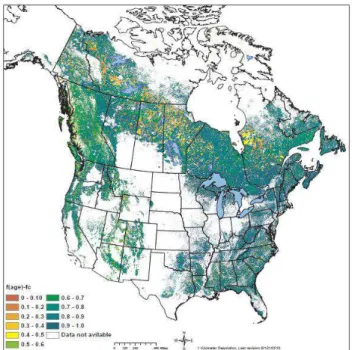
One way to improve the inversion estimates is to provide better land-surface flux constraints. The a priori carbon flux fields from lands used for the inversion constraint are of-ten obtained from ecosystems models validated at discrete sites using measurements such as eddy covariance (Deng et al., 2007; Peters et al., 2007). None of these surface flux fields used for constraining the inversions has so far consid-ered forest carbon dynamics associated with forest age. The flux tower data have shown the obvious relationship between net ecosystem productivity (NEP) and forest stand age, in-dicating that the carbon flux over forests is closely related to forest age (Chen et al., 2003; Law et al., 2003). In order to capture the large scale regional patterns of the carbon flux associated with the disturbance and regrowth cycle and to es-timate the first order effect of forest age on NPP and therefore NEP, the continent-wide forest age map is used for develop-ing a forest age factor map (Fig. 8) (Deng et al., 2011), in which the age factor was calculated as a scalar based on a generalized NPP-age relationship (Chen et al., 2003). The generalized NPP-age relationship has a similar temporal pat-tern to those shown in NEP curves (Fig. 6a and b), when the heterotrophic respiration is assumed to be constant. The re-lationship is normalized against the maximum NPP value, so that the normalized NPP varies between zero and one. In the generalized NPP-age relationship, the age at which the maximum NPP occurs depends on the mean annual air
tem-Fig. 8. Forest age factor derived from the forest age map (tem-Fig. 1a)
useful for constraining atmospheric inverse modeling of the bio-sphere carbon flux.
perature at each pixel (Chen et al., 2003), considering the fact that forests grow faster and reach the maximum NPP earlier under warmer climates. Other factors, such as precipitation, soil and topography, may influence the magnitude of NPP but are assumed to have no influence on the timing of the maximum NPP occurrence.
Figure 8 shows the distribution of the age factor (normal-ized NPP value) at the continental scale determined by the age map (Fig. 1a) and the mean annual air temperature (Deng et al., 2011). Low values (warm tone, i.e. yellow to red) in-dicate low productivity relative to its own life cycle either due to young or very old ages, where NPP is most likely smaller than the heterotrophic respiration (NEP<0). High values (cold tone, i.e. green to blue) suggests high produc-tivity, where NPP is most likely greater than heterotrophic respiration (NEP>0). The fact that the overall distribution over the continent has a cold tone suggests that the forest age structure in North America is in favor of carbon sinks. The age factor map has been used to introduce a priori co-variance as an additional constraint for an atmospheric inver-sion (Deng et al., 2011). The results show that at the sub-continental level, the inversed carbon fluxes are better cor-related with the fluxes derived from the eddy covariance and MODIS when the age factor is used. As reliable CO2
5 Discussion and conclusion
Ground-based and spatially explicit forest age data provide valuable information for improving forest carbon estimates, evaluating disturbance impacts, and predicting forest carbon sequestration potential in the next few decades as forests nat-urally proceed to reach maturity or start new succession. However, there are limitations of an age map for charac-terizing succession and carbon sequestration. Assigning an age to a forest is an inexact process. Trees in many if not most forests have different ages, so the assigned age is typ-ically an average age unless there is a very distinct dis-turbance and regeneration activity such as a clear-cut fol-lowed by a plantation establishment (Bradford et al., 2008). Forests undisturbed for long periods of time tend to develop an uneven-aged stand structure as canopy gaps become filled with younger trees (Luyssaert et al., 2008). Many natural disturbances do not kill all of the trees in a forest stand, so the regenerating trees are often growing amongst a residual number of older trees. And natural regeneration may be a slow process such that the new trees may span a range of ages over several decades (Pregitzer and Euskirchen, 2004). Because of the nature of these disturbance and regeneration processes, there is a difference between age and time since disturbance (Bradford et al., 2008). In many cases, an ob-served tree age may be a poor predictor of time since dis-turbance, and depending on how this information is used in models, estimates of carbon stocks or fluxes may have sig-nificant errors.
Tree age data are not available everywhere in North Amer-ica. Some regions are not very well covered by forest in-ventories, such as interior Alaska and the northern part of Canada. It is important to acknowledge the uncertainty and inaccuracy of the age map because of limitations of data sources and methodologies, particularly, inconsistency of age-related data between Canada and the US (Table 1). For instance, for the US, the disturbance information derived from remote sensing only covers 10 yr (1990–2000), so the impact of disturbances that occurred before (or after) then could be missed in the age map if the inventory data does not pick up all disturbance effects. This can be particularly true for disturbance-prone regions in the western US where wildfires occur at a high frequency. In Canada, a big prob-lem is for the massive area of northern boreal forests that have little ground-based inventory data to constrain the as-signment of ages to pixels. Accordingly, the age map is only a metadata-based result, given the fact that the forest age is represented by a single value in a pixel of 1 km resolution that more likely contains a mix of ages. The map is most ap-propriate for large-scale studies and should be used very cau-tiously for geographic areas smaller than those described in this paper. The companion map of standard deviation for the age map should be considered for evaluating uncertainty in application of the age map for studying regional carbon, wa-ter and nutrient cycles. For the areas with high uncertainty in
age estimates such as British Columbia and US west coasts (Fig. 1b) where a greater spatial heterogeneity of forest age cohorts occurs on the landscape, it is particularly critical to choose a proper scale for using the product and perhaps nec-essary for collecting local data for validation.
We have shown that age is a convenient indicator of forest development status after disturbance, can be easily related to ability of forests to sequester and store carbon, and can support improvements in analysis and modeling techniques. However, age is not the only factor affecting carbon stocks and rate of C uptake. Climate, atmospheric CO2, air
pol-lution, N deposition, fertilization, and other factors may be significant (Canadell et al., 2007a; Pan et al., 2009). The data from forest inventories that underlie the carbon stock and NEP curves used in this analysis reflects the aggregate effect of these factors over the region of interest. Therefore, results may be accurate even if the effects of all of the con-tributing factors are not individually estimated. Finally, for-est age maps may be used in conjunction with remote sens-ing data for drivsens-ing predictive models of forest dynamics. Although signals from optical remote sensors tend to satu-rate at the time of tree crown closure, lidar and radar sensors can extend the data to older age classes and higher biomass densities. Models driven by remote sensing, such as CASA (Potter et al., 1993), may benefit from good characterization of forest age in terms of improving the accuracy of gridded estimated of productivity and carbon stocks.
Acknowledgements. Yude Pan and Richard Birdsey acknowledge
support from NASA grants (NNH09AM30I and NNH08AH971) and the Forest Service Global Change Research Program. Jing Chen acknowledges support from the Canadian Carbon Program funded by the Canadian Foundation of Climate and Atmospheric Sciences, as well as funding support from US Department of Agri-culture and Natural Science and Engineering Council of Canada. We are thankful to John Hom for his useful methodological advice. We owe great thanks to three anonymous reviewers and the editor for their critical and constructive comments, which have substantially improved this manuscript.
Edited by: M. Bahn
References
Amiro, B. D. and Chen, J. M.: Forest-fire-scar dating using SPOT-VEGETATION for Canadian ecoregions, Can. J. Forest Res., 33, 1116–1125, 2003.
Amiro, B. D., Todd, J. B., Wotton, B. M., Logan, K. A., Flannigan, M. D., Stocks, B. J., Mason, J. A., Martell, D. L., and Hirsch, K. G.: Direct carbon emissions from Canadian forest fires, 1959– 1999. Can. J. For. Res. 31, 512–525, 2001.
BC Ministry of Forests: Annual Report of the Ministry of Forests 2002/03, http://www.for.gov.bc.ca/mof/annualreports.htm, 2003. Bechtold, W. A. and Patterson, P. L. (Eds.): The enhanced Forest In-ventory and Analysis program-national sampling design and esti-mation procedures, Gen. Tech. Rep., SRS-80, Asheville, NC, US Department of Agriculture, Forest Service, Southern Research Station, p. 85, 2005.
Birdsey, R. A., Jenkins, J. C., Johnston, M., Huber-Sannwald, E., Amero, B., de Jong, B., Barra, J. D. E., French, N., Garcia-Oliva, F., Harmon, M., Heath, L. S., Jaramillo, V. J., Johnsen, K., Law, B. E., Mar´ın-Spiotta, E., Masera, O., Neilson, R., Pan, Y., and Pregitzer, K. S.: North American Forests, in: The First State of the Carbon Cycle Report (SOCCR): The North American Car-bon Budget and Implications for the Global CarCar-bon Cycle. A Report by the US Climate Change Science Program and the Sub-committee on Global Change Research, edited by: King, A. W., Dilling, L., Zimmerman, G. P., Fairman, D. M., Houghton, R. A., Marland, G., Rose, A. Z., and Wilbanks, T. J.: National Oceanic and Atmospheric Administration, National Climatic Data Center, Asheville, NC, USA, 117–126, 2007.
Birdsey, R. A. and Heath, L. S.: Carbon changes in US forests, in: Productivity of America’s Forests and Climate Change, edited by: Joyce, L. A., Gen. Tech. Rep. RM-271, Fort Collins, CO, US Department of Agriculture, Forest Service, Rocky Mtn. Forest and Range Exp. Station, 56–70, 1995.
Birdsey, R. A. and Lewis, G. M.: Current and historical trends in use, management, and disturbance of US forestlands, in: The potential of US forest soils to sequester carbon and mitigate the greenhouse effect, edited by: Kimble, J. M., Linda, H. S., and Birdsey, R. A., New York, CRC Press LLC, 15–33, 2003. Birdsey, R. A. and Schreuder, H. T.: An overview of forest
inven-tory and analysis estimation procedures in the Eastern United States – with an emphasis on the components of change, Gen. Tech Rep. RM-214, Fort Collins, CO, US Department of Agri-culture, Forest Service, Rocky Mountain Forest and Range Ex-periment Station, p. 11, 1992.
Birdsey, R., Pregitzer, K., and Lucier, A.: Forest carbon manage-ment in the United States 1600–2100, J. Environ. Qual., 35, 1461–1469, 2006.
Bolsinger, C. L. and Waddell, K. L.: Area of old-growth forests in California, Oregon, and Washington, Resour. Bull. PNW-RB-197, Portland, OR, US Department of Agriculture, Forest Ser-vice, Pacific Northwest Research Station, p. 26, 1993.
Bradford, J. B., Birdsey, R. A., Joyce L. A., and Ryan, M. G.: Tree age, disturbance history, and carbon stocks and fluxes in subalpine Rocky Mountain forests, Glob. Change Biol., 14(12), 2882–2897, 2008.
Canadell, J. G., Pataki, D., Gifford, R., Houghton, R. A., Lou, Y., Raupach, M. R., Smith, P., and Steffen, W.: Saturation of the ter-restrial carbon sink, in: Ecosystems in a Changing World, edited by: Canadell, J. G., Pataki, D., and Pitelka, L., The IGBP Series, Springer-Verlag, Berlin Heidelberg, 59–78, 2007a.
Canadell, J. G., Le Qu´er´e, C., Raupach, M. R., Field, C. B., Buite-huis, E. T., Ciais, P., Conway, T. J., Houghton, R. A., and Mar-land, G.: Contributions to accelerating atmospheric CO2growth
from economic activity, carbon intensity, and efficiency of natu-ral sinks, PNAS, Proc. Nat. Aca. Sci., 104, 18866–18870, 2007b. Chen, J. M. and Cihlar, J.: A hotspot function in a simple bidi-rectional reflectance model for satellite applications, J. Geophys.
Res., 102, 25907–25913, 1997.
Chen, J. M., Ju, W., Cihlar, J., Price, D., Liu, J., Chen, W., Pan, J., Black, T. A., and Barr, A.: Spatial distribution of carbon sources and sinks in Canada’s forests based on remote sensing, Tellus B, 55(2), 622–642, 2003.
Deng, F., Chen, J. M., Yuen, C.-W., Ishizawa, M., Mo, G., Higuchi, K., Chan, D., Chen, B., and Maksyutov, S.: Global monthly CO2
flux inversion with focus over North America, Tellus, 59B, 179– 190, 2007.
Deng, F., Chen, J. M., Pan, Y., Peter W., Birdsey, R., McCullough, K., and Xiao, J.: Using forest stand-age to constrain an inverse North American carbon flux estimate, Global Biogeochem. Cy., submitted, 2011.
Donnegan, J. A., Veblen, T. T., and Sibold, J. S.: Climatic and hu-man influences on fire history in Pike National Forest, Central Colorado, Can. J. For. Res., 31, 1526–1539, 2001.
Fedkiw, J.: The evolving use and management of the nation’s forests, grasslands, croplands, and related resources, USDA For-est Service, Gen. Tech. Rep. RM-175, Ft. Collins, CO, p. 66, 1989.
Food and Agriculture Organization (FAO): Global forest Resources Assessment, Rome, Italy, p. 320, 2005.
Gallant, A. L., Hansen, A. J., Councilman, J. S., Monte, D. K., and Betz, D. W.: Vegetation dynamics under fire exclusion and log-ging in a Rocky Mountain watershed, 1856–1996, Ecol. Appl., 13(2), 385–403, 2003.
Greeley, W. B.: Timber depletion, lumber prices, lumber exports, and concentration of timber ownership, US Department of Agri-culture, Forest Service, Report on Senate Resolution, 311, p. 39, 1920.
He, L., Chen, J. M., Zhang, S, Gomez, G., Pan, Y., McCullough, K., and Birdsey, R.: Normalized Algorithm for Mapping and Dating Forest Disturbances and Regrowth for the United States, Journal of Applied Earth Obsevation and Geoinformation, in press, 2011. Hollinger, D. Y., Aber, J., Dail, B., Davidson, S. M., Goltz, H., and Hughes, H.: Spatial and temporal variability in forest-atmosphere CO2exchange, Glob. Change Biol., 10, 1689–1706,
2004.
Keeling, E. G., Sala, A., and DeLuca, T. H.: Effects of fire ex-clusion on forest structure and composition in unlogged pon-derosa pine/Douglas-fir forests, Forest Ecol. Manag., 237, 418– 428, 2006.
Kurz, W. A. and Apps, M. J.: An analysis of future carbon budgets of Canadian boreal forests, Water Air Soil Poll., 82, 321–331, 1995.
Kurz, W. A. and Apps, M. J.: A 70-year retrospective analysis of carbon fluxes in the Canadian forest sector, Ecol. Appl., 9, 526– 547, 1999.
Kurz, W. A., Stinson, G., Rampley, G. J., Dymond, C. C., Neilson, E. T.: Risk of natural disturbances makes future contribution of canada’s forests to the global carbon cycle highly uncertain, Proc. Nat. Aca. Sci., 105(5), 1551–1555, 2008a.
Kurz, W. A., Dymond, C. C., Stinson, G., Rampley, G. J., Neil-son, E. T., Carroll, A. L., Ebata, T., and Safranyik, L.: Mountain pine beetle and forest carbon feedback to climate change, Nature, 452(24), 987–990, 2008b.
Law, B. E., Sun, O. J., Campbell, J., Vantuyl, S., and Thornton, P. E.: Changes in carbon storage and fluxes in a chronosequence of ponderosa pine, Glob. Change Biol., 9, 510–524, 2003. Le Qu´er´e, C., Raupach, M. R., Canadell, J. G., Marland, G., Bopp,
L., Ciais, P., Conway, T. J., Doney, S. C., Feely, R. A., Foster, P., Friedlingstein, P., Gurney, K., Houghton, R. A., House, J. I., Huntingford, C., Levy, P. E., Lomas, M. R., Majkut, J., Metzl, N., Ometto, J. P., Peters, G. P., Prentice, I. C., Randerson, J. T., Running, S. W., Sarmiento, J. L., Schuster, U., Sitch, S., Taka-hashi, T., Viovy, N., van der Werf, G. R., and Woodward, F. I.: Trends in the sources and sinks of carbon dioxide, Nat. Geosci., 2, 831–836, 2009.
Lowe, J. J., Power, K., and Gray, S. L.: Canada’s forest inven-tory 1991: the 1994 version-technical supplement, Canada Forest Service, Information Report BC-X-362E, 1996.
Luyssaert, S., Schulze, E.-D., B¨orner, A., Knohl,A., Hessenm¨oller, D., Law, B. E., Ciais, P., and Grace, J.: Old-growth forests as global carbon sinks, Nature, 455, 213–215, 2008.
MacCleery, D. W.: American forests – a history of resiliency and recovery, FS-540, USDA Forest Service, Washington, DC, p. 58, 1992.
Masek, J. G., Huang, C., Wolfe, R., Cohen, W., Hall, F., Kutler, J., and Nelson, P.: North American forest disturbance mapped from a decadal Landsat record, Remote Sens. Environ., 112, 2914– 2926, 2008.
Nabuurs, G. J., Masera, O., Andrasko, K., Benitez-Ponce, P., Boer, R., Dutschke, M., Elsiddig, E., Ford-Robertson, J., Frumhoff, P., Karjalainen, T., Krankina, O., Kurz, W. A., Matsumoto, M., Oy-hantcabal, W., Ravindranath, N. H., Sanz Sanchez, M. J., and Zhang, X.: Forestry, in: Climate Change 2007: Mitigation, Con-tribution of Working Group III to the Fourth Assessment Report of the Intergovernmental Panel on Climate Change, edited by: Metz, B., Davidson, O. R., Bosch, P. R., Dave, R., and Meyer, L. A., Cambridge University Press, Cambridge, United Kingdom and New York, NY, USA, 2007.
Ollinger, S. V., Aber, J. D., Reich, P. B., and Freuder, R. J.: Interac-tive effects of nitrogen deposition, tropospheric ozone, elevated CO2land use history on the carbon dynamics of northern
hard-wood forests, Glob. Change Biol., 8, 545–562, 2002.
Pan, Y., McGuire, A. D., Melillo, J. M., Kicklighter, D. W., Sitch, S., and Prentice, I. C.: A biogeochemistry-based successional model and its application along a moisture gradient in the conti-nental United States, J. Veg. Sci., 13, 369–380, 2002.
Pan, Y., Birdsey, R., Hom, J., McCullough, K., and Clark, K.: Im-proved estimates of net primary productivity from MODIS satel-lite data at regional and local scales, Ecol. Appl., 16(1), 125–132, 2006.
Pan, Y., Birdsey, R., Hom, J., and McCullough, K.: Separating Effects of Changes in Atmospheric Composition, Climate and Land-use on Carbon Sequestration of US Mid-Atlantic Temper-ate Forests, Forest Ecol. Manag., 259, 151–164, 2009.
Pan, Y., Birdsey, R., McCullough, K., Chen, J. M., and Wayson, C.: The benchmark for carbon models: Net ecosystem produc-tivity of US forests estimated from forest inventory data, AIMES Open Science Conference, Earth System Science 2010: Global Change, Climate and People, Edinburgh, Abstract Book, p. 50, 2010.
Penner, M., Power, K., Muhairwe, C., Tellier, R., and Wang, Y.: Canada’s forest biomass resources: deriving estimates from
Canada’s forest inventory, Information Report BC-X-370, Pacific Forestry Centre, Canadian Forest Service, Natural Resources Canada, 1997.
Peters, W., Jacobson, A. R., Sweeney, C., Andrews, A. E., Conway, T. J., Masarie, K., Miller, J. B., Bruhwiler, L. M. P., P´etron, G., Hirsch, A. I., Worthy, D. E. J., van der Werf, G. R., Randerson, J. T., Wennberg, P.O., Krol, M. C., and Tans, P. P.: An atmospheric perspective on North American carbon dioxide exchange: Car-bonTracker, Proc. Nat. Aca. Sci., 104(48), 18925–18930, 2007. Post, W. M. and Kwon, K. C.: Soil carbon sequestration and
land-use change: processes and potential, Glob. Change Biol., 6, 317– 327, 2000.
Potter, C. S., Ranserson, J. T., Field, C. B., Matson, P. A., Vitousek, P. M., Mooney, H. A., and Jlooster, S. A.: Terrestrial ecosystem production: a process model based on global satellite and surface data, Global Biogeochem. Cy., 7, 811–841, 1993.
Pregitzer, K. and Euskirchen, E.: Carbon cycling and storage in world forests: biome patterns related to forest age, Glob. Change Biol., 10, 2052–2077, 2004.
Ruefenacht, B., Finco, M. V., Nelson, M. D., Czaplewski, R., Helmer, E. H., Blackard, J. A., Holden, G. R., Lister, A. J., Sala-janu, D., Weyermann, D., and Winterberger, K.: Conterminous US and Alaska Forest Type Mapping Using Forest Inventory and Analysis Data, Photogramm. Eng. Rem. S., 74(11), 1379–1388, 2008.
Smith, J. E., Heath, L. S., Skog, K. E., and Birdsey, R. A.: Meth-ods for Calculation Forest Ecosystem and Harvested Carbon with Standard Estimates for Forest Types of the United States, Gen. Tech. Rep. NE-343, Newtown Square, PA, USDA, Forest Ser-vice, Northeastern Research Station, 216, 2006.
Sisk, T. D. (Ed.): Perspectives on the land use history of North America: a context for understanding our changing environment, US Geological Survey, Biological Resources Division, Biologi-cal Science Report USGS/BRD/BSR-1998-0003, p. 104, 1998. Sitch, S., Huntingford, C., Gedney, N., Levy, P. E., Lomass, M.,
Piao, S. L., Betts, R., Ciais, P., Cox, P., Friedlingstein, P., Jones, C. D., Preentice, I. C., and Woodward, F. I.: Evaluation of the ter-restrial carbon cycle, future plant geography and climate-carbon cycle feedbacks using five Dynamic Global Vegetation Models (DGVMs), Glob. Change Biol., 14, 2015–2039, 2008.
Smoyer-Tomic, K. E., Justine, Klaver, J. D. A., Soskolne, C. L., and Spady, D. W.: Health Consequences of Drought on the Canadian Prairies, EcoHealth, 1 (Suppl. 2), 144–154, 2004.
Stephens, B. B., Gurney, K. R., Tans, P. P., Sweeney, C., Peters, W., Bruhwiler, L., Ciais, P., Ramonet, M., Bousquet, P., Nakazawa, T., Aoki, S., Machida, T., Inoue, G., Vinnichenko, N., Lloyd, J., Jordan, A., Heimann, M., Shibistova, O., Langenfelds, R. L., Steele, L. P., Francey, R. J., and Denning, A. S.: Weak Northern and Strong Tropical Land Carbon Uptake from Vertical Profiles of Atmospheric CO2, Science, 316, 1732–1735, 2007.
Stocks, B. J., Mason, J. A., Todd, J. B., Bosch, E. M., Wotton, B. M., Amiro, B. D., Flannigan, M. D., Hirsch, K. G., Lo-gan, K. A., Martell, D. L., and Skinner, W. R.: Large forest fires in Canada, 1959–1997, J. Geophys. Res., 108(D1), 8149, doi:10.1029/2001JD000484, 2003.
US Forest Service: Land areas of the National Forest System, FS-383, Washington, DC, p. 154, 2005.