www.hydrol-earth-syst-sci.net/17/4453/2013/ doi:10.5194/hess-17-4453-2013
© Author(s) 2013. CC Attribution 3.0 License.
Hydrology and
Earth System
Sciences
A paradigm shift in stormflow predictions for active tectonic regions
with large-magnitude storms: generalisation of catchment
observations by hydraulic sensitivity analysis and insight into
soil-layer evolution
Makoto Tani
Laboratory of Forest Hydrology, Graduate School of Agriculture, Kyoto University, Kitashirakawa, Sakyo, Kyoto, 606-8502, Japan
Correspondence to: Makoto Tani ([email protected])
Received: 19 May 2013 – Published in Hydrol. Earth Syst. Sci. Discuss.: 3 June 2013 Revised: 4 October 2013 – Accepted: 10 October 2013 – Published: 12 November 2013
Abstract. In active tectonic regions with large-magnitude storms, it is still difficult to predict stormflow responses by distributed runoff models from the catchment proper-ties without a parameter calibration using observational data. This paper represents an attempt to address the problem. A review of observational studies showed that the storm-flow generation mechanism was heterogeneous and com-plex, but stormflow responses there were simply simulated by a single tank with a drainage hole when the stormflow-contribution area was spatially invariable due to the suffi-cient amount of rainfall supply. These results suggested such a quick inflow/outflow waveform transmission was derived from the creation of a hydraulic continuum under a quasi-steady state. General conditions necessary for the continuum creation were theoretically examined by a sensitivity analy-sis for a sloping soil layer. A new similarity framework using the Richards equation was developed for specifying the sen-sitivities of waveform transmission to topographic and soil properties. The sensitivity analysis showed that saturation-excess overland flow was generally produced from a soil layer without any macropore effect, whereas the transmis-sion was derived mainly from the vertical unsaturated flow instead of the downslope flow in a soil layer with a large drainage capacity originated from the macropore effect. Both were possible for the quick transmission, but a discussion on the soil-layer evolution process suggested that an inhibition of the overland flow due to a large drainage capacity played a key role, because a confinement of the water flow within the soil layer might be needed for the evolution against strong
erosional forces in the geographical regions. The long history of its evolution may mediate a relationship between simple stormflow responses and complex catchment properties. As a result, an insight into this evolution process and an induc-tive evaluation of the dependences on catchment properties by comparative hydrology are highly encouraged to predict stormflow responses by distributed runoff models.
1 Introduction
weathered bedrock (Montgomery and Dietrich, 2002; Kosugi et al., 2006; Katsuyama et al., 2010; Gabrielli et al., 2012). Kosugi et al. (2011) demonstrated that a localised bedrock aquifer distribution not following the catchment topogra-phy produced a unique triple-peak hydrograph response in a headwater catchment. Most sensitive catchment properties are also embedded underground, outside the obvious surface topography. Difficulties in the prediction of ungauged basins (PUB) (Sivapalan et al., 2003) often stem from the problem of not considering underground structures.
This problem is serious even if a study focuses on only stormflow responses. The stormflow hydrograph is generally distinguished from the entire stream flow by a steep recession gradient. This may be understood simply from the contribu-tion of overland flow to stormflow, and it is quite natural for the stormflow responses to be influenced by surface topog-raphy. Early studies of runoff processes considered storm-flow to be infiltration-excess overland storm-flow (Horton, 1933). This idea triggered the development of simple kinematic-wave routine models (Iwagaki, 1955; Sueishi, 1955). The role of subsurface flow was also noted because of the high in-filtration capacity of forest soils (Hewlett and Hibbert, 1968), but saturation-excess overland flow came to be considered as a source of stormflow responses (Dunne and Black, 1970; Freeze, 1972). Because of the low velocity of subsurface flow, such quick stormflow responses could not be explained by it but were considered to result from the high-speed water movement of overland flow in the 1960s. Many of the dis-tributed runoff models used today are based on this concept of saturation-excess overland flow (Ishihara and Takasao, 1964; Beven and Kirkby, 1979). By tracer investigations (Pinder and Jones, 1969; Sklash and Farvolden, 1979), how-ever, the important contribution of pre-event soil water to stormflow was detected, and many well-designed observa-tions were conducted to explain the production of storm-flow by soil water movement (Mosley et al., 1979; Pearce et al., 1986; McDonnell, 1990). We now understand that both quick preferential flow and slow water movement within the soil matrix play important roles in stormflow generation pro-cesses (Anderson et al., 1997; Tani, 1997), as is also reviewed in Sect. 2 of this paper.
Most of the observational studies mentioned above fo-cused on active tectonic regions with large-magnitude storms and extensive forest cover, such as Japan, New Zealand, and the US Pacific coast, and showed that water movement within a soil layer can contribute to the stormflow response of hillslopes. Furthermore, Dunne’s (1983) classification of the generation of stormflow noted the dominant contribution of subsurface flow in humid and topographically steep re-gions with a thick soil layer. In such rere-gions, overland flow also plays a role in the generation of stormflow (Miyata et al., 2009), depending on the conditions at each site, and fur-ther studies quantifying this source of water are required (Gomi et al., 2010). Overall, for prediction of stormflow re-sponses, it may be important to evaluate the dependences
of stormflow responses on topographic and soil properties through the mechanism of soil water movement.
This study was motivated by the question of why storm-flow responses were not simply predicted by distributed runoff models from the catchment properties (Montgomery and Dietrich, 2002; McDonnell et al., 2007). As noted pre-viously, this may be a result of underground water move-ment, but how this movement controls stormflow has not been evaluated. General understanding of the relationship be-tween stormflow responses and their generation mechanisms has not been sufficiently obtained, even if the geographical conditions are limited in active tectonic regions and the study target is focused on large-magnitude storms. Although wa-ter movement must follow the hydraulics, large spatial het-erogeneities beneath the ground may impede the integration of observational and theoretical findings (McDonnell, 2003). Consider how to represent the spatial distribution of soil depth for example. A detailed field investigation for the dis-tribution using a hand auger (Tromp-van Meerveld and Mc-Donnell, 2006), a cone penetrometer (Kosugi et al., 2006), or a combined penetrometer–moisture probe (Yamakawa et al., 2010) were able to provide information about the under-ground hydrological structure. However, we have to say it has not been successful in providing a core concept necessary for parameterising catchment properties in distributed runoff models. It is believed that this failure resulted from the lack of a basic methodology for generalising the detailed obser-vational findings in the hydraulic framework. The motivation above is extended to how to develop a basic methodology for bridging a serious gap between the observation and model in runoff responses (Weiler and McDonnell, 2007).
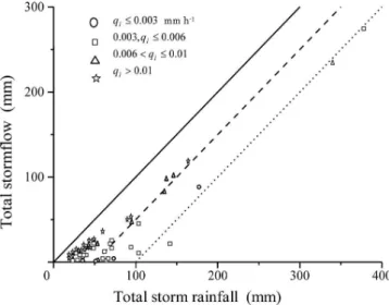
Fig. 1. Relationship of the total stormflow to the total storm rainfall
in KT in TEF.qi: runoff rate before the storm event. Solid,
bro-ken, and dotted lines indicateQ=R, Q=R−50, Q=R−100, respectively, whereR is the total storm rainfall andQis the total stormflow. After Tani and Abe (1987).
2 Hydraulic continuum from a review on site observations
2.1 Extension of the stormflow contribution area
Runoff discharge is generally distinguished into stormflow and baseflow by a recession gradient, and the stormflow re-sponses and their generation mechanisms are largely influ-enced by the magnitude of a storm. In general, when rain-fall begins, stormflow will generate from local wet zones and have very small volume. As rainfall increases, the contribu-tion area of stormflow extends with time (Hewlett and Hib-bert, 1968). However, when the cumulative rainfall becomes large enough, the contribution area may extend to almost the entire catchment. This tendency can be detected in the rela-tionship of stormflow volume per unit catchment area to the total rainfall volume of each storm event, which has been illustrated frequently as a means to understand the storm runoff characteristics in a catchment (Soil Conservation Ser-vice, 1972; Okamoto, 1978). Figure 1 shows an example of catchment Kitatani (KT) in the Tatsunokuchi-yama Experi-mental Forest (TEF), Okayama, Japan (Tani and Abe, 1987). When the amount of rainfall is small, stormflow is low be-cause most of the rainwater is stored in the soil layer by var-ious types of storage, such as canopy storage, litter storage, and absorption within small pores with low matric potential. The plots in Fig. 1 show clear control by the initial runoff rate as well as cumulative rainfall, suggesting the important effect of dryness before a storm event. The volume of storm-flow increases more quickly with rainfall when cumulative rainfall exceeds a threshold value.
After the cumulative rainfall exceeds the threshold volume in a large-scale storm, almost all of the additional rainwater tends to be allocated to stormflow (Tani, 1997). Therefore, we can imagine that the entire catchment area eventually con-tributes to stormflow production, even though some rainwa-ter may still be allocated to deep infiltration in catchments with geologies such as granite (Shimizu, 1980). However, the most important characteristic after the cumulative rainfall be-comes large enough during a large-magnitude storm is that the contribution area is spatially invariable. Although such large storms may be infrequent, they can provide very impor-tant information about stormflow responses and their mech-anisms. Two examples from hillslope observational studies are reviewed below.
2.2 Stormflow observations in catchments with fixed contribution areas
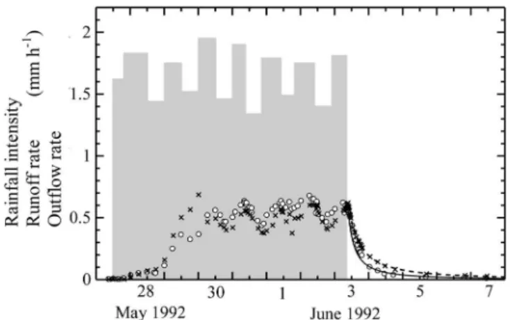
A valuable study of sprinkling experiments was conducted in the Oregon Coast Range, USA, to understand the storm-flow mechanism under the ground (Anderson et al., 1997; Montgomery et al., 1997; Ebel et al., 2007). The site labelled CB1 was a steep zero-order catchment (860 m2and 43◦) on Eocene volcaniclastic sandstone bedrock. Rainfall of a rela-tively weak intensity (average of 1.65 mm h−1)was supplied for a long duration (7 days), and all the water infiltrated into the soil. Two weirs (upper and lower) measured flow rates from both colluvium and fractured bedrock in the catchment, where the flow through the upper weir was separated from that through the lower weir, which was located 15 m down-stream. As shown in Fig. 2, the flow rates measured at the upper and lower weirs were roughly constant, equal to about one-third of the supplied rainwater intensity, after the suffi-cient rainfall was supplied. Both flow rates had a daily oscil-lation due to evapotranspiration and wind-induced variations in the rainfall intensity. The rainfall intensity with a large spa-tial distribution was manually measured twice daily, and the flow rate at each weir was measured by hand. Thus, temporal changes could not be recorded in detail (Ebel et al., 2007), and the results illustrated in Fig. 2 can be used only for a rough comparison because of the time lags. However, the re-sults indicated that during the 4-day period when the flow was nearly steady, the rainfall of 1.65 mm h−1was allocated to the averaged total flow rate of 1.1 mm h−1. Although deep infiltration constituted a leakage of 0.5 mm h−1(Anderson et al., 1997), the remaining rainwater contributed to stormflow responses, and the constant discharge rate suggested the tem-poral invariability of its contribution area.
Fig. 2. Sprinkled rainfall and runoff responses in CB1. Bar: rainfall; : runoff rate at the upper weir;×: runoff rate at the lower weir. The solid and broken lines are the outflow rates calculated by TANK using the functional relationship between storage and the outflow rate in Eq. (2) with apvalue of 0.3 andkvalues of 11 for the upper weir and 20 for the lower weir. Recreated from Fig. 3 of Anderson et al. (1997); courtesy of Dr. Suzanne Anderson.
weirs roughly followed, with a small delay, the daily oscil-lation of rainfall intensity during the nearly steady state, re-gardless of the limitations of the hand measurements. For the flow response to rainfall, Anderson et al. (1997) found the following processes through two kinds of tracer experiments. A high-speed subsurface flow from the fractured bedrock to the outlet through the colluvium was detected by bromide point injections into the saturated materials. Another exper-iment using sprinkler water labelled by deuterium showed plug flow without preferential flow for the vertical unsatu-rated water movement.
These tracer experiments strongly suggested that a com-bination of a vertical plug flow in the unsaturated zone and high-speed downslope flow in the saturated zone can produce rapid flow responses at the timescale of stormflow to daily rainfall oscillations. Note that although water must theoreti-cally move according to the gradient of hydraulic head, the unsaturated vertical flow and saturated downslope flow were
seemingly disconnected by remaining a dry portion of the soil
layer in the early stage of the experiment. This disconnec-tion was hydraulically resulted from a negligible small value of the unsaturated hydraulic conductivity in the dry portion compared to that in each of the wet zones near the surface above the wetting front and at the capillary fringe near the saturated zone. The flows were efficiently connected during the nearly steady-state stage after the entire soil layer had become sufficiently wet. Thus, we now defined this
substan-tively connected system as “hydraulic continuum” (called
HC in this paper). This experiment showed that a creation of HC connecting the unsaturated and saturated flows played an important role in quick flow responses. Approximations that neglect unsaturated flow have often been used for analysing water movement beneath the ground (Brutsaert, 2005), but
the results from CB1 suggest that such an approximation should be rejected here because it is not fixed whether the sat-urated or the unsatsat-urated flow has the larger effect on storm-flow responses. The important role of hydrologic or hydraulic connectivity in catchment processes has already been dis-cussed elsewhere (Michaelides and Chappell, 2009; Oldham et al., 2013), and HC, efficiently connecting the unsaturated and saturated flows, will be used as a key concept for the flow responses in this paper.
A similar runoff process was estimated from two small forested catchments, KT (17.3 ha) and MN (Minamitani of 22.6 ha, an adjacent catchment of KT), in TEF (Tani, 1997). The soil was a clay loam derived from the sedimentary rock. Although the soil was generally deep, the two catchments were both characterised by high stormflow volumes when most of the rainfall was allocated to the stormflow under wet conditions after the rainfall volume exceeded the threshold of cumulated rainfall, as shown in Fig. 1 for KT. For quick flow responses, the vertical water movement was not estimated as a preferential flow but as unsaturated flow through the soil matrix. Evidence was further derived from measurement of matric potential in the soil layer on a steep planar hillslope (500 m2 and 35◦) in MN. In the early stage of the storm, the dry portion within the soil, substantively disconnecting the water flow, gradually disappeared due to the downward development of a wetting front. Stormflow generation was enhanced after HC was created by the water-flow connec-tion in the entire hillslope. The matric potential near the soil surface had a clear positive relationship with the given rain-fall intensity, as predicted theoretically from Darcy’s law by Rubin and Steinhardt (1963), demonstrating the vertical wa-ter movement by the unsaturated flow through the soil matrix instead of the preferential flow (Tani, 1997).
In addition to this planar hillslope observation, another study in TEF showed that the groundwater level at 15 m depth in a steep zero-order catchment with very thick soil increased quickly in response to rainfall, similar to the storm-flow rate during wet conditions in an upper soil layer, al-though the level did not respond during dry soil conditions (Hosoda, 2008). Quick downslope water movement was not explicitly traced, as it was in CB1, but a quick stormflow re-sponse with volume comparable to that of rainfall frequently occurred without overland flow in these catchments. This re-sult suggested that these stormflow characteristics may be produced from HC similar to that in the CB1 catchment. Next we investigate the nature of HC using the model of a single tank with a drainage hole.
2.3 Characteristics of inflow/outflow transmission by a single tank with a drainage hole
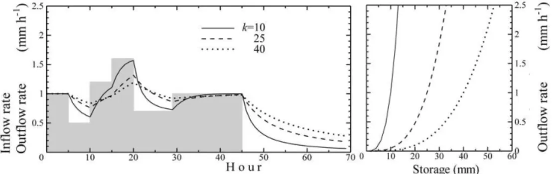
Fig. 3. Schematic example of outflow rates calculated by TANK in response to fluctuations in the inflow rate around the average of 1 mm h−1
and their recession limbs after the inflow stops (left panel). The functional relationships between storage and the outflow rate used in the calculations in the left panel are displayed in the right panel. The commonpvalue of 0.3 and the threekvalues described in the left panel were used for the TANK calculations.
1988), and the TOPMODEL (Beven and Kirkby, 1979). Although these models contain an algorithm for rainwa-ter allocation to stormflow and loss – the so-called separa-tion process of effective rainfall – stormflow responses may have a common characteristic represented by TANK. A gen-eral function for inflow/outflow waveform transmission by TANK can be written as
dVT
dt =i−o, (1)
whereVTis the TANK storage,iis the given inflow rate such as effective rainfall intensity, andois the outflow rate such as the stormflow rate (all per unit catchment area). Most runoff models have represented the relationship betweenoandV
for the stormflow components (Kimura, 1961; Kadoya and Fukushima, 1976) as
VT=kop, (2)
wherekandpare parameters. The inflow/outflow waveform transmission by TANK typically exhibits a “quasi-steady state” characteristic (called QSS in this paper). A QSS sys-tem is characterised by a dynamic equilibrium of storage such that the outflow fluctuates in response to a small change in inflow around an average rate. After the inflow in this sys-tem stops, outflow gradually decreases, but the same func-tional relationship between storage and the outflow rate as exists during dynamic equilibrium is kept in this recession stage (Meadows, 2008). This characteristic of a QSS system is derived strictly from the one-to-one relationship between storage and flow rate without hysteresis. Note that runoff re-sponses consisting of components with different timescales do not present the behaviour of a QSS as suggested from Sugawara’s tank model consisting of serially concatenated tanks. Therefore, catchment runoff responses are never char-acterised by QSS, but we can say that stormflow responses tend to represent this characteristic after the separation of ef-fective rainfall.
The quantitative properties of the QSS system are exam-ined further here. The water balance of Eq. (1) is transformed to
do
dt = i−o
dVT/do
. (3)
This equation implies that wheni=o,ois constant; when
i > o,oincreases; and wheni < o,odecreases. In addition, do/dtis controlled by dVT/do. Therefore, if the system is in a quasi-steady state, the increase/decrease rate of the outflow is simply controlled by the differential coefficient of storage with respect to outflow rate in a steady state.
The left panel in Fig. 3 is a schematic example showing the response of the outflow rate to a fluctuation in the inflow rate, the average of which is 1 mm h−1. The relationships between storage and outflow rate are represented by Eq. (2) and illus-trated in the right panel of Fig. 3. We used a commonpvalue of 0.3 and three differentkvalues of 10, 25, and 40 in Eq. (2) in consideration of the range of observed recession flows, as explained later in Sect. 2.4. The figure clearly shows the de-pendence of the increase/decrease rate of outflow on dVT/do, not only during the dynamic equilibrium in response to the cyclic fluctuations of inflow but also in the recession stage after its stop.
2.4 Application of TANK to observations
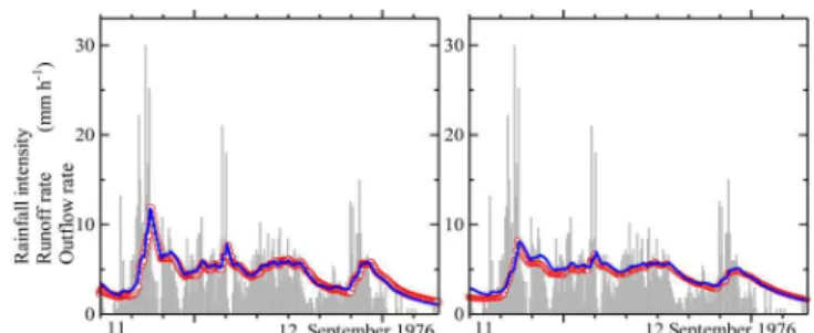
Fig. 4. Storm hydrographs, observed and simulated by TANK, in
re-sponse to a typhoon in September 1976 at KT (left) and MN (right) in TEF. Bar: 10 min rainfall intensity (displayed in mm h−1). Red circle: observed runoff rate. Blue line: simulated outflow rate. The lines were calculated by TANK using the functional relationship be-tween storage and the outflow rate given by Eq. (2) with a common
pvalue of 0.3 andkvalues of 25 for KT and 40 for MN.
for MN); thus we neglected the effect of the baseflow in-crease on the hydrograph during the event. Figure 4 plots the later stage of the entire event after the stormflow contribu-tion area might have extended to the entire catchments. The optimised value ofp for both catchments was 0.3, and the values ofkfor KT and MN were 25 and 40, respectively. Ex-tremely close agreement was obtained for each of the catch-ments, and the lower peaks and gentler recession limbs for MN vs. KT were accurately simulated by the difference ink
between them. This probably reflects thicker soil layers with gentler slopes in MN than KT, considering that there was a slightly larger annual evapotranspiration for MN than KT, as estimated from the 69 yr annual water balance there (Tani and Hosoda, 2012).
For CB1, the latter half of the sprinkler experiment was nearly in a steady state with a fixed contribution area, but the total of the flow rates fluctuated around 1.1 mm h−1, less than the rainfall rate because the constant loss rate remained continuously. It was difficult to evaluate the simulation re-sults by TANK in terms of runoff responses during the nearly steady state due to the manual measurements of rainfall in-tensity and runoff rates. The recession stage of runoff rate can be simulated only for each of the upper and lower weirs (Fig. 2). An optimised value ofpof 0.3 was also used here, and the optimised values ofkwere 11 and 20 for the upper and lower weirs, respectively. The values ofkwere slightly lower than those of TEF, but as compared with the calcula-tions represented in Fig. 3, the hydrographs for these catch-ments commonly have quick recession limbs with a small range of half-lives (roughly from several hours to one day) despite the large differences in catchment properties between them.
2.5 Stormflow responses for general cases
The accurate simulation results for TEF and CB1 shown above suggest that stormflow responses can be represented
by TANK, described by the storage and flow-rate relationship in Eq. (2), even though two flow mechanisms with differ-ent speeds were involved. A common characteristic of these examples is that the stormflow contribution area was ex-tended to the entire catchment and invariable after a sufficient amount of rainfall supply. This spatial invariability is impor-tant for a QSS system. Usual catchment runoff responses do not show this characteristic, as was mentioned in Sect. 2.3, and the plural contribution areas for stormflow and baseflow are both variable. Nonetheless, such good simulation results using Eq. (2) have been widely found in practical storm-flow analyses for flood management purposes in mountain-ous catchments in Japan when separation of effective rain-fall was conducted before hydrograph optimisation (Kimura, 1961; Sugiyama et al., 1997). Another example is an appli-cation of HYCYMODEL to seven small mountainous catch-ments (Tani et al., 2012). This model included TANK as part of the stormflow response. The application demonstrated that the gradients of stormflow recessions in catchments with dif-ferent land-use histories were similar, except for a catchment covered with bare land, where overland flow produced very quick recessions. A small range of stormflow recession gra-dients was also obtained from a comparison among about 90 mountainous catchments in Japan (Okamoto, 1978).
These TANK application results may suggest that, after the separation of effective rainfall, the stormflow contribu-tion area can be assumed approximately invariable for a short time during the storm event. Regardless of such empirically good applications, it is not clear why the stormflow responses can be simulated well by TANK with the parameter values of p andk shown in Eq. (2). Thep value of 0.6, reflect-ing the Mannreflect-ing equation for overland flow, was often rec-ommended (Kadoya and Fukushima, 1976; Fukushima and Suzuki, 1988), but this idea may be rejected because both saturated and unsaturated flows within the soil layer may in-volve the storage and flow-rate relationship instead of simple overland flow. Furthermore, it is also difficult to discern a physical meaning for thep value of 0.3 optimised for both CB1 and TEF. Strictly speaking, the exponential relationship in Eq. (2) is itself empirical and is difficult to explain on a physical basis.
3 Method of sensitivity analysis
3.1 Connection of observation and theory through the concept of hydraulic continuum
Although the flow mechanism in CB1 was found to be a com-bination of unsaturated flow within the soil matrix and quick saturated downslope flow, this conclusion was derived from only an individual result of tracer experiments. The observa-tion result in TEF suggested a similar mechanism but lacked tracer evidence. Overland flow was not a major source of stormflow in either observation, but a contribution from it cannot be rejected in general (Miyata et al., 2009; Gomi et al., 2010). Thus, we have to assume that such observations are site-specific and that an explanation for stormflow gen-eration by a different mechanism may be possible. General-isation of the mechanism determined from site observations may require theoretical consideration. This section quanti-fies the relationship between simple stormflow responses and their complex mechanisms based on hydraulic theory. For this purpose, sensitivities of these responses to topographic and soil properties are investigated, considering the hetero-geneity involved in the mechanisms. We use a methodology proposed by Tani (2008) for our sensitivity analysis because it was developed to theoretically connect flow responses from HC with water movement mechanisms in a sloping perme-able domain.
In Tani’s (2008) method, the runoff buffering potential (RBP) is defined as the difference between the water stor-age volumes within a domain in response to two steady-state outflow rates. Hence,
RBP≡ fb
Z
fa dV
dfdf =V (fa)−V (fb), (4)
wheref is the outflow rate per unit horizontal slope length, andV is the water storage volume within a permeable do-main. The meaning of RBP can be understood easily by com-paring the right and left panels in Fig. 3. As shown in that figure, the curve with a larger increase in storage in response to a given outflow-rate increase in the right panel produced a gentler fluctuation of the outflow rate in the left panel. There-fore, a larger RBP is an index for a gentler outflow-rate fluc-tuation. A larger RBP also contributes to a larger decrease in the peak outflow rate in usual non-steady natural condi-tions because of its smoothing effect, which is the reason for the name “runoff buffering potential”. When bothfbandfa are brought close tofm without limit, this integral form in Eq. (4) is converted to a differential form:
RBPIfm ≡ dV
df
fm, (5)
where RBPI is the index of RBP (newly introduced here and called RBPI) and fm is the averaged outflow rate around
whichf fluctuates. Figure 3 also shows that both the given inflow rate and the calculated outflow rate in the left panel fluctuate around fm=1 mm h−1, and each of the outflow-rate fluctuations shows its own delay in response to the RBPI value represented as the gradient of the curve (i.e. dV /df in the right panel).
For the recession stage from a storm event, substituting Eq. (5) into Eq. (3) gives the recession gradient atf as
df
dt =
−f
dV /df =
−f
RBPI. (6)
Hence the half-life (Th)atf is described as
Th= −ln(0.5)dV /df = −ln(0.5)RBPI. (7) This shows that the recession outflow rate from HC char-acterised by a QSS system is accurately reduced to a simple integral of the differential equation in Eq. (6). The left panel of Fig. 3 also shows an example of the recession in response to each of the RBPI values.
The purpose of this section on a sensitivity analysis is to connect simple stormflow responses and complex flow mech-anisms as already mentioned. We have to pay particular at-tention to a classic problem on hydrology that a good agree-ment of simulated and observed hydrographs cannot iden-tify the conditions assumed in the used runoff model (Betson and Ardis Jr., 1978). From this point of view, the creation of HC under QSS commonly characterised by both flow pro-cesses in a catchment with strong heterogeneities and a sim-ply idealised domain can contribute to our purpose. As noted in Sect. 2, the observational studies demonstrated that HC was created even in catchments with heterogeneous under-ground flow mechanisms consisting of slow unsaturated flow and quick downslope flow. Equation (5) for the RBPI and Eq. (6) for the outflow recession were strictly valid for HC created in every permeable domain based on the hydraulics. Accordingly, we can focus on determining what hydraulic conditions are required for producing the common character – that is, a quick inflow/outflow waveform transmission from HC under QSS – instead of optimising the model parameters for an individual hydrograph agreement. The conditions ob-tained from this theoretical sensitivity analysis may be more
generally approved to many complex catchments.
3.2 Sensitivity analysis for a sloping soil layer using a similarity framework
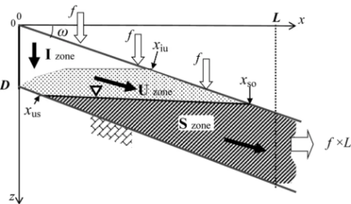
Fig. 5. Schematic of a sloping permeable domain with approximate
categorisation of the pressure head (I, U, and S zones). The horizon-tal distances involving the categorisation ofxiu,xus, andxsoare also
plotted.
key role in our sensitivity analysis specifying, with high gen-erality, the critical hydraulic conditions. However, so as not to disrupt the logical flow of this section, these are described in the appendices of this paper. The fundamental equations are introduced in Appendix A, and the main body of the text presents the key points of the sensitivity analysis.
Assume a steady state for the soil layer in response to rain-fall supply with a constant intensity, the range of which is less than the saturated hydraulic conductivityKs. The spatial distribution of pressure head within a soil layer can be cal-culated by the Richards equation (Eq. A1). Consider a soil layer under a steady state in response to a constant inten-sity of the rainfall first. When the rainfall is changed to a different constant intensity, this change in the surface bound-ary condition may be transmitted to the spatial distribution of pressure head in the whole soil layer governed by the lo-cal hydraulic head gradient according to the Richards equa-tion, and the outflow rate from the layer may be shifted to a new steady-state rate. Because the total volumetric water content integrated over the soil layer has a one-to-one rela-tionship with the outflow rate for both the new and old steady states, this layer will behave as HC under QSS, similar to TANK, whose flow responses are illustrated in the left panel of Fig. 3. Therefore, from the relationship of the total water storageV to the steady outflow rate per unit slope lengthfm, which is equal to the rainfall intensity because of the steady state, we can calculate the RBPI (Eq. 5) and the recession hydrograph (Eq. 6) for this soil layer. Thus, the sensitivity of the RBPI and recession characteristic to topographic and soil properties can be assessed through this calculation process. The macropore effect on water movement was considered in only the saturated zone as a hydraulic conductivity that is
εtimes larger thanKs according to a parameterisation pro-posed by Tani (2008) (Eqs. A14 and A15); this effect may not be present in an unsaturated zone due to a negative potential (Wang and Narashimhan, 1985; Nieber and Sidle, 2010).
Tani (2008) categorised the spatial distribution of the pressure-head value in a steady state within a soil layer on a steep slope, which is important for understanding the wa-ter flow in the layer described by the Richards equation. Three zones were approximately categorised (as shown in Fig. 5): the I zone with vertical unsaturated flow, the U zone with unsaturated downslope flow, and the S zone with satu-rated downslope flow. Regardless of the complex appearance of saturated–unsaturated flow, the pressure-head distribution was characterised simply by this hydraulic zoning. It is there-fore useful to understand the dependence of RBPI on slope properties. Tani (2008) also formulated indicators partition-ing the three zones. The indicators modified into dimension-less form for our similarity framework are described within Appendix B. It is important for generalisation that the cate-gorisation can provide a hydraulic background for both the vertical unsaturated flow and downslope saturated flow sug-gested from the on-site observations in CB1 and TEF because these two components may respectively reflect the I zone and the S zone with the U zone lying above.
To make our sensitivity analysis more general, a similar-ity framework was introduced using a small number of di-mensionless parameters (Eqs. B1 to B9). A steady-state out-flow rate per unit slope length,fm, equal to the rainfall in-tensity, was selected as a criterion for the nondimension-alisation. The similarity frameworks for the pressure-head distribution and RBPI are described in Appendices B and C, respectively. Six parameters were introduced. Three are soil physical properties:κ, the ratio of saturated hydraulic conductivityKs tofm;σ, the standard deviation of the log-transformed soil pore radius; andε, the parameterisation of the macropore effect in Ks. Two are topographical: ω, the slope angle, andλ, the ratio of the horizontal soil-layer length
dimensionless form, the calculations for them were respec-tively made in Eqs. (C3) and (C5).
Although the soil layers in our analysis in this section are based on a very simple assumption, they retain most of the core characteristics of the field observations in CB1 and TEF described in Sect. 2, which showed HC under QSS consist-ing of vertical unsaturated flow followconsist-ing Darcy’s law and downslope saturated flow with quick velocity. Spatial het-erogeneities in the hillslope are a major concern with respect to generality, and our parameterisation of the macropore ef-fect by the saturated hydraulic conductivity, represented by
ε, may not strictly reflect the pipe-like preferential pathways estimated by the tracer experiment in CB1. However, both of them can be regarded as similar from the hydraulic point of view because large-size pores commonly provide a high drainage capacity for the saturated downslope flow. Consid-ering such a heterogeneity influence, the next section about results of the sensitivity analysis presents the hydraulic con-ditions generally producing quick inflow/outflow waveform transmission and outflow recession from HC under QSS cre-ated within the sloping soil layer.
4 Results of sensitivity analysis
4.1 Sensitivity for RBPI
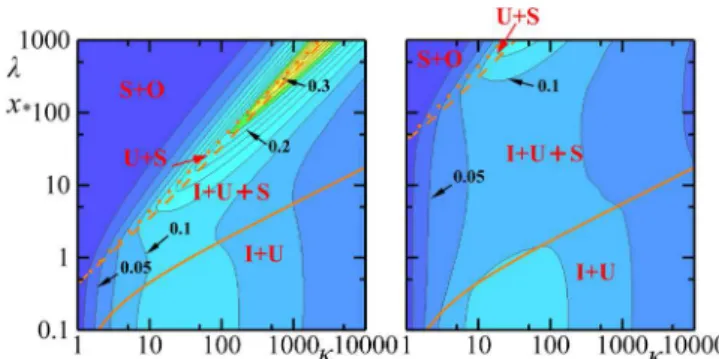
Figure 6 shows the sensitivity of RBPI∗ toκ and λ when
ω=30◦,δ=1, andσ=1.4. The left panel is forε=1 with-out any macropore effect, and the right panel is forε=100 with a large effect. The horizontal distances of indicators cat-egorising the pressure-head distribution, such asxiu∗,xus∗,
andxso∗in Eqs. (B10) to (B14), are plotted along the
ordi-nate axis for the horizontal distancex∗, also representing the layer lengthλ. This categorisation shows which of the I, U, and S zones compose the vertical profile at any horizontal pointx∗along the sloping soil layer. For example, there is no S zone in the vertical profile whenx∗<xus∗because only the
unsaturated flow is sufficiently responsible for a small rate of the downslope flow. The I zone exists whenx∗< xiu∗, and
saturation-excess overland flow is generated whenx∗> xso∗. In the left panel, large RBPI∗ values are shown along a stripe between thexus∗andxso∗lines. This means that RBPI∗
has a maximum value when the groundwater table is rising (the S zone is growing), but it rapidly decreases towards the upper-left area of the stripe (> xso∗)because the
saturation-excess overland flow extending upslope causes decreasing RBPI∗(=dV∗/df∗). Along the ridge of RBPI∗, its value de-creases withκbecause of the effect of the soil physical prop-erties: the volumetric water content in the unsaturated zone of a clayey soil with a smallκ(=Ks/fm)value is close to saturation, and the increase in the total water storageV in response to a groundwater table rise is small, resulting in a small increase in RBPI∗compared to that in a sandy soil with a smaller water content in its unsaturated zone. Note that this
Fig. 6. Contour plots of RBPI∗againstκandλforε=1 (left) and 100 (right). Orange solid, dashed, and dotted lines represent the hor-izontal distances for the end point of the I zone (xiu∗), the start point
of the S zone (xus∗), and the start point of the saturation-excess
overland flow (xso∗), respectively. The red letters indicate which
zones are included in the vertical profile at each horizontal point of the sloping soil layer (see Fig. 5).
tendency of a small V increase for a clayey soil has been usually represented by a small value of “effective porosity” in an approximation of the groundwater flow with neglecting the unsaturated flow process (Brutsaert, 2005). In the lower area with small x∗ (i.e. short slope length), RBPI∗ is con-trolled mainly by the vertical unsaturated flow because most of the soil layer is covered with the I zone.
In the right panel with a large macropore effect, RBPI∗ is generally lower than it is in the left panel. This occurs because of a smaller storage change derived from the large drainage capacity of the S zone due to the macropore ef-fect compared to that for the no-macropore efef-fect case in the left panel. Because a large macropore effect causes a quite thin S zone and the total downslope flow in the U and S zones remains close to the bottom of the soil layer, RBPI∗ is almost independent of the storage change in the U and S zones. Hence, most of the soil layer is covered with the I zone, where water moves vertically, and RBPI∗ is sensitive to only the storage change in the I zone as if the slope length were short. Within the I zone, the volumetric water content has the same value throughout the soil layer, which has an unsaturated hydraulic conductivity that is equal to the rain-fall intensity; thus the rainwater can be transmitted vertically by the gradient of the gravity force (not by the pressure-head gradient) as was theoretically demonstrated by Rubin and Steinhardt (1963). Therefore, RBPI∗ is controlled only by the vertical unsaturated flow in the I zone regardless of the horizontal soil-layer lengthλ. The distribution of RBPI∗ in the right panel clearly shows this tendency.
4.2 Sensitivity for recession outflow rate
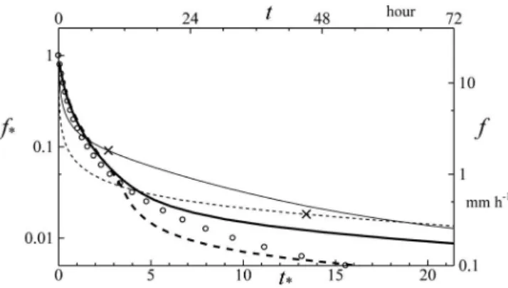
Fig. 7. Recession of the outflow rate from a sloping soil layer.
Di-mensionless scales are used for the bottom and left axes, and dimen-sional scales converted byfm=20 mm h−1are used for the top and
right axes. Thin solid line:λ=29.7 andε=1. Thin broken line:
λ=148.7 andε=1. Thick solid line:λ=29.7 andε=100. Thick broken line:λ=148.7 andε=100.×: the outflow rate in which the saturation-excess overland flow is generated at the downslope end of the domain. :calculated by the storage and outflow-rate relationship optimised for catchment KT, as also shown in Fig. 4.
criterion are also shown. The upper abscissa axis and right ordinate axis are scaled with the dimensional variables f
andt, whereas the lower and left axes are scaled with the dimensionless variables f∗ and t∗. The length scale l and the timescaleTf are converted to 67.24 cm by Eq. (B2) and 3.362 h by Eq. (C4), respectively, whenθs–θris assumed to be 0.1. The values of the other common parametersκ,δ,ω, andσ were 5.4, 1.49, 30◦, and 1.4, respectively. The
dimen-sional values of κ and δ are respectively converted to Ks of 0.003 cm s−1andD of 1 m. We used a parameter set of
λ=29.7 and 148.7 (their dimensional values are converted toL=20 m and 100 m, respectively) withε=1 and 100 for our recession-rate comparison. In addition to the calculation results, the simulation results using Eqs. (1) and (2) with pa-rametersp=0.3 andk=25 that were optimised for a storm event in catchment KT at TEF, as shown in Fig. 4, are also plotted for the dimensional scale.
For the calculations with no macropore effect (ε=1), saturation-excess overland flow was generated when the runoff rate exceeded the threshold indicated by the “×” mark in Fig. 7. The weight of the overland flow increased with the horizontal length of the sloping layer. In contrast, a high drainage capacity due to the macropore effect (ε=100) re-duced the rise in the water table and limited the occurrences of overland flow. When the macropore effect is large, the re-cession of the outflow rate depends little on the downslope flow in the U and S zones but is instead controlled mainly by the vertical water movement in the I zone. Both reces-sion outflow rates with the macropore effect forL=20 m and 100 m are similar to the recession of the runoff rate in KT in Fig. 7 regardless of a difference in the horizontal slope length, suggesting that the vertical water movement may play
an important role in producing the stormflow recession char-acteristics as estimated from the observations (Montgomery and Dietrich, 2002).
4.3 Summary of the sensitivity analysis
The sensitivity analysis showed that the RBPI defined in Eq. (5) and the outflow recession represented by Eq. (6), both produced from soil layers with HC under QSS, had the fol-lowing characteristics: the saturated downslope flow in the S zone and the saturation-excess overland flow had a large influence on RBPI when the macropore effect was not in-volved. This effect generally contributed to decreasing RBPI and reduced occurrences of overland flow by increasing the drainage capacity of downslope flow. Therefore, for a large macropore effect, RBPI was controlled mainly by the vertical unsaturated flow regardless of the slope length. A compari-son of the recession flow with an observed result suggested the important role of the macropore effect in the production of quick recession outflow from the soil layer without the oc-currence of saturation-excess overland flow. For the produc-tion of inflow/outflow waveform transmission from HC un-der QSS, we can thus conclude that the unsaturated and sat-urated flows were never isolated, considering the importance of their connection. Furthermore, the large drainage capac-ity of downslope flow played a key role in the confinement of HC inside the soil layer due to a reduction of saturation-excess overland flow.
5 Discussion
5.1 Development of large drainage capacity accompanied by soil-layer evolution
From the sensitivity analysis for a sloping soil layer, one of the key hydraulic conditions is a large drainage ca-pacity of the downslope flow. If the drainage caca-pacity is small, saturation-excess overland flow will be dominant in the stormflow generation process, as was also suggested by Freeze (1972). Considering this difference in the flow pro-cess, we now discuss why such a large drainage capacity can be found for catchments in active tectonic regions with large-magnitude storms. This “why-type” question for heterogene-ity was raised by McDonnell et al. (2007), and its simple an-swer may be obtained from “the evolution process of the soil layer” against the severe erosional forces that exist in such regions, as discussed below.
in other areas of a catchment because of water conver-gence (Tsukamoto et al., 1982). However, analyses of cos-mogenic nuclides have demonstrated that soil is constantly denuded, even along the ridge lines surrounding hollows in zero-order catchments (Heimsath et al., 1999), at speeds of about 0.1–1.0 mm yr−1 in Japan (Matsushi and Matsuzaki, 2010). These studies suggest that soil produced from weath-ered bedrock continually moves from ridges down to concave hollows by gravity, which is similar to water movement but at a much longer timescale. Soil creep and small landslides probably contribute to this soil movement, although further studies are necessary to clarify this process. Hence, we can estimate a dynamic cycle of soil evolution processes, includ-ing landslides, on a shorter timescale of 102 to 104yr in a zero-order catchment than on a timescale of the topographic evolution. Soil-layer evolution may begin after a landslide only when soil particles on a denuded bedrock surface over-come the strong erosional forces from tectonic activity and heavy storms (Iida, 1999).
Two kinds of preconditions are absolutely necessary for soil-layer evolution. Soil particles produced from the de-nuded surface of weathered bedrock are so easily eroded by heavy rainfall that support by vegetation roots plays a key role in the soil evolution (Shimokawa, 1984). When a small denuded area is created by a landslide, vegetation and soil recover from the edge of the area through seeds supplied along with soil particles from surrounding areas (Matsumoto et al., 1995). Observations of bare land located on a gran-ite mountain in Japan (Fukushima, 2006) suggested that in a widespread denuded landscape, also including ridgelines, the soil cannot be semi-eternally recovered. This is because the interplay between vegetation and soil fails because of a poor seed supply. The effect of vegetation roots on slope stability is quite important even for a thick soil layer because of the effects of both root penetration perpendicular to the sliding surface and three-dimensional root entanglement (Kitahara, 2010).
Saturation-excess and infiltration-excess overland flows certainly occur in gentle slope areas such as riparian zones (Gomi et al., 2010) and in local areas with a low surface per-meability (Miyata et al., 2009), respectively. The acceleration of surface erosion and landslide initiation by the overland flows should be considered in quantifying the role of storm-flow generation processes in active tectonic regions. The re-sults of the sensitivity analysis in Sect. 4 showed a main role of saturation-excess overland flow in stormflow when the drainage capacity is not efficient for downslope flow in the soil. Then, the safety factor of a sloping soil layer de-creases because the groundwater table rises to the ground surface (e.g. Sidle et al., 1985), accelerating landslide ini-tiation. Hence, the efficiency of drainage capacity is critical for the sustainability of soil-layer evolution, at least in steep hollows where water converges. Because the effect of ero-sional forces is consistent throughout the period of soil-layer evolution, it has to be accompanied by the development of an
efficient drainage system. Only a few studies have discussed
how such a system with a large drainage capacity might
de-velop (Tsukamoto and Ohta, 1988). It may be that the pro-duction of a soil block reinforced by a vegetation root sys-tem and the erosion of fine soil particles beneath the ground could progress simultaneously, resulting in increased hetero-geneities in the permeability of the soil layer.
From the viewpoint of the longer timescale of topo-graphic evolution, however, soil-layer evolution cannot con-tinue forever because the safety factor will decrease with the growth of the soil layer itself (Sidle et al., 1985) and with the increased elevation difference between the ridge-line and streambed caused by the uplifting of mountain body and the erosion of streambed (Montgomery and Brandon, 2002). The robustness of soil-layer evolution will eventually fail, and once a landslide occurs, the large amount of water stored within the soil will be released instantaneously, some-times causing fluidisation of the collapsed soil and debris flow (Takahashi, 1978). Conversely, as long as the soil layer continues to evolve without landslide occurrences, most of the rainwater will be confined within the soil layer during a storm, even one with a large magnitude. A large drainage capacity of the downslope flow plays a key role in this con-finement, which is necessary for continuous soil-layer evolu-tion, and ensures that simple and quick stormflow responses will be produced from HC under QSS created inside the soil layer. Thus, both the development of an efficient drainage system and reinforcement by a vegetation root system may be associated with the evolution of the soil layer.
5.2 A possible modelling strategy
stormflow component is represented by only a downslope-flow component (Ishihara and Takasao, 1964; Troch et al., 2003). The dependence of stormflow responses on unsatu-rated vertical flow has often been discussed from on-site ob-servations (Montgomery and Dietrich, 2002) and from theo-retical considerations (Tani, 1985a; Kosugi, 1999). As a re-sult, parameterisation of catchment properties must consider the historical evolution of the soil layer for distributed runoff models of active tectonic regions.
An additional insight into the evolution process provides another suggestion for predicting large-magnitude stormflow responses. As long as the stormflow is confined within the soil layer, as explained in Sect. 5.1, the characteristics of waveform transmission between the rainfall intensity and stormflow rate will be consistent for various storms with large magnitudes. Hence, this consistency may provide a use-ful clue to a prediction of stormflow responses in rare storm events never before observed because the validity of model predictions may be guaranteed except in the case of landslide occurrences.
Finally, in addition to these fundamental subjects, to bet-ter predict stormflow, more comparative studies are needed to identify which properties stormflow responses are dependent on. Although the dependences deductively introduced from the surface topography as usually used in distributed runoff models might be often regarded doubtful by on-site observa-tions in active tectonic regions (Montgomery and Dietrich, 2002; Weiler et al., 2006; McDonnell et al., 2007), only a few studies have focused on intercomparison (Negley and Eshleman, 2006; Uchida et al., 2006; Tani et al., 2012). Since many observations of stormflow responses have already been obtained, a higher priority should be given to an inductive detection of the dependences on catchment properties by the intercomparison of these data to apply the results to runoff-model parameterisations.
6 Conclusions
Many distributed runoff models have been developed, but it is still difficult to predict stormflow responses in catchments with no observational data used for the parameter calibra-tion and to predict responses to storms of larger magnitude than have ever been observed even in catchments with obser-vational data. To address such problems, this paper proposes the simple idea that stormflow responses reflect the soil-layer evolution process.
This idea was originally based on individual observational results on stormflow responses and their mechanisms, and the review suggested that HC under QSS played a key role in the production of these responses. The following new findings were obtained from this concept. (1) Stormflow re-sponses were simply produced from HC under QSS when the stormflow-contribution area was spatially invariable due to the sufficient amount of rainfall supply. (2) The sensitivities
of stormflow response for a sloping soil layer to the soil and topographic properties were examined using a new similarity framework with six dimensionless parameters when a steady-state flow rate was given as a criterion. (3) The examination showed that a large drainage capacity played a key role in the quick inflow/outflow transmission, and contributed to a reduction of saturation-excess overland flow and a confine-ment of water flow within the soil layer. (4) Discussion on the soil-layer evolution suggested that this confinement was needed for the evolution against strong erosional forces in active tectonic regions with large-magnitude storms.
On the basis of these findings, we have proposed two strategies for stormflow prediction: a parameterisation of catchment properties in consideration of the historical soil-layer evolution, and comparative hydrology for inductively evaluating dependences of stormflow responses on catch-ment properties. These ideas presented in this paper can therefore provide a clue for improving a prediction of storm-flow responses by distributed runoff models from the catch-ment properties. As a result, because complex catchcatch-ment properties and simple stormflow responses were created by a long-term soil-evolution process, the development of dis-tributed runoff models should focus their parameterisation strategies on the underground structure rather than the sur-face soil topography. This concept may impose a paradigm shift in the prediction of stormflow responses in active tec-tonic regions.
Appendix A
Fundamental equations for sensitivity analysis
Like Tani (2008), we also assess a sloping soil layer with constant depth and homogeneous hydraulic properties using a two-dimensional form of the Richards equation. The origin is placed at the upslope end of the surface of the soil layer, and thex axis andzaxis are positive in the horizontal and downward directions, respectively (Fig. 5). For our calcula-tion, we use the upslope portion of a semi-infinite soil layer with horizontal lengthLand vertical depthDto avoid the lo-cal influences of specific boundary conditions such as seep-age faces. Because only a steady-state response to rainfall with a constant intensity is analysed here, the fundamental equation is given as
∂ ∂x
K∂ψ ∂x
+ ∂
∂z
K
∂ψ
∂z −1
=0, (A1) whereKis the hydraulic conductivity andψis the pressure head.
As the surface boundary condition, rainfall with a con-stant intensity (equal to the outflow rate per unit slope length
boundary condition along the slope surface is written as
qz=f whenψ <0 atz=xtanω, x≥0, (A2) whereωis the slope angle. Whenψreaches zero at the sur-face, a constant pressure condition (ψ=0) is imposed to saturation-excess overland flow. For the other boundary con-ditions, we assume that no water flow occurs along the bot-tom of the permeable soil layer and across the upslope end. Accordingly,
qz=0 atz=xtanω+D, x≥0, (A3)
qx=0 atx=0,0≤z≤D. (A4) Tani (2008) proposed an approximation for the steady-state distribution of pressure head based on the Dupuit– Forchheimer assumption (Beven, 1981) and confirmed its agreement with solutions by the Richards equation for a steep sloping soil layer. We also use this approximation because it can aid in understanding of the structure of the flow com-ponents. Three zones can be categorised as shown in Fig. 5: the I zone for the vertical unsaturated flow starts at x=0 but ends atx=xiu, after which the U zone for the downs-lope unsaturated flow grows up to the soil-layer surface. The S zone for the downslope saturated flow starts atxus, where the unsaturated flow rate within the U zone reaches the lim-itation. Saturation-excess overland flow starts atxsobecause the saturated downslope rate finally reaches the maximum. The indicatorsxiu,xus, andxsofor the categorisation can be calculated from the approximation and their dimensionless forms will be described later in Appendix B.
For soil physical properties controlling water retention and permeability, Kosugi’s (1996, 1997a, b) equations derived from log-normal soil pore distributions are used:
θ=(θs−θr)Se+θr
=(θs−θr)Q
ln(ψ/ψ
m)
σ
+θrforψ <0, (A5)
θ=θsforψ≥0, (A6)
K0=KsK∗. (A7)
Hereθis the volumetric water content;Seis the effective saturation;θsandθrare the saturated and residual volumetric water contents, respectively;ψmis the median pressure head corresponding to the median pore radius;σ is the standard deviation of the log-transformed soil pore radius (σ >0), which characterises the width of the pore-size distribution;
Qis the complementary normal distribution function,
Q(y)=(2π )−0.5
∞
Z
y exp
−u2
2
du; (A8)
K0is the hydraulic conductivity given by Kosugi’s equation, which is distinguished fromKbecause of the involvement of
the macropore effect described later; andK∗ is the relative unsaturated hydraulic conductivity, defined as
K∗=
Q
ln(ψ/ψ
m)
σ
1/2
×
Q
ln(ψ/ψ
m)
σ +σ
2
forψ <0 (A9)
K∗=1 forψ≥0. (A10)
Therefore, the relationships of volumetric water content and unsaturated hydraulic conductivity to pressure head de-scribed in above equations are represented by parameters in-cludingθs,θr,Ks,ψm, andσ. This means that the effects of soil physical properties on the hydraulics of a sloping soil layer can be assessed by a sensitivity analysis of these five parameters. However, this procedure may still be too tangled to extract the essence of each effect, making a simpler param-eter set desirable. First,θs andθrcan be removed using the effective saturation,Se, because of their linear contribution, and the retention and hydraulic properties can be written in terms ofKs,ψm, andσ. In addition, because the saturated hydraulic conductivityKsmay be dependent on the soil pore distribution, Ks andψm can be connected. Kosugi (1997a) proposed the following functional relationship based on the proportional relationship ofKsto the square of the arithmetic mean of pore radiusra.
Ks=Ara2=Arm2exp(σ2). (A11) Here,rmis the median pore radius andAis a proportional-ity constant. The relationship of capillary rise to pore radius is expressed as
ψ= −2γcosη
ρgr , (A12)
whereγ is the surface tension between the water and air,
η is the contact angle, ρ is the density of water, and g is the acceleration due to gravity. Substituting Eq. (A12) into Eq. (A11) yields
Ks=A
2γcosη
ρg
2 1
ψ2 a
= B
ψ2 a
=Bexp(σ 2)
ψ2 m
, (A13)
where ψa is the pressure head corresponding to ra. Kosugi (1997b) estimated the value of B [=A{(2γcosη)/(ρg)}2] as a constant value of 100.4cm3s−1 from a data set of soil hydraulic properties (Mashimo, 1960). As the parameter representing soil water retention, it is better to selectψathanψmbecauseKsis not related toσ, onlyψa. Hence, the soil physical properties can be represented by only two parameters.
As macropores play an important role in the hydraulics in our soil layer, their effect was parameterised here using a method proposed by Tani (2008):
K=K0 forψ <0, (A14)
whereε represents an empirical parameter for the macrop-ore effect. This parameterisation assumes that the macropmacrop-ore effect functions only within the saturated zone.
Appendix B
Similarity framework of the pressure-head distribution
A method using a similarity framework has been often ap-plied to runoff processes to generalise an assessment of the effects of catchment properties (Takagi and Matsubayashi, 1979; Harman and Sivapalan, 2009). We also introduce such a method to assess the dependence of RBPI on the proper-ties of slope topography and soil physics. Because RBPI is defined in Eq. (5) by the increase/decrease inV in response to a small increase/decrease in the outflow ratef around the averagefm,fmwas selected as the standard for our dimen-sionless form. The saturated hydraulic conductivityKs was made dimensionless as
κ=Ks fm
. (B1)
The dimensionless ratio between the depth of the soil layer and a parameter with the dimension of length rep-resenting the soil water retention characteristic curve has often been used for a similarity framework of saturated– unsaturated flow (Verma and Brutsaert, 1970; Tani, 1982, 1985a, b; Suzuki, 1984) because this ratio is a key controller of the relative importance of capillaries in the vertical dimen-sion of the permeable domain (Brutsaert, 2005). Becausefm is used as the standard in our analysis, the parameterl was selected for the length scale in reference to the relationship betweenKs andψain Eq. (A13) with the empiricalBvalue of 100.4(Kosugi, 1997b)
l=100.2/pfm. (B2) The parameterψain Eq. (A13) is made dimensionless by substituting Eqs. (B1) and (B2) into Eq. (A13), yielding
ψa∗=ψa/ l= −
p
1/κ. (B3)
The soil physical properties in our similarity framework are represented by only two dimensionless parameters,κand
σ.
The rainfall intensity (=outflow rate per unit slope length because of steady state)f, pressure headψ, horizontal axis
x, vertical axisz, horizontal soil-layer lengthL, and depthD
of the soil layer are made dimensionless as
f∗=f/fm, (B4)
ψ∗=ψ/ l, (B5)
x∗=x/ l, (B6)
z∗=z/ l, (B7)
λ=L/ l, (B8)
δ=D/ l. (B9)
When analysing the spatial distribution of pressure head in this similarity framework using six dimensionless param-eters –ω,λ,δ,κ,σ, andε– we can generally make an in-tercomparison of hydraulic characteristics within soil layers with various topographic and soil properties in a steady state with a flow rate offmas a criterion.
Indicators of the flow categorisation mentioned in Ap-pendix A and illustrated in Fig. 5 can be calculated from the relationship of vertical pressure-head distribution to the downslope flow rate at a horizontal distance (Tani, 2008) because a hydrostatic distribution based on the Dupuit– Forchheimer assumption is applied in our approximation. The dimensionless forms are described here as
xiu∗=
ψf∗+δcos2ω Z
ψf∗
K∗dψ∗κtanω
f∗ forα <1 (B10)
xiu∗=
0
Z
ψf∗
K∗dψ∗ +ε(δcos2ω+ψf∗)
κtanω f∗
forα≥1, (B11)
xus∗= 0
Z
−δcos2ω
K∗dψ∗ κtanω
f∗ forα <1, (B12)
xus∗= 0
Z
ψf∗
K∗dψ∗κtanω
f∗ forα≥1, (B13)
xso∗=
δεκsinωcosω
f∗ , (B14)
where the relative hydraulic conductivityK∗is calculated as follows by substituting Eq. (B3) into Eq. (A9):
K∗=
Q
ln(
−ψ∗√κ)
σ −
σ
2
1/2
×
Q
ln(
−ψ∗√κ)
σ +
σ
2
2
. (B15)
The pressure headψf∗included in the above equations rep-resents the dimensionless form ofψf, a constant pressure-head value in response tof in the I zone where the vertical flow is governed by only the gradient of gravity force (Ru-bin and Steinhardt, 1963). This relationship can be written in dimensional form as
K(ψf)=f. (B16)
Hence,ψf∗is inversely calculated by
K∗(ψf∗)=f∗/κ. (B17)
The pressure head in the I zone is
A dimensionless numberαcontrolling the structure of cate-gorisation within a soil layer is defined as
α= −δcos
2ω
ψf∗
. (B19)
In the U and S zones, a hydrostatic distribution based on the Dupuit–Forchheimer assumption is applied for a vertical pro-file as
ψ∗=ψb∗−(δ−z∗)cos2ω−x∗sinωcosω, (B20)
whereψb∗is the pressure head at the bottom of the soil layer. The value ofψb∗is inversely calculated from the downslope flow rate across the vertical soil-layer profile at a horizontal distance ofx∗. This flow rate can be obtained by integrat-ing the supplied vertical flow ratef∗ from the upslope end (x∗=0) tox∗because the system is in a steady state. The fol-lowing equations can be used for the calculation according to the categorisation of the pressure-head distribution described in Eqs. (B10) to (B14):
ψb∗ Z
ψf
∗
K∗dψ∗= f∗x∗
κtanω forx∗≤xiu∗andα <1,
orx∗≤xus∗andα≥1, (B21)
ψb∗ Z
ψb∗−δcos2ω
K∗dψ∗= f∗x∗
κtanω forxiu∗< x∗≤xus∗
andα <1, (B22)
0
Z
ψf
∗
K∗dψ∗+εψb∗=
f∗x∗
κtanω forxus∗< x∗≤xiu∗
andα≥1, (B23)
0
Z
ψb∗−δcos2ω
K∗dψ∗+εψb∗=
f∗x∗
κtanωforxus∗< x∗≤xso∗
andα <1,
orxiu∗< x∗≤xso∗andα≥1. (B24)
Appendix C
Similarity framework of the index of runoff buffering potential (RBPI)
To assess the RBPI for the sloping soil layer, the water stor-age volume per unit drainstor-age areaV is represented as the total volumetric water contentθper unit of horizontal length integrated over the whole soil layer:
V = 1 L
L
Z
0
xtanω+D
Z
xtanω
θdzdx. (C1)
For our nondimensionalisation described in Appendix B, the dimensionless storage volumeV∗is obtained as
V∗= V−Dθr l(θs−θr)=
Rλ
0
Rx∗tanω+δ
x∗tanω Sedz∗dx∗
λ . (C2)
The RBPI forfm in Eq. (5) is made dimensionless into RBPI∗for the unity as
RBPI∗f∗=1≡
dV∗
df∗ f∗=1 =
1
Tf
dV
df fm =
1
Tf
RBPIfm, (C3) whereTfis the timescale for the nondimensionalisation de-rived by submitting Eqs. (B4) and (C2) into Eq. (C3):
Tf=
l(θs−θr)
fm
. (C4)
This scale is the time necessary for filling the effective pores in a standard soil depth oflwith a standard flow rate of
fm. Equation (6) representing the recession gradient is made dimensionless as
df∗
dt∗ =
−f∗
dV∗/df∗=
−f∗
RBPI∗, (C5)
wheret∗is the dimensionless time defined as
t∗=t /Tf. (C6)
The recession flow rate from the starting rate of f∗=1 (f =fm in the dimensional form) can be obtained by the numerical integral using Eq. (C5).
Acknowledgements. I express my appreciation to Suzanne