www.biogeosciences.net/8/3025/2011/ doi:10.5194/bg-8-3025-2011
© Author(s) 2011. CC Attribution 3.0 License.
Biogeosciences
Towards accounting for dissolved iron speciation in global
ocean models
A. Tagliabue1,2,3and C. V¨olker4
1Laboratoire des Sciences du Climat et de l’Environnement, IPSL-CEA-CNRS-UVSQ Orme des Merisiers, 91198, Gif sur Yvette, France
2Southern Ocean Carbon and Climate Observatory, Council for Scientific and Industrial Research (CSIR), P.O. Box 320, Stellenbosch, 7599, South Africa
3Department of Oceanography, University of Cape Town, 7701, Cape Town, South Africa
4Alfred Wegener Institute for Polar and Marine Research, Am Handelshafen 12, 27570, Bremerhaven, Germany Received: 9 February 2011 – Published in Biogeosciences Discuss.: 16 March 2011
Revised: 1 September 2011 – Accepted: 4 October 2011 – Published: 31 October 2011
Abstract. The trace metal iron (Fe) is now routinely in-cluded in state-of-the-art ocean general circulation and bio-geochemistry models (OGCBMs) because of its key role as a limiting nutrient in regions of the world ocean important for carbon cycling and air-sea CO2exchange. However, the complexities of the seawater Fe cycle, which impact its spe-ciation and bioavailability, are simplified in such OGCBMs due to gaps in understanding and to avoid high computational costs. In a similar fashion to inorganic carbon speciation, we outline a means by which the complex speciation of Fe can be included in global OGCBMs in a reasonably cost-effective manner. We construct an Fe speciation model based on hy-pothesised relationships between rate constants and environ-mental variables (temperature, light, oxygen, pH, salinity) and assumptions regarding the binding strengths of Fe com-plexing organic ligands and test hypotheses regarding their distributions. As a result, we find that the global distribu-tion of different Fe species is tightly controlled by spatio-temporal environmental variability and the distribution of Fe binding ligands. Impacts on bioavailable Fe are highly sensi-tive to assumptions regarding which Fe species are bioavail-able and how those species vary in space and time. When forced by representations of future ocean circulation and cli-mate we find large changes to the speciation of Fe governed by pH mediated changes to redox kinetics. We speculate that these changes may exert selective pressure on phytoplank-ton Fe uptake strategies in the future ocean. In future work, more information on the sources and sinks of ocean Fe lig-ands, their bioavailability, the cycling of colloidal Fe species and kinetics of Fe-surface coordination reactions would be
Correspondence to:A. Tagliabue ([email protected])
invaluable. We hope our modeling approach can provide a means by which new observations of Fe speciation can be tested against hypotheses of the processes present in govern-ing the ocean Fe cycle in an integrated sense
1 Introduction
The role of the micronutrient iron (Fe) in governing phy-toplankton growth and primary production in large parts of the ocean is now well established (e.g., Boyd et al., 2007). One Fe-limited region of particular interest is the South-ern Ocean, which plays an important role in govSouth-erning air-sea CO2 fluxes (Takahashi et al., 2009) and is predicted to be impacted heavily by climate change (e.g., Sarmiento et al., 2004). Accordingly, most current generation three-dimensional global Ocean General Circulation and Biogeo-chemistry Models (OGCBMs) that seek to explore the con-trols upon the cycling of carbon and other nutrients, or the response of the ocean system to climate change typically all include Fe as a limiting nutrient for phytoplankton (e.g., Au-mont and Bopp, 2006; Moore and Braucher, 2008; Galbraith et al., 2010). However, the cycle of Fe in seawater is highly complex, with nominally “dissolved” Fe (dFe) able to exist as many different species, not all bioavailable to phytoplank-ton (e.g., Hutchins et al., 1999; Maldonado et al., 2006).
more organic ligands (Wu et al., 2001). Using electrochemi-cal techniques it has been shown that over large parts of the world ocean>99 % of dFe is actually complexed to organic ligands of typically unknown provenance (e.g., Gledhill and van den Berg, 1994; Van den Berg, 1995; Rue and Bruland, 1995; Wu and Luther, 1995; Boye et al., 2003; 2006). This is important as it prevents the precipitation/scavenging of free inorganic Fe(III) to solid forms, which are effectively lost from the dissolved pool and bioavailable Fe species. Fe lig-ands thus effectively increase both the solubility and resi-dence time of dFe in the ocean, as well as exerting a control on its bioavailability.
It has been shown that phytoplankton can access organi-cally bound Fe (e.g. Maldonado and Price, 1999), but not all forms of complexed Fe are equally bioavailable to differ-ent groups of phytoplankton (Hutchins et al. 1999). Mech-anisms for the uptake of organically bound Fe typically in-volves the reduction of the organically bound Fe by either specific reductases at the cell surface (Maldonado and Price 2001; Salmon et al., 2006; Maldonado et al., 2006), which is a mechanism well known from terrestrial plants (Moog and Br¨uggemann, 1994), or by excretion of reactive oxy-gen species (Shaked et al., 2005). Due to the diffusive loss of reduced Fe away from the cell, each of these mecha-nisms inevitably leads to some loss of Fe (V¨olker and Wolf-Gladrow 1999). Alternatively, phytoplankton can assimilate organically complexed Fe via specific uptake mechanisms (Boukhalfa and Price, 2002), which do not make the whole Fe pool bioavailable. All these mechanisms to access or-ganically complexed Fe seem costly compared to the up-take of inorganic Fe species, which can be assimilated rel-atively straightforwardly (Hudson and Morel 1990; Morel et al., 2008) and means inorganic Fe can be thought to be the most bioavailable Fe fraction. Organically bound, as well as inorganic colloidal, Fe(III) can also be photoreduced in the presence of light to produce Fe(II) (e.g., Barbeau et al., 2003; Croot et al., 2008). As such, the speciation, residence time and bioavailability of Fe in the ocean depend on a suite of processes that are themselves highly sensitive to the envi-ronmental conditions of the ocean.
In the context of its complex speciation and cycling, dFe is treated very simply in “state-of-the-art” OGCBMs, with only a single dFe pool represented and ligand complexation accounted for assuming a single ligand of uniform concen-tration (e.g., Parekh et al., 2004; Aumont and Bopp, 2006; Moore and Braucher, 2008; Galbraith et al., 2010). Spatio-temporal variability in Fe speciation, cycling and bioavail-ability is therefore ignored. Alongside the lack of constraints from observations, this is mostly due to the prohibitive com-putational cost of simulating rapid Fe cycle reactions at the global scale. Three-dimensional regional models have mod-eled the Fe cycle in a prognostic fashion for Fe-limited wa-ters and noted the potential role of environmental variability in governing the supply of Fe to phytoplankton (Tagliabue and Arrigo, 2006). Similar models have also been employed
in a one-dimensional framework at time series sites in the subtropical and tropical Atlantic Ocean (Weber et al., 2005, 2007; Ye et al., 2009). Recently, Tagliabue et al. (2009) in-cluded the first order impact of light and temperature on Fe speciation in a 3-D OGCBM and suggested that the role of environmental variability in Fe speciation could be important in governing the residence time and bioavailability of dFe in the ocean.
Over the coming century, the ocean is predicted to un-dergo a great deal of environmental change, especially the Fe-limited Southern Ocean. It is likely that temperatures will rise, stratification will increase, light levels will increase, pH will fall (due to the uptake of anthropogenic CO2)and reduced sea ice will extend the growing season. All of these changes might impact upon the speciation of Fe and some experimental evidence from mesocosm experiments in-deed suggests “acidification” induces changes to Fe(II) lev-els (Breitbarth et al., 2010), while laboratory experiments us-ing synthetic ligands lead to modifications to Fe bioavailabil-ity that depend upon the type of chelator considered (Shi et al., 2010). As it stands, even including the first order im-pact of light and temperature on the marine Fe cycle (as per Tagliabue et al., 2009) will not resolve the matrix of paral-lel changes resulting from climate change that will impact Fe cycle rate processes (e.g., oxidation rates, photoreduction rates), the dFe concentration itself and the concentration of ligands. To address these questions we require a tool that can resolve the speciation of Fe in a semi-prognostic manner at the global scale in a ‘cost effective’ manner. In this study, we outline a new approach that permits the ‘semi-prognostic’ modeling of Fe speciation at the global scale using an analyt-ical approach similar to that typanalyt-ically employed for inorganic carbon speciation. We then use this model to speculate how Fe speciation might respond to the climate associated with an atmospheric CO2concentration of∼1000 ppm as an illustra-tion of how our Fe speciaillustra-tion model can be applied.
2 Theoretical framework
OGCBMs that seek to compute inorganic carbon speciation for air-sea CO2exchange or pH calculations.
The full equations of the dFe model used here and their sensitivity to various parameter modifications are presented in Tagliabue and Arrigo (2006) and Tagliabue et al. (2009). The state variables of the model are the free concentrations of Fe(II) (Fe(II)′), Fe(III) (Fe(III)′), Fe(III) bound to the weak non-bioavailable ligand (FeLW)and the strong bioavailable ligand (FeLS), solid Fe(III) (Fep, which could be thought to include colloidal Fe(III)), the total dFe concentration (FeT), the uncomplexed weak (LW)and strong (LS)ligands and the total concentration of LW(LWT)and LS(LST). We disregard here complexation of Fe(II) by organic ligands. Ferrous iron complexes have been suggested to be possibly responsible for the long residence time of Fe(II) in the SOIREE iron fer-tilization experiment (Croot et al., 2001), but have only been demonstrated in riverine or coastal waters with high fulvic acid concentrations (Voelker and Sulzberger, 1996 and Rose and Waite, 2003). However, such Fe(II) specific ligands may be difficult to identify using current techniques when they are at low abundance (e.g., Croot et al., 2007, 2008). Rate con-stants required by the model are the oxidation of Fe(II)′(kox, which is a function of temperature, pH, salinity and oxygen concentrations), photoreduction of FeLW(kphW, which is a function of irradiance as per Tagliabue et al., 2009) and FeLS (kphS), the formation of FeLW(klW)and FeLS(klS), the dis-sociation of FeLW (kbW)and FeLS (kbS), the precipitation of Fe(III)′to FeP(kpcp)and the remineralization of FeP(kr). Re-arranging the differential equations for the Fe species re-sults in the following four governing equations:
0=klWFe(III)′LW−kbWFeLW−kphWFeLW (1) 0=klSFe(III)′LS−kbSFeLS−kphSFeLS (2) 0=kphWFeLW+kphSFeLS−koxFe(II)′ (3)
0=kpcpFe(III)′−krFeP (4)
Additional constraints are that the concentrations of FeT, LWTand LSTmust be conserved over the fast timescale: FeT=Fe(III)′+Fe(II)′+FeLW+FeLS+FeP (5)
LWT=FeLW+LW (6)
LST=FeLS+LS (7)
In order to solve the model analytically first requires a rear-rangement of Eqs. (3 and 4) to yield:
Fe(II)′=kphW kox
FeLW+ kphS
kox
FeLS (8)
and FeP=
kpcp kr
Fe(III)′. (9)
These equations are then inserted into Eq. (5) to result in: FeT=aFe(III)′+bFeLW+cFeLS (10) where a = 1 +kpcp/kr, b = 1 +kphW/kox, and c = 1+kphS/kox. From Eqs. (6 and 7) it follows that the free ligand concentra-tions are:
LW=LWT−FeLW (11)
LS=LST−FeLS. (12)
Equation (12) can now be used in combination with Eq. (2) to produce:
0=klSFe(III)′(LST−FeLS)−(kbS+kphS)FeLS (13) and solved for FeLS:
FeLS=
Fe(III)′L ST KS+Fe(III)′
(14) where KS= (kbS+kphS)/klS. Equation (14) is then combined with Eq. (10) to solve for the concentration of FeLW:
FeLW=klWFe(III)′
LWT−FebT+ aFe(III)′
b +
cFe(III)′ b
LST
KS+Fe(III)′
−(kbW+kphW)
FeT b −
aFe(III)′
b −
cFe(III)′ b
LST
KS+Fe(III)′
. (15)
Inserting Eq. (15) into Eq. (1) permits us to obtain an equa-tion for Fe(III)′which, after simplification and sorting into powers of Fe(III)′, yields a third order polynomial solution for the concentration of Fe(III)′:
0=(Fe(III)′)3+bLWT
a +
cLST
a +KS+KS− FeT
a
(Fe(III)′)2 +KSbLaWT+KWcLaST+KWKS−(KW+KS)FeaT
Fe(III)′
−KWKSFeaT
(16)
where KW = (kbW+kphW)/klW. Equation (16) can be solved analytically or iteratively and has three solutions, but only one is positive and thus a realizable Fe(III)′ concentration. Therefore by first solving Eq. (16) for the Fe(III)′ concentra-tion, one can then proceed to solve for the FePconcentration (Eq. 9), FeLS concentration (Eq. 14), FeLW concentration (Eq. 15), and finally the Fe(II)′ concentration (Eq. 8). Thus
for a given set of rate constants, which are either fixed or vary as a function of environmental variables, and the con-centrations of FeT, LWT, LST, the procedure outlined above analytically solves for the concentrations of the 5 Fe species (Fe(II)′, Fe(III)′, FeLW, FeLS, and FeP)at considerably less computational expense than a prognostic solution.
3 Inclusion in an OGCBM
3.1 Modeling framework and experiments
2006), since this model has been widely used for ocean bio-geochemistry and climate applications, including some ad-dressing Fe speciation (e.g., Tagliabue et al., 2009). Firstly, the analytical solution of Eq. (16) was solved iteratively in each grid cell of the model at each time step to yield the Fe(III)′ concentration. From this, the concentrations of all other Fe species can then be computed. The analytical solu-tion uses properties that are either provided by the PISCES model (FeT, LWT, LST)or computed in each grid cell and at each time step from variables simulated by the PISCES model (kox,kphW,kphS,klW,klS,kbW,kbS,kpcpandkr). For example,koxwill vary in space and time as a function of the temperature, pH, oxygen concentration, and salinity, follow-ing the equation of Santana-Casiano et al. (2005), whilekphW andkphSwill vary with depth and season following available radiation each particular model grid cell (all other rate con-stants are initially fixed in space and time). The total dFe pool is also modified each time step by phytoplankton up-take and remineralisation and all other source – sink terms for dFe traditionally included in the PISCES model (see: Au-mont and Bopp, 2006 for a full list of Fe equations). We find that the calculated FeT computed from the sum of all species calculated analytically is generally less than±1 % in error relative to the dFe tracer prognostically simulated by PISCES (which is an input to the speciation solution) and only reaches a maximum of±5 % error in a few isolated grid cells (below 75 m and 150 m the error is less than±1 % and ±0.1 %, respectively). This demonstrates that our procedure has an acceptable error in calculating Fe speciation, espe-cially considering the global nature of its application and the necessity to retain a degree of computational efficiency.
3.2 Rate constants
Values for the rate constants are taken from the published literature and, apart from the examples detailed here, are identical to those described by Tagliabue et al. (2009). For this study, we used the k′ox equation (s−1) as described by Santana-Casiano et al. (2005, personal communication), which is a function of temperature, salinity and pH:
log10k′ox=35.407−6.7109 pH+0.5342 pH2
−5362.6/Tk−0.04406S0.5−0.002847S (17) Where Tk is the temperature in ◦K, pH is the pH (free scale) andSis salinity. The realised rate of Fe(II) oxidation (kox) is then modified by the oxygen (mol L−1)concentration (Santana-Casiano and Gonzalez-Davila, personal communi-cation, 2010) using
kox=k′ox/O2sat.O2 (18)
The kinetic characteristics of LW are assumed to be simi-lar to Phaeophytin-type ligands and rate constants are taken from Witter et al. (2000), with a log conditional stability (log(klW/kbW)of 11.00 M−1. LSis assumed to have the ki-netic characteristics of dessferroxamine B-type ligands (Wit-ter et al., 2000) with a log conditional stability of 12.12 M−1.
In the absence of other information, the kinetic character-istics of LW and LS are fixed in space and time, and are within the range of measurements made in situ for “strong” and “weak” ligands (e.g., Rue and Bruland, 1995; Boye et al., 2003, 2006; Cullen et al., 2006). Initially we define “bioavailable” dFe (bFe) as the sum of Fe(II)′, Fe(III)′ and FeLS.
3.3 Parameterisation of Fe binding ligands
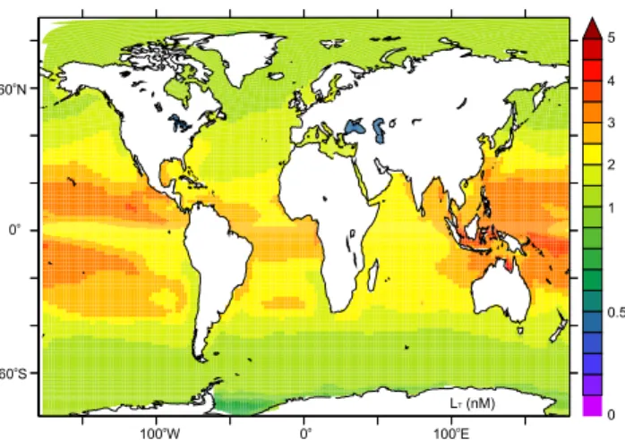
Most OGCBMs assume that the concentration of dFe bind-ing ligands is fixed at between 0.6 and 1 nM and only as-sume one fully bioavailable ligand is present (e.g., Aumont and Bopp, 2006; Moore and Braucher, 2009; Tagliabue et al., 2009; Galbraith et al., 2010). Nevertheless, there is ample experimental evidence of at least two ligand classes and highly variable concentrations (e.g., Buck and Bruland, 2007 Hunter and Boyd, 2007). While parameterizing the sources and sinks of two ligand classes in an OGCBM is perhaps out of reach at this moment (it has been done for a one-dimensional model, Ye et al., 2009), there is some data showing an relationship between ligands and dissolved or-ganic carbon (DOC) concentrations (Wagener et al., 2008, see also: Hiemstra and van Riemsdijk, 2006). We there-fore decided to use the relationship from the observations of Wagener et al. (2008) to permit us to have ligand concen-trations that vary as a function of total DOC concenconcen-trations (DOCTOT, in µmol L−1)that are already prognostically sim-ulated by PISCES).
0 0.5 1 2 3 4 5
60oN
0o
60oS
LT (nM)
100oW 0o 100oE
Fig. 1. The distribution of Fe binding ligands in the upper 100 m when they are computed from an empirical relationship between LTand DOC (Wagener et al., 2008).
3.4 Model experiments
We decided to use our Fe speciation OGCBM to conduct some illustrative model experiments. We firstly simulated Fe chemistry for the “present” climate using an atmospheric CO2 level of 368.87 ppm (corresponding to observations from the year 2000), an ocean circulation from NEMO that arises from atmospheric re-analysis products (Aumont et al., 2008) and depart from a simulation conducted from 1860– 2000 forced by atmospheric CO2observations (to ensure a correct ocean pH). Initially, we used the parameterisation of the Fe cycle as described as above, but we also conducted some illustrative sensitivity tests to examine assumptions re-garding the nature of the variability associated with the Fe binding ligand pool. Finally, in order to appraise the possible impact of climate change on Fe speciation, we used 2 repre-sentations of ocean circulation, as well as initialization files for ocean biogeochemistry (to include the requisite DIC and pH changes), from the IPSL-CM5 coupled model at atmo-spheric CO2 levels of 298.06 ppm and 1086.64 pmm (from a transient coupled simulation from pre-industrial CO2 lev-els to 4×CO2)and conducted 10 year simulations with the Fe speciation analytical solution included in PISCES. Our model experiments are summarized in Table 1. In calcu-lating the bFe concentrations in the following, we test two different assumptions, the first assumes that phytoplankton are not relient on free inorganic species, and thus “bFe” also includes organically complexed Fe. The other assump-tion assumes the contrary, that only free inorganic Fe(II)′ and Fe(III)′ are present as “bioavailable” species and this bFe = Fe(II)′+ Fe(III)′. In a sense, this approach allows us to appraise the degree of Fe limitation experienced by only re-lying on free inorganic Fe species and not making the cellular investment to assimilate organically complexed Fe directly.
4 Results of the model
4.1 Fe speciation from the standard model and comparison with observations
General Fe speciation
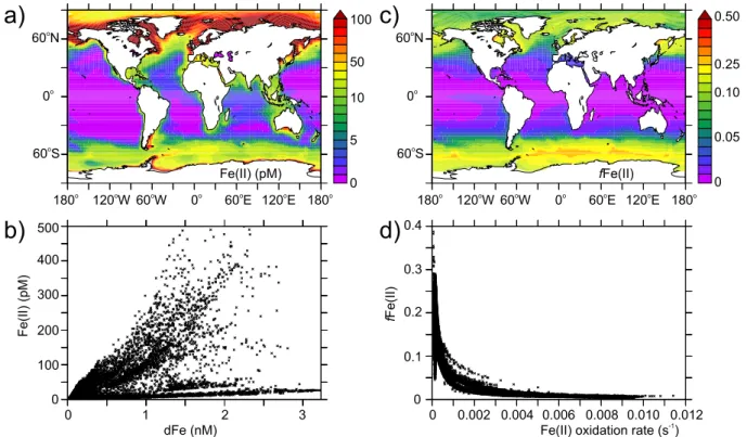
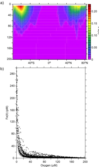
Fig. 2 illustrates the Fe speciation that results from the stan-dard parameterization of our Fe model under modern cli-matic forcing. Annually averaged Fe(II) distributions gen-erally track those of dFe (Fig. 2a and b) and over most of the ocean range between 0 and 100 pM. The annual mean (seasonal variability in fFe(II) is discussed below) propor-tion of the dFe pool present as Fe(II) (fFe(II)) ranges from 0 to around 30 % and is maximal at high latitudes (10–30 %), moderate in upwelling regions (3–4 %) and very low in the tropical oceans (<1 %) (Fig. 2c. For example, fFe(II) in-creases as one moves south in the Southern Ocean from <5 % near South Africa to∼30 % at around 55◦S, with sim-ilar degree of change in the high latitude northern Oceans (Fig. 2c). In general, the latitude-longitude variability in fFe(II) is tightly linked to the variability inkoxfor the surface ocean (Fig. 2d). Irradiance governs the depth distribution of fFe(II), with Fe(II) only making up an appreciable fraction of dFe at depths shallower than∼100 m (Fig. 3a). An exception to this are suboxic zones, wherein the reduction inkox re-sults in Fe(II) levels>100 pM (Fig. 3b, 200–300 m). Organ-ically complexed Fe(III) (FeLSand FeLW)makes up almost 100 % of the dFe pool over most of the global ocean, declin-ing slightly to around 85 % in polar waters where Fe(II) is greater due to supply from photoreduction and reduced oxi-dation rates.
Biovailable Fe
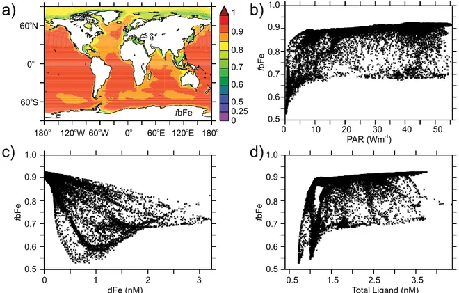
bFe shows variability that is linked to photochemistry, or-ganic complexation and irradiance, as well as being highly sensitive to which species are assumed to be bioavailable. If bFe is assumed to encompass Fe(II), Fe(III) and Fe(III)LS then the proportion of the dFe pool present as bFe (fbFe) varies between 50 to 90 % in surface waters (when annually averaged, Fig. 4a). Variability in fbFe at the surface is posi-tively related to irradiance (due to greater photoproduction of Fe′) and the total ligand concentration (due to reduced losses
Table 1.A summary of the different Fe speciation simulations conducted. Note that for all simulations, the biogeochemical component of the ocean model has been run from the pre-industrial period prior to our Fe speciation tests in order to have an accurate three-dimensional distribution of anthropogenic carbon and thus ocean pH, as well as all other biogeochemical tracers such as the three dimensional distribution of dFe. For CONTROL and FIXED-LIGS, this involved a simulation from 1860 to 2000.
Experiment Ligands Circulation CO2atm (ppm) Duration
CONTROL DOC-linked Climatology 368.87 10 years
FIXED-LIGS Fixed* Climatology 368.87 10 years
PAST DOC-linked IPSL-CM5** 298.06 10 years
FUTURE DOC-linked IPSL-CM5** 1086.64 10 years
∗Ligand concentrations are fixed at 0.6 nM
∗∗Physical fields come from the IPSL coupled climate model, otherwise from the climatological circulation (see text).
60oN
0o
60oS
180o 120oW 60oW 0o 60oE 120oE 180o
60oN
0o
60oS
180o 120oW 60oW 0o 60oE 120oE 180o
0
0 1
dFe (nM) Fe(II) oxidation rate (s-1
)
2 3
100 200 300 400 500
Fe(II) (pM)
f
Fe(II)
0 0.1 0.2 0.3 0.4
0 0.002 0.004 0.006 0.008 0.010 0.012
0 5 10 50 100
0 0.05 0.10 0.25 0.50
a)
b)
c)
d)
Fe(II) (pM) fFe(II)
Fig. 2. Annually averaged surface(a)dissolved Fe(II) (pM) and(b)its relationship to dFe (nM), and(c)the annually average surface proportion of the dFe pool present as Fe(II) (fFe(II)) and(d)its relationship to the oxidation rate constant (s−1).
time for Fe′ (the sum of Fe(II) and Fe(III)) away from po-lar waters and would imply that phytoplankton reliant on Fe′ would be chronically Fe limited in these waters (Tagliabue et al., 2009). Accordingly, fbFe is strongly and negatively related to spatial variability in Fe(II) oxidation rates when bFe = Fe(II)+Fe(III), and thus generally tracks variability in fFe(II).
Importance of seasonality
Seasonality plays an important role in Fe speciation, espe-cially at high latitudes where there are large changes in en-vironmental variables (temperature, irradiance etc, Tagliabue and Arrigo, 2006). During the winter-spring transition in the
0
40
80
120
160
200
40oS 0o 40oN 80oN 0
0.05 0.10 0.15 0.20
fFe(II)
0 40 80 120 160 200 240 280
Fe(II) (pM)
0 40 80 120 160 200 Oxygen (μM)
b) a)
Fig. 3. (a)The zonally averaged fFe(II) for the upper 250 m and
(b)the relationship between Fe(II) and oxygen concentration be-tween 200 and 300 m, highlighting the relative accumulation of Fe(II) in suboxic zones.
Comparison with observations
The most obvious and widespread dataset with which to compare the model is the simulated dFe concentration (from the sum of the Fe species computed by our speciation model). This compares well to a new database of∼13 000 dFe mea-surements (Tagliabue et al., 2011,R=0.52 and 0.54 for the entire water column and 0–50 m, respectively), but although this shows our speciation model does not give unrealistic dFe concentrations in general, the good statistical reproduc-tion of dFe (that arises from our speciareproduc-tion model) probably more reflects the successful simulation of dFe in PISCES. Fe speciation measurements are obviously rarer than those for dFe, but one candidate to compare our speciation model to is Fe(II). At high latitudes, the model appears to do a rea-sonable job, with surface Fe(II) concentrations of∼25 pM
south of New Zealand comparing well with a range of 19– 46 pM from Croot et al. (2007) and modeled values of∼30– 60 pM from the western sub-Arctic Pacific within the range of∼20–40 pM from Roy et al. (2008), with Fe(II) observa-tions making up as much as 50 % of the dFe pool (modeled values are 30–40 %). In addition, the depth profile from Roy et al. (2008) is also relatively well reproduced by the model, except for the reduced attenuation of Fe(II) with depth in the model (Fig. 7). Earlier Southern Ocean observations of 0–45 pM using a towed fish (Bowie et al., 2002) are also reasonably well reproduced by the model. A widespread Fe(II) dataset was obtained by Sarthou et al. (2011) along the Bonus-GoodHope transect in the Southern Ocean and using the parallel dFe measurements (Chever et al., 2010) permits us to derive fFe(II). Our model has a similar trend in the gen-eral values of surface Fe(II) observed in the Southern Ocean (0–40 pM vs. 12–116 pM), as well as the increasing south-ward trend along the Bonus-GoodHope line (Sarthou et al., 2011). In addition, fFe(II) from the model (0–30 % increas-ing southward) agrees well with the observations (3–67 %, Sarthou et al., submitted). It is noteworthy, that the observed latitudinal trends in both Fe(II) and fFe(II) were only sig-nificant for daytime stations (Fe(II)) and for both daytime and all stations (fFe(II)), but never when only night-time sta-tions were considered (Sarthou et al., 2011). In the east-ern North Atlantic, the onshore-offshore trend (from>250 to 100–150 pM) observed by Boye et al. (2003) is similar to that in the model and observed offshore values (∼100 pM) are, in general, only slightly underestimated by the model (although the limit of detection in Boye et al. (2003) was 100 pM). This is probably due to the onshore-offshore trend in dFe concentrations, since we do not include a specific source of Fe(II) at the margin (there is a margin source of dFe in PISCES). High modeled Fe(II) levels in the Baltic Sea agree well with measurements of Breitbarth et al. (2009). In general, this suggests that the model is reasonably well repro-ducing the dominant processes governing the Fe(II) distribu-tion in higher latitude Atlantic, Pacific and Southern Oceans. It is worth noting that Fe(II) as a transient species shows sig-nificant variability on short time and space scales (e.g., Croot et al., 2007; Roy et al., 2009) and it is for this reason that we evaluated the general trends in the modelled Fe(II) concen-trations rather than comparing the model and observations “point by point” (where a model error in mixed layer depth, temperature, light etc could drive a deviation from observa-tions that is not due to the speciation model per se).
60o
N
0o
60o
S
180o
120o
W 60o
W 0o
60o
E 120o
E 180o
0 0.25 0.5 0.6 0.7 0.8 0.9 1
0 10 20 30 40 50
PAR (Wm-1
) 0.5
0.6 0.7 0.8 0.9 1.0
f
bFe
0.5 0.6 0.7 0.8 0.9 1.0
f
bFe
0.5 0.6 0.7 0.8 0.9 1.0
f
bFe
0 1
dFe (nM)
2 3 0.5 1.5 2.5 3.5
Total Ligand (nM)
a)
c)
b)
d)
fbFe
Fig. 4. The(a)annual maximum surface proportion of the dFe pool present as bFe and its relationship to(b)irradiance (Wm−2),(c)the total concentration of ligands (nM) and d) the dFe concentration (nM), when bFe is assumed to equal Fe(II) + Fe(III) + FeLS.
60o
N
0o
60o
S
180o
120o
W 60o
W 0o
60o
E 120o
E 180o
0 0.1 0.2 0.3 0.4 0.5
fbFe
Fig. 5. The annually averaged proportion of the dFe pool present as bFe pool when bFe is assumed to only equal Fe(II) + Fe(III) (compare to Fig. 4a).
a lack of high frequency output, or the absence of the diur-nal cycle in PISCES. The method employed by Hansard et al. (2009) is based on acidified samples and therefore likely reflects a labile Fe′ pool that is highly sensitive to redox conditions. Unfortunately, the dFe measurements taken par-allel to the Hansard et al. (2009) Fe(II) measurements are not yet available and it is not possible to directly compare fFe(II) from the model and observations (which would tell
40o
N 80o
N
40o
S 0o
40oN
80o
N
40o
S 0o
0 0.05 0.10 0.20 0.30 0.40
0.5 0.56 0.62 0.68 0.74 0.8 0.88 0.92 0.98
f
Fe(II)
f
bFe
a)
b)
JAN FEB MAR APR MAY JUN JUL AUG SEP OCT NOV DEC
Fig. 6.Seasonal variability (monthly averages) in the zonally aver-aged proportion of the dFe pool present as(a)Fe(II) and(b)bFe.
0 0
20
30
40
10 20 30 40 50
Model Profile 8-4 Profile 8-14 Fe(II) (pM)
Depth (m)
Fig. 7. A profile of modeled Fe(II) alongside profiles 8–4 (47◦ 35.852′N 165◦58.760′E) and 8–14 (47◦51.220′N 166◦15.244′E) presented in Roy et al. (2008).
and 100 pM and are therefore very low, relative to the Fe(II) concentrations measured by Hansard et al. (2009), which are of the same order. This suggests it would be very difficult to achieve any appreciable Fe(II) in this region whilst mod-eled dFe values remain so low. Additional sensitivity tests focused on producing more Fe(II) in this region (drastically reducingkoxor increasing photoreduction, not shown) do not permit any appreciable accumulation of Fe(II) therein and re-sult in unrealistically high Fe(II) concentrations in the high latitudes. Fe(II) might also be underestimated in the lower latitude ocean because the diurnal cycle in irradiance is not included in our OGCBM. Another important issue to bear in mind is that we compare point measurements to the monthly mean model output. Models and observations (e.g., Bowie et al., 2002; Tagliabue and Arrigo, 2006; Croot et al., 2007, 2008; Roy et al., 2008; Breitbarth et al., 2009; Ye et al., 2009; Sarthou et al., 2011) show a high degree of variability in Fe(II) in response to changing environmental conditions (especially solar radiation on the diel cycle), although it is noticeable that Hansard et al. (2009) note no diurnal cycle in their observations, in contrast to other studies. Our model may not capture these “extreme” events that are highly spe-cific to the time and location of each precise sample. This is because despite a 1.5 h timestep, we do not include the diur-nal cycle and compare monthly mean modeled Fe(II) to point measurements. Therefore, we must conclude that a combina-tion of a very low modeled dFe concentracombina-tion, lack of high frequency variability and perhaps also an impact of acidified samples and errors in our formulated Fe cycle (see below) precludes a good reproduction of the reported Fe(II) data in the subtropical Pacific Ocean (Fe(II) levels are higher in the tropical Atlantic due to greater dust input of dFe). However we do note the increased Fe(II) in suboxic zones (Fig. 3b), in the eastern tropical Pacific in particular, that compare well to measured increases in Fe(II) at low oxygen levels (e.g., Hopkinson and Barbeau, 2007).
As regards the degree of organic complexation, our re-sults of virtually 100 % complexation of dFe agrees with
60o
N
0o
60o
S
180o
120o
W 60o
W 0o
60o
E 120o
E 180o
60o
N
0o
60o
S
180o
120o
W 60o
W 0o
60o
E 120o
E 180o
180o
120o
W 60o
W 0o
60o
E 120o
E 180o
a)
b)
c)
0 0.2 0.4 0.6
-0.6 -0.4 -0.2 -0.1 0
-0.7 -0.5 -0.3
-0.1 0
-0.7 -0.5 -0.3
Fig. 8. The proportional change (i.e., (Xfixlig – Xvarlig)/Xvarlig) in the proportion of the dFe pool (a) organically complexed,
(b) present as bFe when bFe = Fe(II) + Fe(III) + FeLS and
(c)present as bFe when bFe = Fe(II) + Fe(III) when ligands are assumed to be fixed at 0.6 nM.
all available observations (e.g., Boye et al., 2003; Boye et al., 2006; Buck and Bruland, 2007) and lesser complexation where Fe inputs are high is in accord with the findings from an artificial Fe enrichment experiment (Boye et al., 2005). Overall, our speciation model can be seen to do a much bet-ter job at higher latitudes, rather than lower latitudes without significant Fe inputs (where Fe(II) levels appear too low).
Sensitivity tests
concentration unsurprisingly results in a reduction in the pro-portion of the total dFe pool that is organically complexed (Fig. 8a). This then impacts the total dFe pool, which is re-duced (due to greater losses as FeP), especially in regions of high Fe inputs (beneath zones of dust deposition and near coasts). The impact of fixed (and generally lower) ligand concentrations upon bFe depends on the assumed make up of the bFe pool. If bFe = Fe(II)+Fe(III)+FeLS, then bFe de-clines if ligands are fixed (Fig. 8b), due to reduced stabiliza-tion of bFe by LS (as its concentration is reduced). On the other hand, if bFe is assumed to be only made up of Fe(II) and Fe(III), then assuming lower and fixed ligand concen-trations actually increases bFe (albeit from very low levels, Fig. 8c), particularly in areas of high Fe input, due to lesser complexation by organic ligands (which are assumed inac-cessible to phytoplankton in this formulation of bFe). Thus the nature of the ocean ligand pool has impacts upon the general speciation of Fe, as well as its residence time and bioavailability. We reiterate that for phytoplankton that can access organically complexed Fe, bFe declines when ligands are fixed (at generally lower levels than measured), while for phytoplankton reliant on inorganic Fe, bFe increases when ligands are fixed since more Fe is in inorganic forms.
4.2 Fe speciation at four times CO2
At atmospheric CO2levels of approximately 1000 ppm the environmental properties of the ocean are unsurprisingly greatly modified. In general, and similar to previous stud-ies with fully coupled climate-OGCBMs (e.g., Steinacher et al., 2010), the surface ocean is warmer, more stratified (re-duced mixed layer depth) and has a lower pH. In the South-ern Ocean, sea ice coverage is also reduced which lengthens the growing season. Our objective here is not to comprehen-sively analyze these aspects (this is for other more focused papers), but to examine how Fe speciation changes using our analytical approach.
Turning firstly to Fe(II), we find large increases in fFe(II) (chosen to remove the effect of climate on absolute dFe con-centrations) due to climate change that are maximal in the high latitude oceans (Figure). fFe(II) increases by as much as>40 % in the high latitude Southern and Northern Oceans (Fig. 9a) and must be responding to changes to oxidation and photoreduction rates. However, a closer inspection reveals that the largest changes in fFe(II) occur where photoreduc-tion rates were not significantly changed and that there is a very close relationship between the predicted changes to fFe(II) and oxidation rates (Fig. 9b). This suggests that the impact of reduced pH is overriding the impact of greater tem-perature to yield a net reduction in the future oxidation rate of Fe(II), especially in the high latitude oceans. Similar accu-mulations of Fe(II) at lower pH were obtained in mesocosm experiments by Breitbarth et al. (2010), where pH changes impacting oxidation rates were also found to be the domi-nant effect.
60o
N
0o
60o
S
180o
120o
W 60o
W 0o
60o
E 120o
E 180o
60o
N
0o
60o
S
180o
120o
W 60o
W 0o
60o
E 120o
E 180o
60o
N
0o
60o
S
180o
120o
W 60o
W 0o
60o
E 120o
E 180o
0
-0.1
-0.2 0.2
0.1
0
-0.2
-0.4 0.4
0.2 0,2
0.1
0 0.4
0.3
0,2
0.1
0 0.4
0.3
Proportional
Δ
Fe(II)
-0.8 -0.4 0 0.4
Proportional ΔKox
a)
c)
b)
d)
ΔfFe(II)
ΔfbFe ΔfbFe
Fig. 9. The proportional (i.e., (Xhigh CO2 – Xlow CO2)/Xlow CO2)change in the (a)proportion of the dFe pool present as Fe(II) at an atmospheric CO2level of∼1000 ppm and(b)its relationship to the proportional change in the oxidation rate constant, and the proportional change in the proportion of the dFe pool present as bFe pool when bFe equals(c)Fe(II) + Fe(III) + FeLSand(d)Fe(II) + Fe(III).
5 Future directions
5.1 Improvements to the speciation model
While our Fe speciation model is complex, relative to con-temporary treatments of Fe cycling in global OGCBMs, there are a number of simplifications and processes that could be included/tested in the future. For example, processes such as Fe(III) reduction as mediated by superoxide, the direct photoreduction of Fe(III) and Fe(III) colloids, as well as including the role of superoxide and hydrogen peroxide in the oxidation of Fe(II) could also be important in govern-ing the spatio-temporal variability in Fe(II) concentrations. The Fe speciation model of Ye et al. (2009) is a good candi-date model with which to explore the potential importance of such processes. However, as this model is even more complex than our Fe speciation model, it cannot be solved analytically anymore. Nevertheless, an iterative numerical solution is possible and leads to vast savings in computa-tional time compared to solving the full kinetic equations in the one-dimensional setting by Ye et al. (2009) (V¨olker et al., 2011). A good candidate addition to the current spe-ciation model that would not overcomplicate the analytical solution might be Fe(II) ligands, which could assist in re-producing the relatively high Fe(II) suggested in the low lat-itudes (e.g., Hansard et al., 2009). The presence of Fe(II)
ligands, including perhaps those specific to Fe(II), cycling of colloidal Fe and questions regarding Fe bioavailability (see below).
5.2 Modeling Fe binding ligands
We have shown that variability in ocean Fe binding lig-ands exert a critical control on the speciation of dFe and, as such, on the residence time and bioavailability of dFe. Here we have used the semi-labile DOC pool as simulated by PISCES, alongside a relationship derived from field ob-servations (Wagener et al., 2008) to allow ligands to vary in our model. However, while this is likely to be a cost effec-tive improvement upon a fixed uniform ligand concentration (as currently employed in other OGCBMs), it will be impor-tant to carefully compare the distribution with widespread in situ ligand data to better constrain its viability. For example, while our DOC-linked parameterization will account for lig-and production in surface waters, remineralisation (Boyd et al., 2010; Ibisanmi et al., 2011) is not a source of ligands and it absence in our parameterization may hinder the reproduc-tion of subsurface peaks in ligand concentrareproduc-tions (Boye et al., 2010; Ibisanmi et al., 2011; Thuroczy et al., 2011). In the fu-ture it may be useful to include a prognostic simulation of the production of weak ligands from organic matter breakdown, as well as the production of strong ligands by the biota, pos-sibly mediated by Fe stress as per Ye et al. (2009), which could be then compared against ligand profiles. A prognos-tic ligand model would need to be simulated as part of the “slow” Fe cycle reactions and thus require a long model spin up (order of hundreds to thousands of years) in order to cor-rectly simulate deep water concentrations. But this would be feasible in a 3-D global OGCBM, since it would only re-quire the addition of two new tracers (LW and LS). To that end, more data on the concentrations (especially their pro-files, e.g., Boye et al., 2010; Thuroczy et al., 2011; Ibisanmi et al., 2011) and binding strengths of ocean binding ligands will prove invaluable.
5.3 Impact of climate and pH on Fe speciation
While our Fe speciation model has difficulties in reproducing the Fe(II) concentrations measured by Hansard et al. (2009, notwithstanding metholodogical issues), our model does a good job in the regions we predict to be impacted by climate change and ocean acidification (the high latitudes). It will be necessary to carefully understand the reasons behind the low modeled dFe concentrations in the tropical Pacific as this cer-tainly restricts the accumulation of Fe(II) therein. Our model suggests that ocean acidification, rather than climate, is likely to exert the strongest control on the evolution of Fe speciation (independent of any effects on absolute dFe concentrations) over the coming century through its mediation of redox ki-netics. The greater fraction of Fe(II) we simulate agrees with results from mesocosm experiments using natural seawater
with bubbled CO2(Breitbarth et al., 2010). Laboratory re-sults using synthetic ligands have shown that the complexa-tion of Fe′by ligands could also change with ocean
acidifi-cation as a function of the degree of protonation of a given ligand, with increases, decreases and no change in complexa-tion possible (Shi et al., 2010). If the in situ ocean ligand pool can be better characterized, and perhaps connected to dif-ferent production pathways (sensu Hunter and Boyd, 2007), then we could test the combined impact of climate and pH on Fe redox speciation and ligand complexation/cycling in the future. For example, if remineralization is an important source of Fe binding ligands (Boyd et al., 2010; Ibisanmi et al., 2011), then it may be important to understand climate impacts on ligand production rates, as well as their vertical supply from the subsurface to the surface ocean, in concert with effects on Fe redox speciation and potential “direct” ef-fects of pH on organic complexation.. Nevertheless, we note that understanding the ultimate impact on the biota will crit-ically depend on the assumptions regarding the nature of the in situ bFe pool. Reducing the uncertainties associated with the costs and benefits of phytoplankton assimilating different Fe species is crucial.
5.4 Modeling Fe bioavailability
result (if any). In doing so, we will be better able to eval-uate the impact of climate driven changes in Fe speciation (on multiple timescales) on phytoplankton productivity and growth rates.
6 Conclusions
Using an analogy with the computation of inorganic carbon speciation in OGCBMs, we outline a means by which Fe spe-ciation can be solved analytically in a cost effective manner in global models. Our approach rests on the division of the Fe cycle into “fast” and “slow” reactions and permits us to simulate 3D Fe speciation using a global OGCBM. We use our model to show that the distribution of different Fe species is tightly controlled by the dFe concentration, the distribution and concentrations of Fe-binding ligands and environmental variables (temperature, light, oxygen and pH). When com-pared directly to measurements of Fe(II), our model does a reasonable job of reproducing observations in the high lat-itude oceans (notwithstanding the variability of measured Fe(II) on short time and space scales), but appears to sys-tematically underestimates Fe(II) in the low latitude Pacific Ocean (although these may be overestimated). This could result from errors in the modeled dFe field, the absence of the diurnal cycle and high frequency variability, or missing processes from our Fe cycle model (such as Fe(II) binding ligands or specific Fe(II) sources). Using our model under future climate suggests that climate change and, in particu-lar, ocean acidification will impact Fe cycling and speciation, especially in the Fe limited Southern Ocean. We predict sig-nificant increases in Fe(II) due to acidification, which could reduce the “Fe limited area” of the Southern Ocean by∼20 % for species that rely solely on assimilating on inorganic Fe. We speculate that a dFe pool that has an increased ‘free’ inor-ganic component might exert a selective pressure on compet-itive Fe uptake strategies exhibited by phytoplankton in the future ocean. Finally, our ’analytical solution’ approach can be used as a framework within which to test our understand-ing of Fe speciation at the global scale in future studies if desired. As such, it can provide a means by which new mea-surements of Fe speciation can be evaluated against hypothe-ses regarding the quantitative formulation of the proceshypothe-ses at play in the ocean’s Fe cycle.
Acknowledgements. The collaboration necessary to initialize this work was formed during two EU COST action (735) workshops in Kiel, Germany, organized by P. Croot. We thank P. Croot and all the participants of these workshops for their input and support. In addition, we specifically thank M. Santana-Casiano and M. Gonz´alez D´avila for providing their oxidation rate equation and help with its implementation, T. Wagener for providing the DOC – ligand equation, K. Barbeau, M. Boye, P. Croot, S. Hansard, and M. Wells for kindly providing published Fe(II) datasets, while G. Sarthou generously provided unpublished Bonus-GoodHope Fe(II) observations and insightful comments on the manuscript,
and A. Caubel for assistance with the implementation of the analytical Fe chemistry in NEMO-PISCES. Additional ideas and discussions with K. Arrigo, O. Aumont, A. Bowie, L. Bopp, M. Gehlen, M. Lohan, G. Sarthou, P. Sedwick and Y. Ye were greatly appreciated. A. T. and C. V. acknowledge funding by the “Euro-pean Project of Ocean Acidification (EPOCA, grant agreement no. 211384) and “Africa Centre for Climate and Earth Systems Science” (ACCESS) and “Surface processes in the anthropocene” (SOPRAN, grant agreement 03F0462C), respectively. This work was carried out using HPC resources from GENCI-IDRIS (Grant 2009-10040). We thank two anonymous reviewers and the editor for their comments, which have improved the manuscript.
Edited by: C. P. Slomp
The publication of this article is financed by CNRS-INSU.
References
Aumont, O. and Bopp, L.: Globalizing results from ocean in situ iron fertilization studies, Global Biogeochem. Cy., 20, GB2017, doi:10.1029/2005GB002591, 2006.
Aumont, O., Orr, J., Monfray, P., Ludwig, W., Amiotte-Suchet, P., and Probust, J. L.: Riverine-Driven Interhemispheric Transport of Carbon, Global Biogeochem. Cy., 15, 393–405, 2001. Aumont, O., Bopp, L., and Schulz, M.: What does temporal
vari-ability in aeolian dust deposition contribute to sea-surface iron and chlorophyll distributions?, Geophys. Res. Lett., 35, L07607, doi:10.1029/2007GL031131, 2008.
Barbeau, K., E. L. Rue, C. G. Trick, K. W. Bruland, and A. But-ler: Photochemical reactivity of siderophores produced by ma-rine hetero-trophic bacteria and cyanobacteria based on charac-teristic Fe(III) binding groups, Limnol. Oceanogr., 48, 1069 – 1078, 2003.
Boyd, P. W., Jickells, T., Law, C. S., Blain, S., Boyle, E. A., Buesseler, K. O., Coale, K. H., Cullen, J. J., de Baar, H. J., Follows, M., Harvey, M., Lancelot, C., Levasseur, M., Owens, N. P., Pollard, R., Rivkin, R. B., Sarmiento, J., Schoemann, V., Smetacek, V., Takeda, S., Tsuda, A., Turner, S., and Wat-son, A. J.: Mesoscale iron enrichment experiments 1993–2005: synthesis and future directions, Science, 315, 5812, 612–617, doi:10.1126/science.1131669, 2007.
Boyd, P. W., Ibisanmi, E., Sander, S. G., Hunter, K. A., and Jack-son, G. A.: Remineralization of upper ocean particles: Impli-cations for iron biogeochemistry, Limnol. Oceanogr., 55, 1271– 1288, 2010.
Boye, M., Nishioka, J., Croot, P. L., Laan, P., Timmermans, K. R., and de Baar, H. J. W.: Major deviations of iron complexation dur-ing 22 days of a mesoscale iron enrichment in the open Southern Ocean, Mar. Chem., 96, 257–271, 2005.
Boye, M., Aldrich, A., van den Berg, C. M. G., De Jong, J. T. M., Nirmaier, H., Veldhuis, M., Timmermans, K. R., and de Baar, H. J. W.: The chemical speciation of iron in the north-east Atlantic Ocean, Deep Sea Res. Pt. I, 53, 667–683, doi:10.1016/j.dsr.2005.12.015, 2006.
Boye, M., Nishioka, J., Croot, P., Laan, P., Timmermans, K. R., Strass, V. H., Takeda, S., and de Baar, H. J. W.: Significant por-tion of dissolved organic Fe complexes in fact is Fe colloids, Mar. Chem., doi:10.1016/j.marchem.2010.09.001, 2010.
Breitbarth, E., Gelting, J., Walve, J., Hoffmann, L. J., Turner, D. R., Hassell´ov, M., and Ingri, J.: Dissolved iron (II) in the Baltic Sea surface water and implications for cyanobacterial bloom devel-opment, Biogeosciences, 6, 2397–2420, doi:10.5194/bg-6-2397-2009, 2009.
Breitbarth, E., Bellerby, R. J., Neill, C. C., Ardelan, M. V., Meyerh¨ofer, M., Z¨ollner, E., Croot, P. L., and Riebesell, U.: Ocean acidification affects iron speciation during a coastal sea-water mesocosm experiment, Biogeosciences, 7, 1065–1073, doi:10.5194/bg-7-1065-2010, 2010.
Boukhalfa, H. and Crumbliss, A. L.: Chemical aspects of siderophore mediated iron transport, Biometals, 15, 325–339, 2002.
Buck, K. N. and K. W.: Bruland: The physiochemical speciation of dissolved iron in the Bering Sea, Alaska, Limnol. Oceanogr., 52, 1800–1808, 2007.
Buitenhuis, E. T. and Geider, R. J.: A model of phytoplankton ac-climation to iron-light colimitation, Limnol. Oceanogr., 55, 714– 724, 2010.
Croot, P., Bowie, A., Frew, R., Maldonado, M., Hall, J., Safi, K., LaRoche, J., Boyd, P., and Law, C.: Retention of dissolved iron and FeII in an iron induced Southern Ocean phytoplankton bloom, Geophys. Res. Lett., 28, 3425–3428, 2001.
Croot, P. L., Frew, R. D., Sander, S., Hunter, K. A., Ell-wood, M. J., Abraham, E. R., Law, C. S., Smith, M. J., and Boyd, P. W.: The effects of physical forcing on iron chemistry and speciation during the FeCycle experiment in the South West Pacific, J. Geophys. Res.-Oceans, 112, C06015, doi:06010.01029/02006JC003748, 2007.
Croot, P. L., Bluhm, K., Schlosser, C., Streu, P., Breitbarth, E., Frew, R., and Van Ardelan, M.: Regeneration of Fe(II) during EIFeX and SOFeX, Geophys. Res. Lett., 35, L19606, doi:10.1029/2008GL035063, 2008.
Cullen, J. T., Bergquist, B. A., and Moffat, J. W.: Thermodynamic characterization of the partitioning of iron between soluble and colloidal species in the Atlantic Ocean, Mar. Chem., 98, 295– 303, doi:10.1016/j.marchem.2005.10.007, 2006.
Flynn, K. J.: Modelling multi-nutrient interactions in phytoplank-ton; balancing simplicity and realism, Prog. Oceanogr., 56, 249– 279, 2003.
Galbraith, E. D., Gnanadesikan, A., Dunne, J. P., and His-cock, M. R.: Regional impacts of iron-light colimitation in a global biogeochemical model, Biogeosciences, 7, 1043–1064, doi:10.5194/bg-7-1043-2010, 2010.
Gledhill, M. and van den Berg, C. M. G.: Determination of the complexation of Fe(III) with natural organic complexing ligands
in seawater using cathodic stripping voltammetry, Mar. Chem., 47, 41–54, doi:10.1016/0304-4203(94)90012-4, 1994.
Hansard, S. P., Landing, W. M., Measures, C. I., and Voelker, B. M.: Dissolved iron(II) in the Pacific Ocean: Measurements from the PO2and P16N CLIVAR/CO2repeat hydrography expeditions, Deep Sea Res. Pt. I, 56, 1117–1129, 2009
Hiemstra, T. and van Riemsdijk, W. H.: Biogeochemical spe-ciation of Fe in ocean water, Mar. Chem., 102, 181–197, doi:10.1016/j.marchem.2006.03.008, 2006.
Hudson, R. and Morel, F. M. M.: Iron transport in marine phy-toplankton: Kinetics of cellular and medium coordination reac-tions, Limnol. Oceanogr., 35, 1002–1020, 1990.
Hunter, K. A. and Boyd, P. W.: Iron-binding ligands and their role in the ocean biogeochemistry of iron, Environ. Chem., 4, 221–232, 2007.
Hutchins, D. A., Witter, A. E., Butler, A., and Luther III, G. W.: Competition among marine phytoplankton for different chelated iron species, Nature, 400, 858–861, doi:10.1038/23680, 1999. Ibisanmi, E., Sander, S. G., Boyd, P. W., Bowie, A. R., and
Hunter, K. A.: Vertical Distributions of Iron-(III) Complex-ing Ligands in the Southern Ocean, Deep Sea Res. Pt. II, doi:10.1016/j.dsr2.2011.05.028, in press, 2011.
Maldonado, M. and Price, N.: Utilization of iron bound to strong organic ligands by plankton communities in the subarctic North Pacific, Deep Sea Res. Pt. II, 46, 2447–2473, 1999.
Maldonado, M. T. and Price, N. M.: Reduction and transport of organically bound iron by Thalassiosira oceanica (Bacillario-phyceae), J. Phycol., 37, 298–309, 2001.
Maldonado, M. T., Allen, A. E., Chong, J. C., Lin, K., Leus, D., Karpenko, N., and Harris, S.: Copper dependent iron transport in coastal and oceanic diatoms, Limnol. Oceanogr., 51, 1729–1743, 2006.
Moog, P. and Br¨uggemann, W.: Iron reductase systems on the plant plasma membrane – A review, Plant Soil, 165, 241–260, 1994. Moore, J. K. and Braucher, O.: Sedimentary and mineral dust
sources of dissolved iron to the world ocean, Biogeosciences, 5, 631–656, doi:10.5194/bg-5-631-2008, 2008.
Morel, F. M. M., Kustka, A. B., and Shaked, Y.: The role of unchelated Fe in the iron nutrition of phytoplankton, Limnol., Oceanogr., 53, 400–404, 2008.
Parekh, P., Follows, M., and Boyle, E.: Modelling the global ocean iron cycle, Global Biogeochem. Cy., 18, GB1002, doi:10.1029/2003GB002061, 2004.
Raven, J. A.: The iron and molybdenum use efficiencies of plant growth with different energy, carbon and nitro-gen sources, New Phytol., 109, 279–287, doi:10.1111/j.1469-8137.1988.tb04196.x, 1988.
Raven, J. A., Evans, M. C. W., and Korb, R. E.: The role of trace metals in photosynthetic electron transport in O2-evolving organisms, Photosynth. Res., 100, 111–150, doi:10.1023/A:1006282714942, 1999.
Rose, A. and Waite, T.: Effect of dissolved natural organic matter on the kinetics of ferrous iron oxygenation in seawater, Environ. Sci. Technol., 37, 4877–4886, 2003.
model of iron acquisition: Nondissociative reduction of ferric complexes in the marine environment, Limnol. Oceanogr., 51, 1744–1754, 2006.
Santana-Casiano, J. M., Gonzalez-Davila, M., and Millero, F. J.: Oxidation of nanomolar levels of Fe(II) with oxygen in natural waters, Environ. Sci. Technol., 39, 2073–2079, 2005.
Sarmiento, J. L., Slater, R., Barber, R., Bopp, L., Doney, S. C., Hirst, A. C., Kleypas, J., Matear, R., Mikolajewicz, U., Monfray, P., Soldatov, V., Spall, S. A., and Stouffer, R.: Response of ocean ecosystems to climate warming, Global Biogeochem. Cy., 18, GB3003, doi:10.1029/2003GB002134, 2004.
Shaked, Y., Kustka, A. B., and Morel, F. M. M.: A general kinetic model for iron acquisition by eukaryotic phytoplankton, Limnol. Oceanogr., 50, 872–882, 2005.
Shi, D., Xu, Y., Hopkinson, B., and Morel, F. M. M.: Effect of Ocean Acidification on Iron Availability to Marine Phytoplank-ton, Science, 327, 5966, 676–679, doi:10.1126/science.1183517, 2010.
Strzepek, R. F. and Harrison, P. J.: Photosynthetic architecture differs in coastal and oceanic diatoms, Nature, 431, 689–392, doi:10.1038/nature02954, 2004.
Tagliabue, A. and Arrigo, K. R.: Processes governing the supply of iron to phytoplankton in stratified seas, J. Geophys. Res., 111, C06019, doi:10.1029/2005JC003363, 2006.
Tagliabue, A., Bopp, L., Aumont, O., and Arrigo, K. R.: Influence of light and temperature on the marine iron cycle: From theoret-ical to global modeling, Global Biogeochem. Cy., 23, GB2017, doi:10.1029/2008GB003214, 2009.
Takahashi, T., Sutherland, S., Wanninkhof, R., Sweeney, C., Feely, R., Chipman, D., Hales, B., Friederich, G., Chavez, F., Sabine, C., Watson, A., Bakker, D., Schuster, U., Metzl, N., Yoshikawa-Inoue, H., Ishii, M., Midorikawa, T., Nojiri, Y., K¨ortzinger, A., Steinhoff, T., Hoppema, M., Olafsson, J., Arnarson, T., Tilbrook, B., Johannessen, T., Olsen, A., Bellerby, R., Wong, C., Delille, B., Bates, N., and de Baar, H.: Climatological mean and decadal change in surface oceanpCO2, and net sea-air CO2 flux over the global oceans, Deep Sea Res. Pt. II, 56, 554–577, doi:10.1016/j.dsr2.2008.12.009, 2009.
Thuroczy, C., Gerringa, L. J. A., Klunder, M. B., Laan, P., and de Baar, H. J. W.: Observation of consistent trends in the organic complexation of dissolved iron in the At-lantic sector of the Southern Ocean, Deep Sea Res. Pt. II, doi:10.1016/j.dsr2.2011.01.002, 2011.
Van den Berg C.: Evidence for organic complexation of iron in sea-water, Mar. Chem., 50, 139–157, 1995.
Voelker, B. and Sulzberger, B.: Effects of fulvic acid on Fe(II) oxi-dation by hydrogen peroxide, Environ. Sci. Technol., 30, 1106– 1114, 1996.
V¨olker, C. and Wolf-Gladrow, D. A.: Physical limits on iron uptake mediated by siderophores or surface reductases, Mar. Chem., 65, 227–244, 1999.
Wagener, T., Pulido-Villena, E., and Guieu, C.: Dust iron dis-solution in seawater: Results from a one-year time-series in the Mediterranean Sea, Geophys. Res. Lett., 35, L16601, doi:10.1029/2008GL034581, 2008.
Weber, L., V¨olker, C., Schartau, M., and Wolf-Gladrow, D. A.: Modeling the speciation and biogeochemistry of iron at the Bermuda Atlantic Time-series Study site, Global Biogeochem. Cy., 19, GB1019, doi:10.1029/2004GB002340, 2005.
Weber, L., V¨olker, C., Oschlies, A., and Burchard, H.: Iron pro-files and speciation of the upper water column at the Bermuda Atlantic Time-series Study site: a model based sensitivity study, Biogeosciences, 4, 689–706, doi:10.5194/bg-4-689-2007, 2007. Willey, J. D., Kieber, R. J., Seaton, P. J., and Miller, C.: Rainwa-ter as a source of Fe(II)-stabilizing ligands to seawaRainwa-ter, Limnol. Oceanogr., 53, 1678–1684, 2008
Witter, A. E., Hutchins, D. A., Butler, A., and Luther III, G. W.: Determination of conditional stability constants and kinetic con-stants for strong model Fe-binding ligands in seawater, Mar. Chem., 69, 1–17, doi:10.1016/S0304-4203(99)00087-0, 2000. Wu, J., Boyle, E. A., Sunda, W., and Wen, L. S.: Soluble and
colloidal iron in oligotrophic North Atlantic and North Pacific oceans, Science, 293, 847–849, 2001.
Wu, J. and Luther III, G. W.: Complexation of Fe(III) by organic ligands in the northwest Atlantic Ocean by a competitive ligand equilibration method and a kinetic approach, Mar. Chem., 50, 159–177, 1995.