FUNDAÇÃO GETULIO VARGAS
ESCOLA DE ECONOMIA DE SÃO PAULO
GUILHERME DE OLIVEIRA KATER
OPTIMAL MONETARY POLICY UNDER ADMINISTERED
PRICES
GUILHERME DE OLIVEIRA KATER
OPTIMAL MONETARY POLICY UNDER ADMINISTERED
PRICES
Dissertação apresentada à Escola de Economia de São Paulo da Fundação Getulio Vargas (FGV/EESP) como requisito para a obtenção do título de Mestre em Economia.
Campo de Conhecimento: Macroeconomia
Orientador: Prof. Dr. Vladimir Teles
Kater, Guilherme de Oliveira.
Optimal Monetary Policy Under Administered Prices / Guilherme de Oliveira Kater. - 2015.
117 f.
Orientador: Vladimir Kühl Teles
Dissertação (MPFE) - Escola de Economia de São Paulo.
1. Política monetária – Modelos matemáticos. 2. Equilíbrio econômico. 3. Preços. 4. Taxas de juros. I. Teles, Vladimir Kühl. II. Dissertação (MPFE) - Escola de Economia de São Paulo. III. Título.
GUILHERME DE OLIVEIRA KATER
OPTIMAL MONETARY POLICY UNDER ADMINISTERED
PRICES
Dissertação apresentada à Escola de Economia de São Paulo da Fundação Getulio Vargas (FGV/EESP) como requisito para a obtenção do título de Mestre em Economia.
Orientador: Prof. Dr. Vladimir Teles Data de Aprovação:
Banca Examinadora:
Prof. Dr. Vladimir Teles
Dr. Sergio Lago
Prof. Dr. Bernardo Guimarães
AGRADECIMENTOS
O primeiro agradecimento é para minha esposa, Eva, e para minha filha, Alice, que durante este longo período, e por serem as pessoas mais especiais da minha vida, tiveram comigo toda a paciência, compreensão e carinho que eu precisava.
Ao prof. Aidar e prof. Nakano pela bolsa de estudo e apoio para atingir esta meta pessoal e profissional.
Ao meu orientador, Prof. Dr. Vladimir Teles, pelas discussões, por todo o suporte e por acreditar neste trabalho.
Ao Celso pelas importantes dicas e pelo tempo dispendido para me ajudar a entender os modelos DSGE.
Aos meus colegas de trabalho pela colaboração e pela paciência por me aturarem enquanto derivava as intermináveis equações deste trabalho.
Aos meus pais e minha família, pelo apoio e compreensão por estes e todos os momentos até hoje.
RESUMO
Este trabalho tem o objetivo de analisar a interação e os efeitos dos preços administrados na economia, por meio de um modelo DSGE e pela derivação das políticas monetárias ótimas.
O modelo utilizado é um modelo DSGE padrão Novo Keynesiano de uma economia fechada com empresas de dois setores, no primeiro setor, de preços livres, há um contínuo de empresas, e no setor de preços administrados uma única empresa. Adicionalmente, o modelo possui inflação positiva no steady state.
Os resultados do modelo sugerem que os movimentos de preços em qualquer setor terá impacto em ambos os sectores, por duas razões. Em primeiro lugar, a dispersão de preços faz com que a produtividade seja menor. Como a dispersão dos preços é uma mudança no preço relativo de qualquer sector, em relação aos preços gerais da economia, quando um movimento nos preços de um setor não é seguido pelo outro, seus pesos relativos mudarão, levando a um impacto sobre a produtividade em ambos os sectores.
Em segundo lugar, o caminho seguido pelo setor de preços administrados é considerado na expectativa futura de inflação, que é utilizado pelas empresas do setor livre para ajustar o seu preço ótimo. Quando este caminho leva a uma expectativa de inflação mais elevada, as empresas do sector livre irão escolher um
mark-up maior, para acomodar esta expectativa, conduzindo assim a uma maior
tendência de inflação, quando há uma concorrência imperfeita no setor livre.
Por fim, a análise das políticas ótimas se mostrou inconclusiva, certamente indicando que há influencia do modelo de ajuste dos preços administrados na definição da política monetária ótima, porém sendo necessário um estudo quantitativo para definir o grau de impacto.
Palavras-chave: Preços administrados, Modelo DSGE, Meta de Inflação, Política
ABSTRACT
This work aims to analyze the interaction and the effects of administered prices in the economy, through a DSGE model and the derivation of optimal monetary policies.
The model used is a standard New Keynesian DSGE model of a closed economy with two sectors companies. In the first sector, free prices, there is a continuum of firms, and in the second sector of administered prices, there is a single firm. In addition, the model has positive trend inflation in the steady state.
The model results suggest that price movements in any sector will impact on both sectors, for two reasons. Firstly, the price dispersion causes productivity to be lower. As the dispersion of prices is a change in the relative price of any sector, relative to general prices in the economy, when a movement in the price of a sector is not followed by another, their relative weights will change, leading to an impact on productivity in both sectors.
Second, the path followed by the administered price sector is considered in future inflation expectations, which is used by companies in the free sector to adjust its optimal price. When this path leads to an expectation of higher inflation, the free sector companies will choose a higher mark-up to accommodate this expectation, thus leading to higher inflation trend when there is imperfect competition in the free sector.
Finally, the analysis of optimal policies proved inconclusive, certainly indicating that there is influence of the adjustment model of administered prices in the definition of optimal monetary policy, but a quantitative study is needed to define the degree of impact.
Keywords: Administered prices, DSGE model, Inflation Target, optimal monetary
FIGURES LIST
TABLES LIST
Table 1: Inflation Targets history in Brazil from 1999 to 2016 ... 11
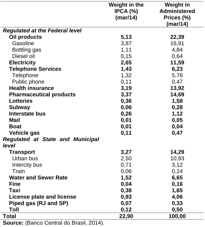
Table 2: Administered goods and services prices category, in the IPCA ... 12
SUMMARY
1 Introduction ... 10
2 Literature Review ... 15
2.1 Trend Inflation ... 16
2.2 Administered Price Sector ... 17
3 The Structural Model... 19
3.1 Household ... 19
3.2 Firms ... 21
3.3 Monetary Policy... 25
3.4 Price Dispersion ... 26
3.5 Price Adjustment Gap and Marginal Markup ... 28
3.6 The log-linearized model ... 29
4 Results ... 34
4.1 The Welfare-based Loss Function Under Trend Inflation ... 34
4.2 Optimal Policies ... 36
5 Conclusions ... 39
References ... 41
Appendix ... 44
Appendix A - Derivation of the optimal Pricing Rule ... 44
Appendix B – Complete non-linear model... 48
Appendix C – The Steady State model ... 50
Appendix D – Derivation of the price adjustment gap and marginal markup ... 52
Appendix E – Derivation of the Log-linear model model ... 55
Appendix F – Derivation of the Welfare-based Loss Function Under Trend Inflation ... 66
1 Introduction
Recent years in Brazil have seen the resurgence of the discussion about the use of administered prices 1 by the government as a way to hold back inflation, notwithstanding policies used by the monetary authority. Prices of goods and services can be divided in two groups, market prices that follow regular forces of supply and demand, and administered prices that are set and monitored by government or regulatory agencies.
The characteristics of each group cause prices to follow different paths, thus causing prices to disperse, i.e. to change their relative weight compared to the general price index. The nature of this dispersion and how this correlates to the optimal policies of the monetary authority are the purpose of this study. To accomplish this, we’ll work with a standard New Keynesian DSGE model of a closed economy with firms from two sectors, a continuum of firms in the free price sector and a single firm in the administered price sector.
In Brazil, since June 1999, the Monetary Policy Committee (Copom) of the Central Bank of Brazil (BCB) has adopted an inflation targeting mechanism as a framework to set monetary policy, by means of Brazilian Act 3.088. The National Monetary Council (CMN) annually sets the target and the tolerance range for the inflation index, for one and a half year ahead, and the Central Bank, with its monetary policies, seeks to maintain the inflation for the period in this range.
Since its inception, in only three years this goal was not achieved and the inflation, measured by the IPCA (Broad Consumer Price Index), closed the year above the upper limit of the tolerance interval set for the period. Table 1 shows the goals, tolerance intervals and inflation for the period, and marks the periods when the actual inflation exceeded the target and the tolerance.
1
Table 1: Inflation Targets history in Brazil from 1999 to 2016
Year Target
(%)
Tolerance Range (pp)
Effective inflation (IPCA)
1999 8 2 8,94
2000 6 2 5,97
2001 4 2 7,67
2002 3,5 2 12,53
2003 3,25 2 9,3
(a)
4 2,5
2004 3,75 2,5 7,60
(a)
5,5 2,5
2005 4,5 2,5 5,69
2006 4,5 2 3,14
2007 4,5 2 4,46
2008 4,5 2 5,90
2009 4,5 2 4,31
2010 4,5 2 5,91
2011 4,5 2 6,50
2012 4,5 2 5,84
2013 4,5 2 5,91
2014 4,5 2 6,41
2015 4,5 2 9,34(b)
2016 4,5 2 5,59(b)
Source: Central Bank of Brazil (BCB).
a) In an open Letter from 21.01.2003, the targets for 2003 and 2004 have been adjusted to 8.5% and 5.5% respectively.
b) Market expectation, from the medians of the top five institutions of the Focus report from 07.08.2015.
Experts consulted by the Central Bank, and published in the Focus Report, forecasts that the inflation this year will exceed the ceiling of the inflation target, set at 6.5%, a fact that happened the last time 10 years ago.
Table 2: Administered goods and services prices category, in the IPCA Weight in the
IPCA (%) (mar/14)
Weight in Administered
Prices (%) (mar/14) Regulated at the Federal level
Oil products 5,13 22,39
Gasoline 3,87 16,91
Bottling gas 1,11 4,84
Diesel oil 0,15 0,64
Electricity 2,65 11,59
Telephone Services 1,43 6,23
Telephone 1,32 5,76
Public phone 0,11 0,47
Health insurance 3,19 13,92
Pharmaceutical products 3,37 14,69
Lotteries 0,36 1,58
Subway 0,06 0,28
Interstate bus 0,26 1,12
Mail 0,01 0,05
Boat 0,01 0,04
Vehicle gas 0,11 0,47
Regulated at State and Municipal level
Transport 3,27 14,29
Urban bus 2,50 10,93
Intercity bus 0,71 3,12
Train 0,06 0,24
Water and Sewer Rate 1,52 6,65
Fine 0,04 0,16
Taxi 0,38 1,65
License plate and license 0,93 4,06
Piped gas (RJ and SP) 0,07 0,33
Toll 0,12 0,50
Total 22,90 100,00
Source: (Banco Central do Brasil, 2014).
This last characteristic2 makes them a source of inertial inflation, with less of an influence from current monetary policies, and due to its weight in the headline index, must be treated carefully while trying to reach inflation targets.
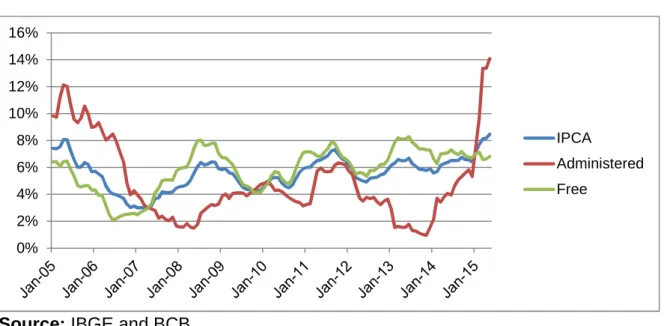
Comparing the full IPCA index with the administered and free prices category from the last 10 years, in Figure 1, it shows how controlling increases in administered prices can influence whether the IPCA will converge or not to the set target.
Figure 1: Annualized Change in full IPCA, Free and Monitored
Source: IBGE and BCB
It is easy to see that, in the last three years, at first the regulated prices inflation, well below the free prices inflation contributed to the IPCA to stay within the limits of the established goal, however, in a second stage, the need to readjust those prices causes the headline index to be, at present, well above the upper limit of the band.
This is a typical “dog with two owners” problem, where different agents, even when trying to reach the same goal, are not able to cope with the various influences that one’s action causes to the other, thus inflicting problems to the rest of the market.
This various characteristics of administered and free prices cause an increased dispersion between the prices in the economy thus provoking an adverse effect on the welfare of the population.
2
Dependency on international prices and larger pass-through coefficients per-se are not sources of inertial dynamics. However, there are some inertial characteristics observed in international prices and in the way domestic prices are complementary to import/export prices that might be passed into administered prices in general equilibrium.
0% 2% 4% 6% 8% 10% 12% 14% 16%
IPCA
Administered
The model’s results suggest that price movements in either sector will have impact on both sectors for two reasons. First, that price dispersion causes productivity to be lower. Since price dispersion is a change in the relative price of either sector, to general prices in the economy, when a move in the prices from one sector is not followed by the other, relative weights will change and will impact the productivity in both sectors.
Second, the path followed by the administered price sector is considered in the future inflation expectation, which is used by the firms in the free sector to adjust their optimal price. When this path leads to a higher inflation expectation, the firms in the free sector will choose a higher markup, to accommodate thie future expectation, thus leading to a higher the trend inflation, when there is an imperfect competition in the free sector.
2 Literature Review
Dynamic Stochastic General Equilibrium (DSGE) models have become an increasingly important tool for Central Banks around the world (Tovar, 2009) in the last twenty years. The list of Central Banks that are using and have published their work with DSGE models is increasing3, as is the literature about the topic.
As for the development of DSGE models, the New Keynesian Standard Model has become the “workhorse for the analysis of monetary policy, fluctuations, and welfare” (Galí, 2008). This model incorporates imperfect competition in the goods market (Blanchard, et al., 1987) and price rigidity, through a staggered price setting structure (Calvo, 1983), which sets it apart from the Classical Monetary Model.
One of the main characteristics of the standard NK model is what´s been called the “Divine Coincidence” (Blanchard, et al., 2005), that is, any monetary policy that will stabilize the inflation rate after a preference or technology shock, will also stabilize the output gap, when price stickiness is present. This property has called the attention of policy makers because, in reality, central banks perceive a trade-off between stabilizing inflation and output gap (Alves, 2014). One way for DSGE models to get rid of the Divine Coincidence, is using some tricks, such as staggered sticky wages, and so on.
Another point that has caught the attention of many (Alves, 2011), is the fact that these models, with partial indexation, often will set the optimal level of inflation at zero (Woodford, 2003) or negative (Friedman, 1969) levels, while Inflation Targets around the world are all set to much higher levels, as show in the Table 3.
3
Table 3: Inflation Targets examples
Country Inflation targeting adoption date
Inflation rate at adoption date
Target inflation rate
New Zealand 1990 3.3 1 – 3
Canada 1991 6.9 2 +/– 1
United Kingdom 1992 4.0 2 +/– 1
Sweden 1993 1.8 2 +/– 1
Australia 1993 2.0 2 – 3
Brazil 1999 3.3 4.5 +/– 2
Chile 1999 3.2 3 +/– 1
Source: (Roger, 2010)
Of course, Inflation Targets are not sure to be set to optimal welfare, because many other factors will take part when setting these targets (Alves, 2011), like political pressure, lobbies and even uncertainty about the model itself.
2.1 Trend Inflation
In contrast, some models that have a positive inflation target assume a total indexation of prices (in Calvo Prices, when firms are not optimizing their price), like in (Castro, et al., 2011) which will make prices to converge to a steady state when inflation is equal to the target, causing price dispersion to disappear in the long run.
Part of the discussion about a positive trend inflation in the steady state comes from the Zero Lower Bound Problem (Ascari, et al., 2014), that occurs when the short-term nominal interest rate is at or near zero, causing a liquidity trap and limiting the capacity that the central bank has to stimulate economic growth.
Another property of models using positive trend inflation in the steady state is shown by (Alves, 2014), that it causes the “Divine Coincidence” to disappear, forcing the monetary authority to choose between stabilizing inflation or the output gap. This happens when prices of non-optimizing firms are not fully indexed to trend inflation, or when inflation is not maintained at exactly zero.
Also, another contribution by (Alves, 2014) that will be used in this paper is the derivation of the welfare-based loss function under trend inflation (TIWeB), a second order (log) approximation of the loss function in the steady state with positive trend inflation. As shown by (Alves, 2011), when trend inflation departs from zero, in the positive side, the welfare function is much more concave, thus resulting in an underestimation of the welfare loss when the loss function is computed on the zero inflation steady state.
2.2 Administered Price Sector
Some authors4 when modeling the Brazilian economy in a DSGE model, won´t clearly define an administered sector, but consider the nature of the administered prices as part of the price rigidity created by Calvo pricing, since their focus is not on this dynamic between sectors.
The Central Bank of Brazil SAMBA (Stochastic Analytical Model with a Bayesian Approach) model (Castro, et al., 2011), although far more complex model than a New
Keynesian Basic Model, incorporates an administered prices as one type of
intermediate producers in the consumption goods sector. This producer will face almost the same challenges (cost minimization problem and downward-sloping demand curve) as the other producers in the consumption goods sector, except for the fact that the adjustment rule for the administered prices is not optimal. Also, it is composed by a fraction 1 − of all the firms j in the consumption goods sector,
given by , , and all firms faces imperfect competition, also with Calvo pricing
rules.
In (Vereda, et al., 2010) the model consider three subsector in the producers sector group, Tradables, Non-tradables and Administered, with each subsector being composed by a continuum 0,1 of firms, facing imperfect competition and Calvo type pricing mechanism.
Another paper (Freitas, et al., 2006) builds on a much simpler model, with firms from two sector, Administered and Non-Administered (free). Free prices sector is composed by a continuum 0,1 of firms, while the administered prices sector is composed by only one firm. Furthermore, firms in the free sector faces imperfect competition, with Calvo type prices, while the administered sector firm has only one price correction rule.
For the simplicity, we have chosen to work with a model close to (Freitas, et al., 2006), with the distinction of this being a closed economy, as opposed to an open economy in the text by the authors.
4
3 The Structural Model
The model developed in this paper is a standard New Keynesian Basic Model, as described by (Woodford, 2003) and (Galí, 2008), incorporates imperfect competition in the goods market (Blanchard, et al., 1987) and price rigidity, through a staggered price setting structure (Calvo, 1983). The model contains two sectors, for free and administered price firms, in the same way as in (Freitas, et al., 2006).
Also, the model has positive trend inflation in the steady state, following (Ascari, et al., 2014), resulting in the Generalized New Keynesian Phillips Curve (GNKPC), a name coined by the authors. Furthermore the welfare analysis is based on the derivation of the Trend inflation Welfare-Based loss function, as derived by (Alves, 2014).
As will be further explained in the following sections, the model is composed by an infinitely-living household that supplies labor to both administered and free price sector firms, and consumes an aggregate bundle of all firms. Firms transforms labor into final products, subject only to technology constrains, and pay wages to the household.
3.1 Household
The household in this economy will maximize its intertemporal discounted utility function by solving the following problem
,, ,, , ∑!" , (1)
s.t.
Where + is the subject discount factor, ,-, and , , are prices of goods from the free and administered sector, respectively. .-, and . , , are the quantities of free and administered sector goods consumed. / is the price of a bond in t, with maturity in t+1, that solves / = 1 + 1 ' . 1 is the nominal interest rate in t. 2 is the quantity of bonds in period t. 3 is the nominal wage, and 4is the hours of work in the period. Finally, 5 is the lump-sum tax and dividends.
The utility function is a constant relative risk aversion (CRRA), given by
, = ('8(78− 9 (<;(:; (3)
Where =' is the intertemporal elasticity of substitution, >' is the Frisch elasticity of labor supply and 9 is a labor supply shock. Since total labor suplied is given by
= , + , (4)
Maximizing the household intertemporal discounted utility function will result in the following optimal labor supply and Euler equation
)
# =
) ,
# =
) ,
# = − ?,@, = 9
; 8 (5)
(
8= AB##:(C ( + D E ( :(
8 FG (6)
Since working in both sectors are perfectly substitutes, there will be wage equalization in the model.
Consumption of goods from the free sector firms is given by a Dixit-Stiglitz aggregator, as is the price index from free sector
, = H I, ,
J7( J KI
( LJ7(J
(7)
# , = H #( I, , ('JKIL (
Where M > 1 represents the elasticity of substitution between goods. To find the solution for the household intertemporal problem, we must first define the consumption bundle aggregator, from the goods of the free and administered sector
= O, (7O,
OO ('O(7O (9)
Where P ∈ 0,1 is the participation of the free sector goods in the consumption bundle. Maximizing the Consumption function (9) for .-, and . , , subject to an budget constraint function for the period
# , , + # , , ≤
When R = . ,, we find the demand for the goods of each sector as
, = O B##,C '(
(10)
, = ( − O B##,C'( (11)
When substituting (10) and (11) in (9), we find the price index for period t
# = #O, # ,
('O (12)
Following this, when prices are equal the contribution to the price index will be P e 1 − P, and the demand for each firm z will be given by
I, , = E##I, ,, F 'J
, = O B##,C '(
E#I, , # , F
'J
(13)
3.2 Firms
Firms in the free price sector will use labor and technology to produce differentiated goods accordingly to the function
Aggregating labor as
, ('T = U I, , ('T KI
(
We get the aggregate production function for the free price sector
S , = , , ('T (15)
And for the administered price sector
S , = , , ('T (16)
Where AW,X and AY,X are exogenous process for technology levels in each sector, that we will assume to be stationary, and 0 < αW, αY < 1.
As per the market clearing condition, where = . , the demand for each z firm of the free sector, the firms demand of each sector and the aggregate production are set at
SI, , = E##I, ,, F 'J
S , (17)
S , = H SI, , J7(
J KI
( LJ7(J
(18)
S , = O B##,C'(S (19)
S , = ( − O B##,C '(
S (20)
S = SO, S(7O,
OO ('O(7O (21)
In the free sector firms will follow a Calvo pricing mechanism, in which firms will optimally readjust their price with a probability 1 − \ to ,],-, = ,],-,∗ , while with a probability \, firms will readjust their price accordingly to the rule
#I, , = #I, , '(_ '(` (22)
Where a = bc
bc7d and e- ∈ 0,1 is the level of indexation of the free sector (Christiano, et al., 2005). For the optimizing firms, when adjusting its price, firms will seek to maximize the expected profit, since they do not know when they will adjust their prices again, so this problem becomes
#I, ,∗ ∑ f!g" , <ghgi
#I, ,∗ j`7(, :g7(
# , :g SI, , <g− ) , :g
#:g E SI, , :g
, :gF ( (7T
k (23)
s.t.
SI, , <g= l#I, ,
∗ j
7(, :g7( `
# , :g m
'J
S , <g (24)
Where n , < ≡ + ppc:q
r is the stochastic discount factor, with s < as the marginal utility of consumption in t + . And Π , < is the accumulated gross inflation between periods t and t+j
Π , < = v
1 , wxy = 0 ,<
, z,,<{< z … z ,<
,< ' , wxy ≥ 1
First order condition is than given by
~ hgf , <g !
g"
v ( − J •#I, ,∗ €'J•j '(, <g'( `
# , <g ‚ ('J
S , <g
+( − T •#J I, ,∗ €
'J'(<T ('T )<g
# <g ƒ S , <g
, <g„ ( ('T
•j'(, <g'( `
# , <g ‚ 'J ('T
… =
So, following (Ascari, et al., 2014b), we can write
•†I, ,∗ €(<(7TJT = J J'( ('T
‡
ˆ (26)
Where relative optimal prices are E‰],-,∗ = bŠ,‹,c ∗
b‹,cF , net inflation in the free sector is
Ea-, =bb‹,c7d‹,c F , and Œ• = 3 ,Ž • is the real wage. By using the definition of the
stochastic discount factor Bn, < ≡ + pc:q
pr C , and the fact that Bs < = •‘ •’c= .<
'“C
( '“< , in equilibrium), ancillary variables ” and • can be written in a recursive way
‡ = S'8S ,
( (7T
, 7(
(7T – + h —(7T7` J ƒ_ , <(
J
(7T ‡
<(„ (27)
ˆ = S'8S , + h —` ('J ˜_ , <(
J'( ˆ<(™ (28)
Also, from (7), and considering that š t ⊂ 0,1 are the firms not optimizing their prices in t, free sector prices will evolve according to
# , = Hh_` ('J'( •# , '(€('J+ ( − h •#I, ,∗ €('JL ( (7J
(29)
Or, dividing by ,-,
( = h_` ('J'( _ ,J'(+ ( − h •† I, ,
∗ €('J (30)
The Administered Price Sector Firm
For the firm in the administered sector, price definition will follow the rule
Where a = bc
bc7d is the net inflation, and e ∈ 0,1 is the level of indexation of the administered prices to past inflation a' or to the inflation target a• . Dividing by ,, '
_ , = _'(` _œ ('` (32)
Aggregate Inflation
From (12), = ,-,ž , ,'ž , divided by ,'
_ = _O, _ ,
('O (33)
Considering the inflation from each sector
a-, = Ÿ\a' '‹ '¡ H1 − 1 − \ •‰],-,∗ € '¡L¢¡'
a , = a ' £a¤ ' £
So (12) can be rewritten as
_ = Ÿh_'` ('J'( H( − ( − h •†I, ,∗ €('JL¢J7(O ˜_
'(` _¥ ('` ™('O or
( = Ÿh_'` ('J'( H( − ( − h •†I, ,∗ €('JL¢J'(O ˜_
'(` _¥ ('` ™('O_ '(
(34)
3.3 Monetary Policy
B(<D(<¦̅C = B__œCˆ_BSSœCˆS¨© (35)
Where a• is the inflation target and also the trend inflation in the steady state.
3.4 Price Dispersion
From the production equations (14 to 16) labor demand can be derived. Also, using the equations for the demand in each sector (11 and 13), and considering that in equilibrium .ª, = ª, , labor demand can be rewritten as
, = ES,F ( (7T
B# , O# C
7(
(7T E#I, , # , F
7J (7T
KI (
(36)
, = ES,F ( (7T
H # , ('O # L
7( (7T
(37)
Where bžb‹,c
c is the relative weight of free goods prices in the general price index, EbŠ,‹,c
b‹,cF '¡
is the dispersion of prices among free goods firms and b£,c
'ž bc is the relative weight of the administered prices in the general price index of the economy.
For simplicity, we can consider that «-, = « , = « and ¬- = ¬ = ¬, and following the aggregation equation for labor (4), we have
= BSC ( (7TB# ,
O# C 7(
(7T E#I, , # , F
7J (7T
KI
( + BSC(7T( H # ,
('O #L 7( (7T
= BSC ( (7T-B# ,
O# C 7(
(7T E#I, , # , F
7J (7T
KI
( + H # ,
('O #L 7( (7T®
(38)
So
¯ , = B#O#,C 7(
(7T E#I, , # , F
7J (7T
KI
¯ , = H('O ## , L 7( (7T
(40)
And
¯ = ¯ , + ¯ , = B#O#,C 7(
(7T E#I, , # , F
7J (7T
KI
( + H # ,
('O #L 7(
(7T (41)
Where š is the total price dispersion for this economy. As it is shown, the total price dispersion, for both the sectors of free goods, of administered goods and the general economy, is affected not only by the level of sectorial prices, but also by the relation of each sectorial prices with the general price level of the economy. This means that for the total price dispersion not to affect labor productivity, it is necessary that all prices maintain its relative weight (,],-, = ,-, ; ,-, = P, ; ,, = 1 − P , .
This means that in an economy with positive inflation all prices should be adjusted equally, which is part of the objective of having an inflation target system. When prices are adjusted outside this rule, either by the free or the administered price sector, there will be dispersion in both sectors, because in either case it will affect the general price index, thus causing both sectors prices to be in discrepancy to their relative weight.
So, an administered price adjustment policy that does not fall in line with the adjustments in the free goods sector prices will cause price dispersion.
Equations (39) and (40) can also be written as to show their law of motion
¯ , = B_O,C 7(
(7T ( − h •† I, ,
∗ €(7T7J + h B_ , O_C
7( (7T _
'( 7J`
(7T _ , (7TJ ¯ , '( (42)
¯ , = A_7(` _¥ (7`
_ G
7( (7T
¯ , '( (43)
dispersion, real wage will fall (Alves, 2014), since from equation (5), the fall in the consumption, more than compensates the rise in employment.
It´s also important to note that one component of this price dispersion comes from relatives aggregate prices, from each sector and the general price index, which means that a shock in the administered sector will cause the dispersion to affect the marginal cost in the free sector.
Also, the price dispersion is dependent from the trend inflation level and how prices in each sector adjust to past inflation, i.e. the indexation parameters.
3.5 Price Adjustment Gap and Marginal Markup
As shown by (Ascari, et al., 2014) from equations (26), (27) and (28), is possible to arrive in the following equation for the optimal price
†I,∗ = •J'(J l('h _
` (7J :J7(
('h _J7` J(7T m ± ‚ (7T (:T J7(
(44)
Assuming linear production ¬- = 0 , we have the relation between optimal price and marginal cost of the free sector
†I,∗
± = J'(J B('h _
` (7J :J7(
('h _J7` J C (45)
Assuming no indexation e- = 0 and, with equation (30), is possible to rewrite as
²- =³’‹ = EbbŠ,‹∗‹F B´Š,‹ ∗
³’‹C = H
'µ¶·7d
'µ L
7d d7·
H¡'¡ B 'µ¸¶'µ¸¶·7d· CL (46)
Where the first term is the Price Adjustment Gap and the second term is the Marginal
that, now, the inflation a is also dependent on the inflation of the administered prices sector.
As discussed by the authors, the first term decreases with inflation, since this relation is the inverse of the optimal price to aggregate free sector prices. As inflation increases, so does the gap between firms optimizing their prices and those that optimized in the past, considering that e- = 0 and there is no indexation to past inflation.
The second term will increase with inflation, and the newly optimized prices will be set further from the average price of the free sector. This is because of the highly forward-looking behavior of the firms in the free sector. The overall effect will be dependent on the elasticity of demand M.
In this case, since inflation is also dependent on the inflation of the administered price sector, we can see that a rule for adjusting prices in the administered sector will have an impact in both sectors.
3.6 The log-linearized model
For any ℵ , variable, the notation ℵº ≡ log ℵ ℵœ⁄ is its deviation in log of its value in Steady-State ℵœ with inflation greater than zero (Trend StSt).
From the Euler equation
Sº = Sº<(− 8'( ¦¿ − _¿<( (47)
From the labor supply equation
–¿ = ;º + 8º (48)
From the labor demand equation
Price dispersion equations
¯º , = ƒ( − h O_œ` '( ('J
('T „ ƒ−J†¿I, ,∗ − _¿ ,
( − T „
+ hO('T( _J ('`('T ƒ J − ( _¿ , + _¿ − J` _¿'(
( − T + ¯º , '(„
(50)
¯º , =('T` _¿ − _¿'( + ¯º , '( (51)
Taylor rule
¦̂ = ˆ__¿ + ˆSSº + © (52)
The General New Keynesian Phillips Curve (GNKPC)
The log-linear version of the GNKPC is obtained by the derivation of the equations (34), (26), (27) and (28)
aÁ =P˜1 − •e- 1 − M €aÁ\a ‹ '¡ <¡'' ™˜1 − •1 − \aM − 1 P + e − Pe‹ '¡ <¡' € 1 − M ‰̂],-,∗ ™
− M − 1 P + e − Pe +P P + e − Pe1 − P e aÁ '
(53)
B( +('TJT C †¿I, ,∗ = ‡º − ˆº (54)
‡º = –¿ − 8Sº +•Sº ,'º ,€
('T + h _
J•(7` €
(7T H8Sº − –¿ +•º ,'Sº ,'` J_¿ €
('T + B
J_¿ , :(
('T + ༠<(CL (55)
ˆº = Sº , − 8Sº + h _` ('J <J'(•8Sº − Sº , + ` ( − J _¿ + ˜ J − ( _¿ , <(+
The General New Keynesian Phillips Curve (GNKPC) in terms of Output gap
Another way to write the GNKPC, which is useful for our purpose of deriving optimal policies, is to write it in terms of the output gap as the only demand variable. From equations (42), (43) and (44), and considering these other ways of writing †¿I, ,∗ and
Sº ,
†¿I, ,∗ = h_` (7J :J7(
('h_` (7J :J7(•_¿ , − ` _¿'(€ (57)
Sº , = Sº + #º − #º , = Sº + Â , (58)
Where
The GNKPC can be written as
;• hà − (€ ÄO (
('Thà J − ( + `
( − T Å _¿
= H ( − hœ 8 − ( + •( − hÀ( − TL Æ¿;
+ A•( − hÀ E( − TF − ( − h( œ G ,
+ v;•( − hÀ vAh O_œ` '( ('J('T− (G l JÃhœ ( − hœm +
O('T( hÃJ ( − T …
− ( + JÃT ( − hœ… Çhœ _,
+ ;•( − hÀ vAh O_œ` '( ('T('J− (G E (
( − TF −O ( ('ThÃ
( − T… _¿ , −( − T _¿` '(
+ ;•( − hÀ AO('T( hïº , '(+ ¯º , '(G
+ -hœ ƒ ( + JÃT ( − hœ + ( − J „ + hhœ à J( − T® Ç_, <(+ È •º€
+ •hà − hœ€ ‡º<(
(59)
Where
”É = ˜1 − +\Ù A>•šÊ-, + šÊ , € + E> + 11 − ¬F zÁ + E> + 11 − ¬F E¬ + > + = 1 − ¬ − 1F «> + 1 Ê
+ E1 − ¬F Μ1 -, G + +\à HÌ ”É < +1 − ¬ ÌM ¶, < L
² •«Ê€ = - 1 − +\̅ ƒ¬ + > + = 1 − ¬ „ + •1 − +\= − 1 > + 1 À >1 − ¬ AE¬ + > + = 1 − ¬ − 1FG® «> + 1 Ê
+\̅ = \+a ‹ '¡ <¡'
+\Ã = \+a¡ ' 'Í‹
1 + Mì = B1 +1 − ¬CM¬
If we consider that e- = ¬ = 0 , meaning that there is no indexation in the free sector and constant return on labor, we get
; \+a¡− ( O\a¡ J − ( + ` _¿
= ( − hœ 8 − ( + ( − \+a¡ ; Æ¿ + ( − \+a¡ − ( − \+a¡' Â
,
+ -; ( − \+a¡ - h O_œ'( ('J− ( l M\+a¡'
( − \+a¡' m + O\a¡ J − ( + (®
−( − \a\a¡'¡' ® _¿ , − ` _¿'(+ ; ( − \+a¡ ˜O\a¡¯º
, '(+ ¯º , '(™
+ -\a¡' ƒ \a¡'
( − \a¡' + ( − J „ + \a¡J® _¿ , <(+ È •º€ + \a¡ − \a¡' ‡º
<(
(60)
Which means that, if also set e = 0 , past inflation will only come from price dispersion in the free sector, which will be given by
¯º , '(= - h O_œ'( ('J− ( l J\a ¡'
4 Results
4.1 The Welfare-based Loss Function Under Trend Inflation
Following (Alves, 2014) I derive the Welfare-based Loss Function Under Trend Inflation (TIWeB) for this economy. The TIWeB is derived from a second-order approximation of the (negative) true welfare function, around the steady state with trend inflation, as denoted by the author.
First step of this process is to transform the aggregate disutility function as a function of only aggregate variables. This is important because with trend inflation, in the case where indexation of the free sector is not full e- ≠ 1 , for the firms not optimizing prices in period t, it means that prices of each firm Ð will not converge to a single
steady state price, so there will be dispersion in the steady state.
Consider that
©Ñ = (<;9 BS C (:; (7TÒ
(61)
Ó = S('8(78 (62)
Ò = -B# , O# C 7( (7T-h_ '( 7J` (7T_ , J (7TÔ , '( 7J
(7T+ ( − h H J
J'( ('T ‡ˆL 7J
(7T (7J® + H # , ('O #L
7( (7T®(<;
(63)
Ô(7T7J, = ( − h H J
J'( ('T ‡ˆL 7J
(7T (7J + h_ '( 7J` (7T_ , J (7TÔ , '( 7J (7T (64)
Where ©Ñ is the average desutility function, Ó is the utility function, Ò is a measure
of the aggregate relative prices, and Ô , is a measure of the aggregate relative
Welfare Õ is computed as a discounted flow of preferences in equilibrium, and it evolves according to a Bellman equation
Ö = Ó − ©Ñ + Ö<( (65)
So, following (Alves, 2014b), we arrive to
Ö = −(Îל ∑! Ø
Ø" Ùœ <Ø+ ¦†••••ÖÖ (66)
And
Ùœ = •Ç_, − Ú¥h€Î+ Û ˜Â , + ( − T ™Î+ Û ˜Â , + ( − T ™Î+ EÛÜÒÆF Æ¿ + ÝÖ Î
(67)
Where
ÞOJJÃhÕhÃ'(€•(' hÀ = ÛÒ
Ýß; ('8 '8'T(<; = ÝÖ
; ('8 '8'T
Î (<; = ÜÆ ';Î'TÎ'Î;
('T (<; = Üß ÞO
ÛÒ ('TÎ = Û
àO
ÛÒ ('TÎ = Û
#º − #º , = Â ,
#º − #º , = Â , Úh
JÃhÕhÃ'(€= Ú¥h
hà − á•hà − (€ B( +(ÎJà − (
ÎJÃhÃC = Úh
O(7T( Ä ('h B (7hœ (7hC
7JÃ (7J
('h_J•(7` €(7T Å = ÞO
( − O (7T( = àO
( + ; '(ÞO+ ( + ; '(à
O = â hœ
('hœ= á
Ç_, = _¿ , − ` _¿ '(
The derivation of the TIWeB loss function is detailed in the appendix.
4.2 Optimal Policies
As of the discussion by (Alves, 2014), the rules (Discretion and Unconditional Commitment) are derived bellow. Central bank will implement inflation targeting by keeping the unconditional mean of the inflation rate a• at the center, which means Ìa = a•, and also means that ÌaÁ = 0.
In all cases, as stated by (Alves, 2014), the Central Bank will minimizes the Lagrangian problem formed by the discounted sum of the derived Loss Function, subject to the IS, the GNKPC curves and to ÌaÁ = 0.
For the policy under discretion, as argued by (Alves, 2014), we’ll assume that the Ergodic Theorem holds, and so Ì 1 − + ∑!ã" +ãaÁã< = 0 is a good approximation of ÌaÁ = 0.
Optimal policy under unconditionally commitment
Optimal policies under commitment means that the monetary authority will seek to minimize the loss function, while being able to commit, with full credibility, to a policy plan (Galí, 2008). In this case, the optimal policy under unconditionally commitment is the one derived by (Damjanovic, et al., 2008), that also appears in (Alves, 2014).
As shown in the appendix, the result is
−ΕÇ_, '(€` + Hä` + ( − TL Æ¿` 'Î
+ Ÿå` − æ@Î J − ( +( − T + − ¢ Æ¿` '(
+ Hç` − è@Î J − ( − ( − T + @` éL Æ¿ + ê Æ¿<( ` =
H\ Pa• ‹' d7ëd7· − 1L = @(
žd7ëd µÃ
'Í = @Î ¡Ãµœ
'µœ = @ì
\̅ H 1 + Mì 'µœµœ + 1 − M L + \à 'Í¡ = @í
Ÿ>•1 − +\Àîï ïð+ ï{Mñ − 1 +
Mì 'µœµœ ¢ = @ò
>•+\Ã − 1€ Hï{ M − 1 + £
'ÍL = @é
{EõöóôF• '¸µÃ÷7d€
ŸH• '¸µœ€ “' <• '¸µÃ€d7ëø L• '¸µÃ€'•µÃ'µœ€¸• '¸µÃ€Bø:dd7ëC¢=
•µÃ'µœ€¸ • '¸µÃ€ =
ù• '¸µÃ€žd7ëd µÃ l 'žd7ëd µÃ÷m =
• '¸µÃ€ù÷ l 'žd7ëd µÃ÷m= ú
>•1 − +\À = •1 − +\À> =
æ ï ïð+ ï{M = ä
è ï ïð+ ï{M + ïû = å
+ïü= ç
+\Ã 'Í¡ = ê
Optimal policy under discretion
Optimal policy under discretion means that the monetary authority will seek to minimize the Lagrangian problem taking into account only the contemporaneous variables (Alves, 2014). It means that the Central Bank will treat the problem as a series of optimization problem, making whatever is the optimal decision in each period (Galí, 2008).
−Î` ý•_¿ , − ` _¿ '(€ − Î ` •_¿ , <(− ` _¿ € + þ Æ¿ î@é+ ` @ ñ
+ A þ B` @ò+( − TC − )` ( − T − )O` (
('Thà J − ( @ÎG Æ¿<( =
Where
2 E ª
ΕöF
5 Conclusions
In (Ackley, 1959) there was already a discussion about the concept of "administered prices" and the controversy about their responsibility for movements of the general price level, which shows the importance and longevity of this theme.
In this work we have developed a DSGE model with two sectors, for administered and free prices, with positive trend inflation in the steady state. The objective was to show how an adjustment rule for the administered prices could impact the whole economy, and, also, what the optimal policies should be concerning the welfare of the households.
This work has expanded previous works on two fronts, by incorporating trend inflation in the steady state, and by having two sectors in the economy. The literature about administered prices in a DSGE model is not very extensive, with this being more a characteristic of the model, than an objective of study. In the case of the study by (Freitas, et al., 2006), we have come to a close conclusion with the loss function, even if the authors uses a different approach.
We have shown the crucial role played by price dispersion in this model. With only one sector, and with the trend inflation in the steady state, price dispersion will appear when the non-optimizing firms are not able to adjust their price according to past inflation, i.e. with indexation less than one.
In our case, besides the same issue, there is also a price dispersion between the aggregate free sector prices and the general price index, and respectively, between the aggregate administered price sector and the general price index. But since the general price index is a composition of the two sectors, a distortion in any sector will cause the price dispersion in both sectors.
setting the interest rates, if other authorities are pushing the administered prices in some other direction, to accommodate other objectives, there will be a loss of welfare affecting the whole economy.
Also, we show that when administered prices don´t follow a predictable path, firms of the free sector will have difficulty in setting their optimal price when it can adjust. This means that these firms will set a higher markup in other to accommodate the expected inflation, pushing for a higher inflation and a higher price dispersion in the free sector.
Finally, we show how relative prices in both sectors will affect the welfare, being part of the derived loss function, a result that is in line with (Freitas, et al., 2006). Also, the backward looking nature of the administered price sector will cause the optimal policy under commitment, to look further to lagged terms.
Although our model uses a very simple rule for the administered price sector, in reality each industry in the sector will have a specific rule that will mostly account for: past inflation, exchange rates movements and productivity. Also, while not officially, other authorities (federal, state and municipal government, and some public authorities) have the power to impose timely adjustment to those prices as well.
Recent times have seen how an attempt to impose a specific agenda over the administered prices can backfire, creating in the medium and long run, an increased difficulty to the Central Bank to accommodate all price movement and follow the defined inflation target. Figure 1 shows how these price movements have evolved in the past ten years, and that inflation in both sectors have hardly been the same.
References
Ackley, Gardner. 1959. Administered Prices and the Inflationary Process. The American Economic Review. No. 2, 1959, Vol. Vol. 49.
Alves, Sergio Afonso Lago. 2014. Lack of Divine Coincidence in New Keynesian
models. Journal of Monetary Economics. 67, 2014.
—. 2014b. Online Appendix to Lack of Divine Coincidence in New Keynesian
Models. ScienceDirect. [Online] 07 02, 2014b. [Cited: 06 22, 2015.] http://dx.doi.org/10.1016/j.jmoneco.2014.07.002.
—. 2011. Optimal Policy When the Inflation Target is not Optimal. LACEA LAMES - Annual Meeting of the Latin American and Caribbean Economic Association | Latin American Meeting of the Econometric Society . Santiago, Chile : s.n., 2011.
Aoki, Kosuke. 2001. Optimal Monetary Policy Responses To Relative-Price
Changes. Journal of Monetary Economics. 48, 2001.
Ascari, Guido and Sbordone, Argia M. 2014b. Appendix to The Macroeconomics
of Trend In‡ation. Journal of Economic Literature. 2014b.
—. 2014. The Macroeconomics of Trend Inflation. Journal of Economic Literature.
2014.
Banco Central do Brasil. 2014. Preços Administrados - Serie Perguntas Mais Frequentes. 2014.
Blanchard, Olivier and Galí, Jordi. 2005. Real Wage Rigidities and the New
Keynesian Model. NBER Working Paper No. 11806. Cambridge, MA : National Bureau of Economic Research, 2005.
Blanchard, Olivier Jean and Kiyotaki, Nobuhiro. 1987. Monopolistic Competition
Calvo, Guillermo A. 1983. Staggered Prices In a Utility-Maximizing Framework. Journal of Monetary Economics. 1983, Elsevier Science Publishers B.V.
Carvalho, Fabia A. de and Valli, Marcos. 2011. Fiscal Policy in Brazil through the
Lens of an Estimated DSGE model. 32nd Meeting of the Brazilian Econometric
Society. Salvador : s.n., 2011.
Castro, Marcos R. de, et al. 2011. SAMBA: Stochastic Analytical Model with a Bayesian Approach. Brasília : Banco Central do Brasil, 2011.
Cavalcanti, Marco A. F. H. and Vereda, Luciano. 2014. Multiplicadores dos gastos
públicos em um modelo DSGE para o Brasil. DSGE Models for Brazil: SAMBA and
beyond - Conference. São Paulo : FGV/EESP, 2014.
Christiano, Lawrence J., Eichenbaum, Martin and Evans, Charles L. 2005.
Nominal Rigidities and the Dynamic Effects of a Shock to Monetary Policy. Journal of
Political Economy. 2005, Vols. Vol. 113, No. 1.
Coibion, Olivier and Gorodnichenko, Yuriy. 2008. Monetary Policy, Trend Inflation
and the Great Moderation: An Alternative Interpretation. NBER Working Paper
Series. Cambridge, MA : National Bureau of Economic Research, 2008. Working
Paper 14621.
Damjanovic, Tatiana, Damjanovic, Vladislav and Nolan, Charles. 2008.
Unconditionally optimal monetary policy. Journal of Monetary Economics. 55, 2008.
Freitas, Paulo Springer de and Bugarin, Mirta Noemi Sataka. 2006. A Study On
Administered Prices And Optimal Monetary Policy: The Brazilian Case. LAMES -
Theoretical and Applied Economics. Mexico City : s.n., 2006.
Friedman, Milton. 1969. Optimum Quantity of Money and Other Essays. Brunswick,
New Jersey : Transaction Publishers, 1969. ISBN 978-1-4128-0477-6.
Galí, Jordi. 2008. Monetary policy, inflation, and the business cycle : an introduction to the New Keynesian framework. New Jersey : Princeton University Press, 2008.
Kanczuk, Fabio. 2014. Brazil Through the Eyes of CHORINHO. DSGE Models for Brazil: SAMBA and beyond - Conference. São Paulo : FGV/EESP, 2014.
Minella, André, et al. 2003. Inflation targeting in Brazil: constructing credibility under
exchange rate volatility. Journal of International Money and Finance. 2003.
Roger, Scott. 2010. Inflation Targeting Turns 20. Finance & Development. 2010. Tovar, Camilo E. 2009. DSGE Models and Central Banks. Economics: The Open-Access, Open-Assessment E-Journal. 2009, Vols. Vol. 3, 2009-16, Bank for
International Settlements.
Vereda, Luciano and Cavalcanti, Marco A. F. H. 2010. Modelo Dinâmico
Estocástico de Equilíbrio GeraL (DSGE) Para a Economia Brasileira: Versão 1.
Texto para Discussão No 1479. Brasília : IPEA Instituto de Pesquisa Econômica
Aplicada, 2010.
Woodford, Michael. 2003. Interest and Prices: Foundation of a Theory of Monetary Policy. Princeton, New Jersey : Princeton University Press, 2003. ISBN
Appendix
Appendix A - Derivation of the optimal Pricing Rule
Price definition (From Calvo (1983) e Yun (1996))
1 − \ of firms will optimize their price in period t •,],-,∗ €
\ of firms will adjust their price in period in t with the rule:
#I, , = #I, , '(_ '(` (A.1)
Where a = bc
bc7d , and e- ∈ 0,1 is the indexation level (Christiano et al. (2005)).
When adjust its price, firms seek to maximize the expected profit, since they do not know when they will adjust their prices again. This problem becomes:
#I, ,∗ ∑ f!g" , <ghgi
#I, ,∗ j`7(, :g7(
# , :g SI, , <g−
) , :g
#:g E
SI, , :g , :gF
( (7T
k (A.2)
S.t.
SI, , <g= l#I, ,
∗ j
7(, :g7( `
# , :g m
'J
S , <g (A.3)
Where n, < ≡ + ppc:q
r is the stochastic discount factor, and s < is the marginal utility
of consumption in t + . And Π , < is the accumulated inflation between the periods t and t+j.
Π , < = v
1 , ‰ y = 0 ,<
, z,,<{< z … z
,<
,< ' , ‰ y ≥1
~ hgf , <g !
g"
v ( − J •#I, ,∗ €'J•j '(, <g'( `
# , <g ‚ ('J
S , <g
+( − T •#J I, ,∗ €
'J'(<T ('T )<g
# <g ƒ S , <g
, <g„ ( ('T
•j'(, <g'( `
# , <g ‚ 'J ('T
… =
(A.4)
Where:
•,],-,∗ € < ¡Í'Í‹‹ = M
M − 11 − ¬1
-Ì ∑ \ n , < 3, < < A
-, <
«-, < G 'Í‹ƒΠ ' , < '
‹
,-, < „ '¡ 'Í‹
! "
Ì ∑ \ n , < ƒΠ ' , < '
‹
,-, < „ '¡
-, < !
"
Considering that 1 + ¡Í'Í‹
‹ = 1 − M +
¡
'Í‹ , and dividing both sides by,-, :
E#I, ,∗
# , F
(<(7TJT
= J'( ('TJ ∑ h
gf, :g) :g # :gƒS , :g, :g„
( (7T
•j 7(, :g7(
` j , , :g ‚
7J (7T g
∑ hgf, :g•j 7(, :g7( `
j , , :g ‚ (7J
S , :g g
(A.5)
From # , = H #( I, , ('JKIL
(
(7J and considering that š t ⊂ 0,1 are firms that
re-adjust price according to the rule of thumb in t, we have the equation of evolution of market prices:
,-, = H a '‹ '¡ ,],-, ' '¡ 1 + 1 − \ •,],-,∗ € '¡L
d d7·
# , = Hh_` ('J'( •# , '(€('J+ ( − h •#I, ,∗ €('JL
( (7J
(A.6)
Dividing by ,-, , and considering that a-, =bb‹,c
‹,c7d and that relative prices ‰],-,
∗ = bŠ,‹,c∗
b‹,c
, we have:
a-, = Ÿ\a' '‹ '¡ H1 − 1 − \ •‰],-,∗ € '¡L¢
d ·7d
Or,
†I, ,∗ = ƒ('h_` (7J7( _ , J7(
('h „
( (7J
(A.8)
Solving the optimal price equation recursively
First we rewrite the equation (A.5) as follows:
•†I, ,∗ €(<(7TJT = J
J'( ('T ‡
ˆ (A.9)
Whereas the real wage in the free sector is given by • = 3 ,Ž , using the discount
factor setting n, < ≡ + ppc:q
r , and the fact that s < =
•‘
•’c= . <
'“ ( <
'“, in equilibrium),
the ancillary ” and • are:
‡ = ∑ h gS
<g '8S , <g ( (7T , <g 7( (7T –
<gƒj7(, :g7(
`
j , , :g „ 7J (7T
!
g" (A.10)
ˆ = ∑ h gS
<g '8S
, <gƒj7(, :g7(
`
j , , :g „
('J !
g" (A.11)
Writing the two equations recursively:
‡ = S'8S ,
( (7T
,
7(
(7T – + h —(7T7` J ƒ_
, <(
J (7T ‡
<(„ (A.12)
ˆ = S'8S
Setting a Marginal Cost for the free price sector
± , = ('T( , ( T 7(–
,S , T
Appendix B – Complete non-linear model
Whereas . = , the complete system of nonlinear equations, is given by::
= ‹,c £,cd7
ž 'žd7 (B.1)
-, = P Bbb‹,cc C '
(B.2)
, = 1 − P Bbb£,cc C '
(B.3)
, = ,-,ž , ,'ž (B.4)
• = 4ù. “ (B.5)
c = +Ì AB
<c
¶c:dC Bc:dCG (B.6)
‰],-,∗ = ƒ 'µ¶c7d
‹ d7·¶‹,c·7d
'µ „
d d7·
(B.7)
•‰],-,∗ € <d7ë‹·ë‹ = ¡ ¡' 'Í‹
c
c (B.8)
” = '“
-,
d d7ë‹«
-,
7d
d7ë‹• + \+π7 ‹·d7ë‹Ì ƒa
-, <
· d7ë‹”
< „ (B.9)
• = '“ -, + \+π ‹ '¡ Ì ˜a
-, <¡' • < ™ (B.10)
, , = ,, ' a ' £a¤ ' £ (B.11)
a = Ÿ\a' '‹ '¡ H1 − 1 − \ •‰
],-,∗ € '¡L¢ ž ¡' ˜a
' £a¤ ' £™ 'ž
a ¡'ž = \a' ‹ ¡' < £¡'ž 'ž a¤ ' £ ¡'ž 'ž H1 − 1 − \ •‰
],-,∗ € '¡L
4 = E c
‹,cF d d7ë‹š
-, + E £c,cF d d7룚
, (B.13)
š-, = B¶ž‹,cC 7d
d7ë‹ 1 − \ •‰
]∗,-, € 7·
d7ë‹+ \ B¶‹,c ž¶cC
7d d7ë‹a
' 7· ‹
d7ë‹a-, d7ë‹· š-, ' (B.14)
š , = A¶c7d £¶¶¥ccd7 £G 7d d7룚
, ' (B.15)
B <c < ̅C = B
¶c
Appendix C – The Steady State model
Whereas _œ is the inflation in the SS and the Goal of inflation, and that in SS:
_œ = _ = _
S =OOSO('OS(7O(7O (C.1)
S = OS (C.2)
S = ( − O S (C.3)
– = 9 ;S8 (C.4)
_œ = ( + D (C.5)
†I∗, = H('h_œ` (7J :J7(
('h L
( (7J
(C.6)
•†I∗, €(<(7TJT = J
J'( ('T ‡
ˆ (C.7)
‡ =–O
(
(7T S(7T 78( (7T7(
('h _œJ•(7` €(7T
(C.8)
ˆ =('h _œOS` (7J :J7((78 (C.9)
_ = Ÿh H( − ( − h •†I∗, €('JL¢J7( •(7` €( (C.10)
= BSC
(
(7T ¯ + BSC(7T(
(C.11)
¯ = B_œOC 7( (7T ('h
('h•O_œ` 7(€(7T(7J •†I,
± =('T( – OS
T (7T
(
Appendix D – Derivation of the price adjustment gap and marginal markup
Substituting (C.6) to (C.12), we have:
š- = Ba•PC
'
'Í‹ 1 − \
1 − \ Pa• ‹' 'Í'¡‹
vƒ1 − \a•1 − \‹ '¡<¡' „ '¡…
'¡ 'Í‹
¯ = BOœC 7( (7T ('h
('h•ž¶œ ‹7d€(7TJ7( H
('µ¶œ ‹ d7· :·7d
('h L
J J7( •(7T €
(D.1)
Substituting (C.4) and (C.11 - 1st term) in (C.13), we have:
.- = 1 − ¬1
- ÄE«-F
'Í‹ š-Å
ù “ P
Í‹ 'Í‹
«- 'Í‹
.- =
š-ù “B« -C
ù 'Í‹
1 − ¬- ƒ
P Í‹ «- „
'Í‹
.- = š
-ù “ 'Í‹ù P 'Í‹Í‹
1 − ¬- « -ù
'Í‹«- 'Í‹
± = 9¯;
('T (7T(:; S
8<;:T(7T
(D.2)
And from (D.2) we have:
= Ä .- 1 − ¬- «
-<ù 'Í‹
š-ù Å
'Í‹ ù<“<Í‹ '“
Since ²- is the mark-up of free prices firms in Steady-State, given by ²- = 1 .
-Ž ,
S = •('T
(:; (7T
È 9¯; ‚
(7T ;:8:T (78
≡ S _œ (D.3)
Equation (D.3) is the production in Steady-State with inflation in the SS a• .
From equations (C.7) (C.8) and (C9)
•‰]∗,-€ < ¡Í'Í‹‹ = M M − 1 1 − ¬
-•P 'Í‹ 'Í‹'“«- 'Í‹' 1 − \+a•¡' ‹¡'Í‹
P '“
1 − \+a• ‹ '¡ <¡'
From (D.2):
.- =1 − ¬1 -•
P Í‹'Í‹ «- 'Í‹
1 − ¬- .- = •P Í‹
'Í‹ 'Í‹Í‹ «- 'Í‹'
P 1 − ¬- .- = •P 'Í‹ - 'Í‹« -' 'Í‹
Substituting the equation:
•‰],-∗ € < ¡Í'Í‹‹ = M
M − 1 1 − \+a•
‹ '¡ <¡'
1 − \+a•¡' ‹¡'Í‹ .
-†I,∗ = • J
J'(l('h _œ
` (7J :J7(
('h _œJ7` J(7T m± ‚ (7T (:T J7(
(D.4)
Considering ¬- = 0, we have the relationship between the optimal price and the Marginal Cost of Free sector goods:
†I,∗
± =
J J'(B
('h _œ` (7J :J7(
('h _œJ7` J C (D.5)
²- = 1. - = l
,
,],-∗ m E‰ ],-∗
.-F = ƒ
1 − \a• ‹ '¡ <¡'
1 − \ „
' '¡
Appendix E – Derivation of the Log-linear model model
Defining zÁ = log z − log z̅ , where z̅ is the variable in the Steady State.
From the Euler equation
1
“ = +Ì ƒE,,< F 1 + 1 l 1 < “ m„
'“= +Ì a'< '“< 1 + 1
'“•1 − = É€ = +Ì Ha•' 1 − aÁ < '“•1 − = É< € 1 + 1 B1 + •1 + €CL
Dividing by '“ and knowing from (7.5) that + = a• 1 + 1Ž :
•1 − = É€ = Ì H 1 − aÁ < •1 − = É< € B1 + •1 + €CL
Since ,É ,É< , =É< •1 + € x t y ! ≈0 :
•1 − = É€ = Ì ˜•1−aÁ < − = É< + ¿€™
Sº = Sº<(− 8'( ¦¿ − _¿ <( (E.1)
From work supply equation
• = 4ù.“
• 1 + •¿ = 4ù•1 + >4º €.“•1 + =.Ê €
Since in the SS, • = 4ù.“
1 + •¿ = •1 + >4º€•1 + =.Ê €
From work demand equation
4 = l«
-, m 'Í‹
š-, + l«
, m
'Í£
š ,
4•1 + 4º€ = E«
-F 'Í‹
l1 + É − «Ê1 − ¬-,
- m š-•1 + šÊ-, €
+ E« F 'Í£l1 + É − «Ê1 − ¬ , m š •1 + šÊ , €
4•1 + 4º€ = E«
-F 'Í‹
l1 + É − «Ê1 − ¬-,
- m •š-+ š-šÊ-, €
+ E« F 'Í£l1 + É − «Ê1 − ¬ , m •1 + šÊ , €
4 + 44º = E«
-F 'Í‹
lš-+ š- É − «Ê1 − ¬-,
- + š-šÊ-, m + E« F 'Í£
l1 + É − «Ê1 − ¬ , + šÊ , m
44º = E«
-F 'Í‹
š-lÉ − «Ê1 − ¬-,
- + šÊ-, m + E« F 'Í£
lÉ − «Ê1 − ¬ , + šÊ , m
º =B S C
( ('T
¯ lSº( − T + ¯º−º , , m + B S C
( ('T
lSº − º( − T + ¯º, , m
B S C ( ('T
¯ + B S C ( ('T
(E.3)
Considering «- = « = «, ¬- = ¬ = ¬
4º =B«C
'Íš
-EÉ − «Ê1 − ¬ + šÊ-, F + B«C 'ÍEÉ − «Ê1 − ¬ + šÊ , F