Stiffness Using Computer Simulated Data
Serena Monti1*, Giuseppe Palma2, Monica Ragucci1, Lorenzo Mannelli3, Marcello Mancini2, Anna Prinster1,2
1IRCCS SDN Foundation, Naples, Italy,2Institute of Biostructure and Bioimaging, National Research Council, Naples, Italy,3Radiology Department, Memorial Sloan-Kettering Cancer Center, New York, New York, United States of America
Abstract
The heartbeat has been proposed as an intrinsic source of motion that can be used in combination with tagged Magnetic Resonance Imaging (MRI) to measure displacements induced in the liver as an index of liver stiffness. Optimizing a tagged MRI acquisition protocol in terms of sensitivity to these displacements, which are in the order of pixel size, is necessary to develop the method as a quantification tool for staging fibrosis. We reproduced a study of cardiac-induced strain in the liver at 3T and simulated tagged MR images with different grid tag patterns to evaluate the performance of the Harmonic Phase (HARP) image analysis method and its dependence on the parameters of tag spacing and grid angle. The Partial Volume Effect (PVE), T1 relaxation, and different levels of noise were taken into account. Four displacement fields of increasing intensity were created and applied to the tagged MR images of the liver. These fields simulated the deformation at different liver stiffnesses. An Error Index (EI) was calculated to evaluate the estimation accuracy for various parameter values. In the absence of noise, the estimation accuracy of the displacement fields increased as tag spacings decreased. EIs for each of the four displacement fields were lower at 0uand the local minima of the EI were found to correspond to multiples of pixel size. The accuracy of the estimation decreased for increasing levels of added noise; as the level increased, the improved estimation caused by decreasing the tag spacing tended to zero. The optimal tag spacing turned out to be a compromise between the smallest tag period that is a multiple of the pixel size and is achievable in a real acquisition and the tag spacing that guarantees an accurate liver displacement measure in the presence of realistic levels of noise.
Citation:Monti S, Palma G, Ragucci M, Mannelli L, Mancini M, et al. (2014) Optimization of Tagged MRI for Quantification of Liver Stiffness Using Computer Simulated Data. PLoS ONE 9(10): e111852. doi:10.1371/journal.pone.0111852
Editor:Ferruccio Bonino, University of Pisa, Italy
ReceivedJuly 29, 2014;AcceptedOctober 8, 2014;PublishedOctober 31, 2014
Copyright:ß2014 Monti et al. This is an open-access article distributed under the terms of the Creative Commons Attribution License, which permits unrestricted use, distribution, and reproduction in any medium, provided the original author and source are credited.
Data Availability:The authors confirm that all data underlying the findings are fully available without restriction. All relevant data are within the paper. Funding:This work was supported by the RF2010-2314264 of the Italian Minister Of Health. The funders had no role in study design, data collection and analysis, decision to publish, or preparation of the manuscript.
Competing Interests:The authors have declared that no competing interests exist. * Email: [email protected]
Introduction
The increasing interest in the development of a non-invasive tool to assess liver fibrosis had led to several studies on Magnetic Resonance Elastography (MRE) [1,2]. MRE images the propaga-tion of shear waves, generated by an external device, whose transmission speed depends on liver stiffness. MRE has shown a high correlation between liver mechanical properties and fibrosis stages [3–7], but it requires a special-purpose external vibration source as well as dedicated acquisition sequences. Furthermore, it allows the evaluation of the right hepatic lobe only.
The use of the heartbeat as a transient motion source that deforms the liver during the cardiac cycle has been proposed as a more practical alternative to induce motion and deformation in the left lobe of the liver. The left lobe is a region approached with difficulty by other methods such as elastosonography and MRE because of the local anatomy and cardiac pulsatility artifacts [8]. To measure the deformations, which are supposed to be related to liver stiffness and therefore could be used as an index of fibrosis, investigators have proposed a method based on the use of tagged Magnetic Resonance Imaging (MRI). In the last 20 years, tagged MRI has been used for the non-invasive measurement of material
to the images to maximize the sensitivity to these small liver displacements (that are in the order of a typical pixel size).
Computer simulations [16,17] are particularly useful to assess the effect of varying imaging parameters [18,19] and to validate tag quantification methods: the deformation is exactly known, non-ideal equipment behavior is not present to confound data interpretation, deformations can be modeled that are not easily generated with real phantoms, and a large number of tests can be done without incurring the cost of MRI system usage. Previous studies have focused on the presentation of computer simulation methods. Crum et al. [17] developed a software to reproduce tagged images in the frequency domain, although they were dependent on the simulated acquisition sequence. In [16], the authors added noise to their simulation and explained how deformations could be included in the model, considering only deformations induced by radially varying contraction and reproducing the heart movements. Other studies assessed the effect of varying imaging parameters. Atalar et al. [18] developed a mathematical model to optimize the tag thickness for tissue point tracking analysis methods, while Reeder et al. [19], using Bloch equation simulations, studied the tag contrast in different acquisition sequences.
The aim of this paper is to use a computer simulation study designed to reproduce a quantification model of cardiac-induced strain in the liver using tagged MRI. Additionally, it aims to evaluate the performance of the HARP image analysis method and its dependence on fine-tuning of the tag spacing and grid angle parameters that are currently selected in a heuristic way. An optimized clinical acquisition protocol for liver stiffness assessment with tagged MRI was proposed to maximize the technique’s sensitivity and to allow detectability of smaller variations of the mechanical properties of the liver.
Materials and Methods
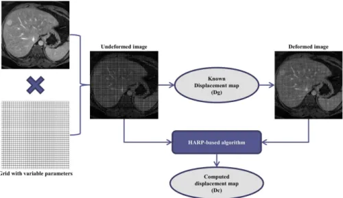
The simulation study was completely performed using a library developed in-house for MATLAB (MATLAB R2013a, Math-Works, Natick, MA). The program generated several sets of tagged MRI images of the liver with various acquisition parameters and known deformations, which simulated liver movements during the cardiac contraction.
Data generation
To simulate realistic tagged MRI images with variable acquisition parameters, digital grids were generated as the product of two orthogonal sets of periodic patterns of tags. Two different grid orientations (0 and 45 degrees) were combined with tag spacings varying from 4 to 7 pixels and a tag thickness equal to the nearest integer value of a third of the tag spacing. The simulated two-dimensional images were obtained by multiplying each simulated grid by a noise-free liver MRI image of 3206320 pixels.
To take into account the Partial Volume Effect (PVE), which occurs in real images when the spacing between lines of the grid is not a multiple of the pixel size, we used a step size of 0.1 for tag spacing variation. Corresponding images were accordingly gener-ated by tagging the interpolgener-ated original image (an oversampling factor of 10 was applied in each spatial direction) with a proper grid. The actual 3206320 matrix was then reconstructed using an
integral subsampling of the tagged image.
In this way, we obtained a total of 62 different simulated undeformed images (Figure 1).
Object deformation
To obtain the deformed images, four 2D continuous displacements maps (Figure 2a) of increasing amplitude were created by generating two smooth and well behaved functions for each amplitude using MATLAB’s ‘‘peaks’’ function to describe the horizontal and vertical displacements, respectively (ground truth Dg1x = Dg1y = [20.4, 0.6] pixels; Dg2x = Dg2y = [2
1.2, 1.7] pixels; Dg3x = Dg3y = [22.0, 2.8] pixels; Dg4x =
Dg4y = [22.7, 3.9] pixels). For each displacement map, the
corresponding image was generated by interpolating the original image on the deformed grids.
As in real tagged MRI, tags persisted according to the longitudinal relaxation time of the tissue. The T1 relaxation effect was taken into account, simulating tag fading in the deformed images within frames during the cardiac cycle. This fading was modelled by multiplying the magnetization of the tags by the
factor1{e{t=T1, whereT1= 850 ms is the estimated longitudinal
relaxation time of the liver at 3T [20] andt= 400 ms is the time frame considered to simulate the end-systolic cardiac phase in the worst case of a very low heart rate.
In summary, for each undeformed image, we obtained four images deformed by displacement maps of different amplitude that simulated the end-systolic frame for different values of liver stiffness (Figure 3).
Noise modeling
To include noise in the simulation, the simulated images were corrupted with different levels of Rician noise [21]. In this model, the real and imaginary parts of the complex MRI images are considered to be corrupted by white additive Gaussian noise with the same noise variance that is transformed into Rician noise by taking the magnitude of the complex data:
Ir~Azg1,g1*Nð0,snÞ
Ii~g2,g2*Nð0,snÞ
m~
ffiffiffiffiffiffiffiffiffiffiffiffiffiffiffiffi Ir2zIi2 q
,
ð1Þ
whereAis the noise free image,Iris the real component,Iiis the imaginary component,snis the standard deviation of the added white Gaussian noiseg, andmis the noisy magnitude image. To determine a realistic power of noise for our simulations, we measured the variance of a background region in a real acquired image, where the noise has a Rayleigh distribution. The noise powers2nwas estimated from the measured variances
2
Musing the relation described in [22]:
s2
M~ 2{
p
2
s2
n, ð2Þ
As the value ofsnobtained in real tagged images acquired at 3T was 2.5% of the maximum intensity of the image, for our simulation, we tested realistic SNRs of 1.5, 2.5, and 3.5%. In summary, for each noise level, 31 different tag spacings at two different orientations were considered for the four deformation fields for a total of 248 simulations.
Data analysis
The displacement maps for each simulation were obtained with in-house software that implements a HARP-based algorithm [11,12] improved by a Gabor filter bank [23].
A tagged image can be considered to be composed of two spatial signals: the background anatomy, located at low frequencies in the Fourier domain, and the overlapped grid, whose signal is represented by two sets of orthogonal harmonic spectral peaks (one for each periodical pattern of tags) centered at multiples of the tagging frequency. The idea of the HARP
algorithm is that the spectral energy corresponding to the motion of the tissue is localized around the first harmonic spectral peak of each set.
To extract this motion information, the groups of images (one undeformed and four deformed) with the same grid parameters were input into a Gabor filter bank. The filter bank was centered
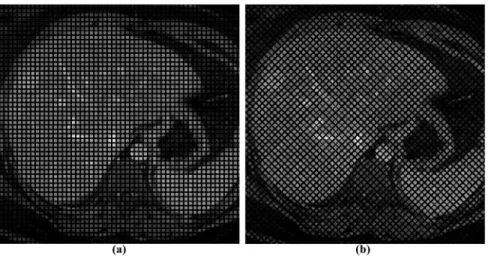
Figure 1. Undeformed images.Images with a tag spacing of 6 pixels and grid angle of (a) 0uand (b) 45u. doi:10.1371/journal.pone.0111852.g001
Figure 2. Ground truth and computed displacement maps.(a) Map of the deformation field Dg2applied in both the x and y directions (Dg2x
= Dg2y = [21.2, 1.7] pixel) of the undeformed image. (b) Estimated displacement map in the x direction (Dcx) and (c) in the y direction (Dcy),
obtained from tagged MRI images with grid angle of 0u, tag spacing of 5 pixels, and deformed by Dg2. (d) Estimated displacement maps in the x
direction (Dcx) and (e) in the y direction (Dcy) obtained from tagged MRI images with a grid angle of 0u, tag spacing of 5 pixels, and deformed by Dg2
at a spatial frequency that corresponded to the first harmonic spectral peak of a periodical pattern of tags. The operation was repeated while changing the central frequency of the bank to extract the peaks corresponding to the other direction of the tags. In summary, for each periodical pattern of tags, we chose a bank composed of nine filters centered around ðuo,voÞ, the frequency of the first harmonic peak in the Fourier domain, which can be expressed in polar coordinates as:
u0~ 1
tagsp
:cosh
v0~ 1
tagsp
:sinh,
ð3Þ
withtagspequal to the tag spacing (measured in pixels) andhequal to the orientation of the set of lines considered. The exact position in the Fourier domain of each filter isðu,vÞ:
u~ 1
m:tagsp
:cosðhzDhÞ
v~ 1
m:tagsp
:sinðhzDhÞ,
ð4Þ
where ðm,DhÞ belongs to the Cartesian product of M~f0:5;1;1:5g and DH~ { p=36;0;zp=36 to cover typical tag rotations and translations.
For both tag directions, the final filter output was calculated by a voxel-based interpolation among the three strongest filter responses at each point in the image, obtaining two complex images, which are the result of an inverse Fourier transform of an asymmetric spectrum and are called harmonic images:
Iiðx,tÞ~Diðx,tÞejwi xð,tÞ, ð5Þ
where Di and wi are the magnitude and phase images, respectively, and i indicates the spectral peak from which the harmonic image is derived (i = 1, 2). Defining the location of the spectral peaks as W~ðv1,v2Þ the information about the 2D
displacement field of the image, u~ðu1,u2Þ, is contained in the
phase image, in fact:
wðx,tÞ~WTx{WTu: ð6Þ
From (6), the displacement field was computed by subtracting the unwrapped phase images obtained from a deformed image and the corresponding undeformed one:
u xð ,tÞ~ WT{1D
wðx,tÞ: ð7Þ
The computed displacement maps are denoted as Dci (Figure 2).
The overall process of data generation and processing is schematically represented in Figure 4.
Statistical evaluation
To evaluate the estimation accuracy for each set of grid parameters (grid orientations = 0uand 45u, tag spacings = 4,7 pixels), applied displacement (Dgix and Dgiy, i = 1, 2, 3, 4), and
three noise levels (1.5, 2.5, and 3.5%), an Error Index (EI) was calculated as:
EI~1 2:
s½Dcx{Dgx
s½Dgx
zsDcy
{Dgy
s Dgy
!
, ð8Þ
whereDcx,Dgx,Dcy, andDgy, respectively represent the estimated and applied displacement maps in the x and y directions, ands
represents the standard deviation operator over the voxel sample. We calculated EI for all simulations to evaluate how the amplitude of the applied deformation, tag spacing, grid angle, and noise level influence the estimation accuracy.
A pair-sample one tailed t-test was used to determine the statistical significance of differences in the EI trends. Statistical analysis was performed using R (R Foundation for Statistical Computing, Vienna, Austria (http://www.R-project.org). A threshold of p,0.05 was considered to be statistically significant.
Figure 3. Deformed images.Images with tag spacing of 6 pixels and grid angle of (a) 0uand (b) 45u, deformed according to Dg4. Fading of the
grid is also applied.
doi:10.1371/journal.pone.0111852.g003
Results
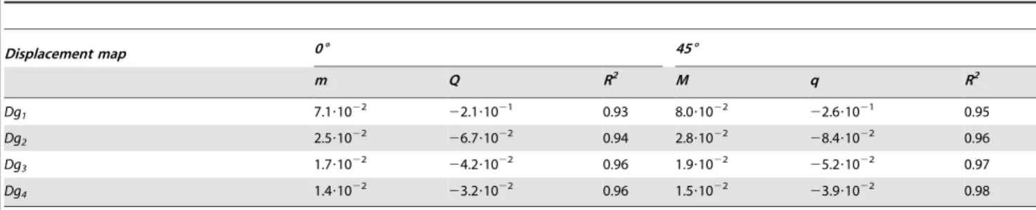
EI values were plotted for each ground truth and both grid angles as a function of tag spacing for the noise-free images (Figure 5). Data were fitted with a linear function, as shown in Table 1, where slope (mDgi, angle) and intercept (qDgi, angle) values
for each Dgias well as both 0uand 45ugrid angles were reported.
In the absence of noise and for each ground truth, the estimation accuracy of the displacement field increased as the tag spacing decreased (all regression slopes were positive) over the observed tag spacing interval.
For all tag spacings and both grid orientations, the EIs were smaller when the amplitude of the ground truth was higher. Furthermore, the differences in EI values obtained for the various tag spacings decreased for increasing Dg. In particular, for the two grid orientations, both the absolute value of the intercept and the slope of the regressions decreased with increasing Dg For displacements on the order of pixel size or less (Dg1), the EIs dropped from a value of 30% for a tag
spacing of 7 pixels to less than 10% for a tag spacing of 4 pixels. For greater displacements, in the order of 3–4 pixels,
Figure 4. Simulation algorithm.Schematic representation of data generation and data processing steps. doi:10.1371/journal.pone.0111852.g004
Figure 5. EI in a noise-free simulation.Plot of EI for each Dgiand for grid angles of 0uand 45uas a function of tag spacing.
accuracy was also high, with higher values of tag spacing (the EI ranged between 3 and 7%).
For each ground truth, the estimation of the displacement map obtained at 0u was more accurate than the estimation at 45u, as expected because of PVE. The difference was statistically significant for Dg1–3–4 and approached significance for Dg2
(pair-sample one tailed t-test: p = 0.03 for Dg1, p = 0.07 for Dg2,
p = 0.03 for Dg3, and p = 0.003 for Dg4). Moreover, for a 0ugrid
orientation, local minima were found to correspond to multiples of pixel size, i.e., in the absence of PVE.
Given these observations, further analyses were conducted only for a grid orientation of 0u.
When noise was added, the smoothness of the displacement measurement was affected (Figures 2(d)–(e)). Plots of EIs calculated for each Dgi and the three levels of noise as a function of tag
spacing are shown in Figure 6. Fitting the new calculated EIs with linear functions (Table 2), it can be observed that the slope of the linear fit decreased for each increase in the level of noise, negating almost completely the advantage of using the smallest tag spacing.
This was particularly true for Dg1at the maximum level of noise
(the EI remained over 25%, even at tag spacing of 4).
The optimal tag spacing turned out to be the smallest multiple of the pixel size (4 pixels) for almost all situations considered. The very few exceptions referred to the smallest deformation in the presence of the highest level of noise, where a value of 5 was preferable.
Discussion
We simulated several acquisition setups and demonstrated how varying tag spacing and grid angle influences the accuracy of motion estimates. We also showed how realistic levels of noise affected the results. The PVE was also taken into account for tag spacings that were not multiples of the pixel size as well as the T1 relaxation that causes grid fading.
The amplitude of the simulated displacements, for typical pixel sizes of real abdominal acquisitions, fell within the range of the observed liver movements in normal and cirrhotic patients (1,5 mm) [8,14,15].
Table 1.Error index in noise-free simulation fitted to linear equation y = mx+q.
Displacement map 06 456
m Q R2 M q R2
Dg1 7.1?1022 22.1?1021 0.93 8.0?1022 22.6?1021 0.95
Dg2 2.5?1022 26.7?1022 0.94 2.8?1022 28.4?1022 0.96
Dg3 1.7?1022 24.2?1022 0.96 1.9?1022 25.2?1022 0.97
Dg4 1.4?1022 23.2?1022 0.96 1.5?1022 23.9?1022 0.98
doi:10.1371/journal.pone.0111852.t001
Figure 6. EI in the presence of noise.Plot of EI for tag spacings varying from 4.0 to 7.0 pixels, a grid angle of 0u, and different noise levels for (a) Dg1, (b) Dg2, (c) Dg3, and (d) Dg4.
doi:10.1371/journal.pone.0111852.g006
In the absence of noise, displacement estimation accuracy improved as the grid tag spacing decreased and became optimal for small displacements (pixel size or less). Comparing the values of EI at different orientations, the estimation of the displacement fields for each Dg was more accurate for a grid angle of 0uover the total range of calculated tag spacings.
The simulation of different levels of noise, similar to those measured on real acquisitions performed at 3T, showed that the smaller tag spacings, identified as optimal in the noise-free simulation, were more sensitive to the presence of noise. This is a crucial point because it is difficult to design an ad-hoc image denoising step. In fact, there is no simple linear relationship between the noise statistics in the displacement estimates and the noise statistics in the image, which undergoes a nonlinear transformation when the phase is computed.
The result of noise addition thus reduces or even cancels out the improvement in accuracy at small values of tag spacing, especially for the smallest ground truth. This imposes a lower theoretical limit on the width of the tag spacing that guarantees appropriate noise rejection. The optimal tag spacing was 4 pixels for almost all the situations considered except Dg1. However, the
results showed EIs comparable to those obtained at a tag spacing of 5 pixels for increasing levels of noise. The lower tag spacing limit had to be combined with the physical limit of the tag spacing boundary values obtainable in a real acquisition that depends on the implementation of the tagging sequence RF pulses on the specific MR scanner used. Another parameter that is dependent on the sequence pulse implementation is tag thickness. In our simulation, we used a fixed value equal to the nearest integer to one third of the tag spacing. However, this should not be a crucial point in our analysis because the HARP method should not be substantially sensitive to variation in this parameter, unlike line tracking methods that require an accurate estimation of the tag centerline position [18].
We limited our simulation to values of T1 relaxation time that are typical for liver at 3T, but this is not an obstacle to a broader application of our results. The shorter T1 at lower magnetic field intensities [20] causes a faster tag fading and affects the CNR of the tags [24]. Hence, if we simulated an acquisition in this condition, we would expect estimation results comparable to the ones obtained with the same T1 and a higher power of noise. Analogously, the heart rate may influence the CNR of the tags, according to the Bloch equation for the T1 recovery of the tagged tissues. This is because the end-systolic cardiac phase may occur at different delays, thus affecting grid fading.
In conclusion, we suggest the use of a grid angle of 0uand, for all noise levels, a value of tag spacing that is a multiple of the pixel spacing to avoid PVE and for which the EI reached local minimums. This is because in the presence of PVE, if a pixel in a harmonic image is the mean of several complex numbers, expressed as (5), there will be an error in the displacement measurement. This occurs because the resulting phase of the pixel is not equal to the average of all the component phases, as it is a nonlinear function. Hence, the optimal tag spacing should be a compromise between the smallest tag period (a multiple of the pixel spacing) achievable in a real acquisition and the tag spacing that guarantees appropriate noise rejection in the presence of a realistic level of noise (given the scanner used for acquisition).
We believe that future work is needed to verify the impact of the optimization of the tagging MR acquisition parameters in clinical studies as well as to accurately quantify the extent of liver displacement expected at the various fibrosis stages.
Author Contributions
Conceived and designed the experiments: SM GP AP. Analyzed the data: SM GP AP MR. Contributed reagents/materials/analysis tools: SM GP
AP LM. Wrote the paper: SM GP AP MM LM. Developed the software used in analysis: SM GP.
References
1. Muthupillai R, Ehman RL (1996) Magnetic resonance elastography. Nat Med 2: 601–603.
2. Mariappan YK, Glaser KJ, Ehman RL (2010) Magnetic resonance elastography: a review. Clin Anat 23: 497–511.
3. Huwart L, Sempoux C, Vicaut E, Salameh N, Annet L, et al. (2008) Magnetic resonance elastography for the noninvasive staging of liver fibrosis. Gastroen-terology 135: 32–40.
4. Rouviere O, Yin M, Dresner MA, Rossman PJ, Burgart LJ, et al. (2006) MR elastography of the liver: preliminary results. Radiology 240: 440–448. 5. Rustogi R, Horowitz J, Harmath C, Wang Y, Chalian H, et al. (2012) Accuracy
of MR elastography and anatomic MR imaging features in the diagnosis of severe hepatic fibrosis and cirrhosis. J Magn Reson Imaging 35: 1356–1364. 6. Yin M, Talwalkar JA, Glaser KJ, Manduca A, Grimm RC, et al. (2007)
Assessment of hepatic fibrosis with magnetic resonance elastography. Clin Gastroenterol Hepatol 5: 1207–1213 e1202.
7. Kim BH, Lee JM, Lee YJ, Lee KB, Suh KS, et al. (2011) MR elastography for noninvasive assessment of hepatic fibrosis: experience from a tertiary center in Asia. J Magn Reson Imaging 34: 1110–1116.
8. Chung S, Breton E, Mannelli L, Axel L (2011) Liver stiffness assessment by tagged MRI of cardiac-induced liver motion. Magn Reson Med 65: 949–955. 9. Zerhouni EA, Parish DM, Rogers WJ, Yang A, Shapiro EP (1988) Human
heart: tagging with MR imaging – a method for noninvasive assessment of myocardial motion. Radiology 169: 59–63.
10. Axel L, Dougherty L (1989) MR imaging of motion with spatial modulation of magnetization. Radiology 171: 841–845.
11. Osman NF, McVeigh ER, Prince JL (2000) Imaging heart motion using harmonic phase MRI. Medical Imaging, IEEE Transactions on 19: 186–202. 12. Osman NF, Kerwin WS, McVeigh ER, Prince JL (1999) Cardiac motion
tracking using CINE harmonic phase (HARP) magnetic resonance imaging. Magn Reson Med 42: 1048–1060.
13. Kumar S, Goldgof D (1994) Automatic tracking of SPAMM grid and the estimation of deformation parameters from cardiac MR images. IEEE Trans Med Imaging 13: 122–132.
14. Mannelli L, Wilson GJ, Dubinsky TJ, Potter CA, Bhargava P, et al. (2012) Assessment of the liver strain among cirrhotic and normal livers using tagged MRI. Journal of Magnetic Resonance Imaging 36: 1490–1495.
15. Chung S, Kim KE, Park MS, Bhagavatula S, Babb J, et al. (2014) Liver stiffness assessment with tagged MRI of cardiac-induced liver motion in cirrhosis patients. J Magn Reson Imaging 39: 1301–1307.
16. Crum WR, Berry E, Ridgway JP, Sivananthan UM, Tan LB, et al. (1997) Simulation of two-dimensional tagged MRI. J Magn Reson Imaging 7: 416– 424.
17. Crum WR, Berry E, Ridgway JP, Sivananthan UM, Tan LB, et al. (1998) Frequency-domain simulation of MR tagging. J Magn Reson Imaging 8: 1040– 1050.
18. Atalar E, McVeigh ER (1994) Optimization of tag thickness for measuring position with magnetic resonance imaging. IEEE Trans Med Imaging 13: 152– 160.
19. Reeder SB, McVeigh ER (1994) Tag contrast in breath-hold CINE cardiac MRI. Magn Reson Med 31: 521–525.
20. de Bazelaire CMJ, Duhamel GD, Rofsky NM, Alsop DC (2004) MR Imaging Relaxation Times of Abdominal and Pelvic Tissues Measured in Vivo at 3.0 T: Preliminary Results. Radiology 230: 652–659.
21. Henkelman RM (1985) Measurement of signal intensities in the presence of noise in MR images. Med Phys 12: 232–233.
22. Papoulis A (1991) Probability, Random Variables, and Stochastic Process. 3.: McGraw-Hill INC.
23. Montillo A, Metaxas D, Axel L (2004) Extracting tissue deformation using Gabor filter banks. In Proc of SPIE: Medical Imaging: Physiology, Function, and Structure from Medical Images 5369: 1–9.
24. Ryf S, Koaerke S, Spiegel M, Lamerichs R, Boesiger P (2002) Myocardial Tagging: Comparing Imaging at 3.0 T and 1.5 T. In Proc of Intl Soc Mag Reson Med 10.