Cost Minimization Model of Gas Transmission Line
for Indonesian SIJ Pipeline Network
Septoratno Siregar1, 3, Edy Soewono2, 3, Daniel Siregar3, Satya A. Putra 4 & Yana Budicakrayana4 1
Department of Petroleum Engineering, Institut Teknologi Bandung 2
Department of Mathematics, Institut Teknologi Bandung 3
Research Group for Industrial & Applied Mathematics, Institut Teknologi Bandung 4
PERTAMINA
Abstract. Optimization of Indonesian SIJ gas pipeline network is being discussed here. Optimum pipe diameters together with the corresponding pressure distribution are obtained from minimization of total cost function consisting of investment and operating costs and subjects to some physical (Panhandle A and Panhandle B equations) constraints. Iteration technique based on Generalized Steepest-Descent and fourth order Runge-Kutta method are used here. The resulting diameters from this continuous optimization are then rounded to the closest available discrete sizes. We have also calculated toll fee along each segment and safety factor of the network by determining the pipe wall thickness, using ANSI B31.8 standard. Sensitivity analysis of toll fee for variation of flow rates is shown here. The result will gives the diameter and compressor size and compressor location that feasible to use for the SIJ pipeline project. The Result also indicates that the east route cost relatively less expensive than the west cost.
1 Introduction
With large natural gas resources and the increase demand of domestic gas consumption in Indonesia, the need to extend the existing pipeline network and to build new pipelines connecting several resources and consumers has been growing significantly in the last decade. In order to connect the gas fields to the costumers which are normally several hundred kilometers away, it is very important to build an integrated and efficient transmission pipeline. The role of optimization techniques is very crucial to minimize the investment and operating cost.
Several commercial softwares being used in gas industries are not directly built on the basis of cost optimization. Here we use mathematical model for the pipeline cost as a function of pipe diameters and pressures, which satisfy some physical constraints. Relevant technical, economical and physical aspects related to investment and operating costs are taken into account. There are several literatures on pipe line optimization (see for example in [1, 2, 3]), most of them use simplified model either in the construction of cost function or in the constraints. Recently a complete cost model which is suitable for Indonesian gas fields was proposed in [4]. This model turns to be useful both for transporter companies and gas field owners. Applications of the model in different fields and different conditions could be seen in [5, 6]. This cost model is presented in section 4. This cost function will be the objective function for our optimization. In section 3, we review Panhandle A and Panhandle B equations describing the flow equation in each segment of pipes. This flow equation together with maximum pressure in each segment and maximum discharge pressure of compressors will function as constraints for the minimization techniques which are described in section 6. Wall thickness calculation which is related to the strength of the pipe is discussed in section 5.
The optimum diameters that are obtained from the optimization process will be adjusted to the nearest sizes which are available in the market. The safety factor of the pipeline will be calculated by determining the pipe wall thickness using ANSI B.31 standard. These results are also adjusted to the real sizes available in the market.
2
Description of SIJ Network
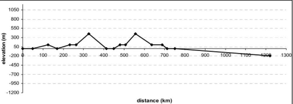
SIJ pipeline transmission network is to be chosen between two possible (west and east) routes, both connecting the inlet point A with the outlet point SN as shown in figure 1. The total length of each route is about 1200 km. Only the segment OF-SN lie off-shore and the rest of the network lies on-shore. In order to anticipate large pressure drop, compressor are planned to be located in four positions.
Figure 2 Elevation map (west route). -1200
-950 -700 -450 -200 50 300 550 800 1050
0 100 200 300 400 500 600 700 800 900 1000 1100 1200 1300
distance (km )
e
lev
at
io
n
(
m
)
East Route West Route
-1200 -950 -700 -450 -200 50 300 550 800 1050
0 100 200 300 400 500 600 700 800 900 1000 1100 1200 1300
distance (km)
el
e
vat
io
n
(
m
)
Figure 3 Elevation map (east route).
3 Pipe Flow Equation
Flow equation in a single segment of transmission pipeline is generally derived from the steady state condition of the energy balance equation, taking into account the empirical friction factor .The equation is written in term of pressure gradient as follows [7]
dl g
vdv d
g v f g
g dl dp
c c c
ρ ρ θ
ρ + +
=
2 sin
2
, (1) where
f = friction factor
θ
= angle of elevationThrough out this paper we consider the case of steady state flow; therefore equation (1) is reduced to steady state flow equation
d g
v f g
g dl dp
c
c 2
sin
2
ρ θ
ρ +
= . (2)
Here we assume that the adiabatic condition prevails and temperature through out the pipe is constant. Friction between gas and inside wall of the pipe will cause a loss of mechanical energy during the flow. This energy loss depends on the viscosity of the gas and the roughness of inside wall. The friction factor depends also on the flow rate of the gas and the pipe diameter. Two models of friction factor are used here, which are Panhandle A and Panhandle B, as shown in equation (3) and (4),
147 . 0 Re 085 . 0 N
0392 . 0 Re 015 . 0
N
f = (4)
respectively. Note that the flow equation (2) will function as a constraint relating pressure and diameter in each segment of pipe.
4
Cost Model Structure
In this section the construction of the total cost model adopted from [4] will be discussed. This total cost will be used as the objective function for the optimization process. The cost is separated into two parts, the (total) pipe cost and the (total) compressor cost as follows
with some assumptions ,
a) gas in the pipeline is single-phase flow
b) gas flow in the pipeline is steady state
c) gas temperature along each segment of pipe is constant
d) gas temperature does not change after coming out of compressor
e) gas deviation factor (Z) along each segment of pipe is constant and does not change after coming out of compressor
f) compressor type is centrifugal
g) tax, insurance, and other economic calculations are excluded.
Investment Cost
Here a uniform capital recovery is used for annual investment cost. The formula is given as follows
1 ) 1 (
) 1 (
− +
+
= nn
r r r P
A (5) TOTAL
COST
INVESTMENT COST
=
+
+
OPERATION COSTINVESTMENT
COST
+
OPERATION COST
PIPE
where
A = uniform annual capital cost
P = present value of total investment cost
r = annual interest rate
n = life time of the equipment.
Investment Cost for Pipeline
The total investment cost for a segment of pipe is given as follows
m l
d CpL Rp
Cpipe=(1+ ) (6) where
Cpipe = pipe investment cost (US$)
Rp = ratio between pipe installation cost and the pipe price itself
Cp = unit price of pipe (US$/ft.inch), obtained from available data
L = length of pipe (feet)
d = diameter of pipe (inch)
l,m = non-linearity constants obtained from regression.
The total investment cost for piping consists of pipe material, and installation cost. The annual cost based on capital recovery approach as indicated in equation (5) is
1
) 1 (
) 1 ( ) 1 (
− +
+ +
= n n l m
r
d CpL Rp r
r CIP
(7) where
CIP = annual investment cost of pipe (US$/year)
r = annual interest rate.
Compressor Investment Cost
Investment cost of compressor is given by the following model
Ccomp = Chp ghp b
where
Chp = compressor price (US$/hp)
ghp = compressor power (hp)
The compressor is centrifugal type. Based on the above assumptions, the power of compressor can be written as
sl bl k Tb k P P Z T Pb Q ghp Ep k k + + − − = − ) 1 ( 1 2061 6250 1 1 2 (8) where
Q = inlet gas flow-rate for the compressor (MMscfd)
Pb = base pressure (psia)
Tb = base temperature (oR)
T = gas temperature (oR)
Z = gas deviation factor
P1 = inlet pressure (psia)
P2 = outlet pressure (psia)
k = adiabatic exponent
Ep = efficiency of compressor (%)
bl, sl = bearing losses and seal losses.
The total investment cost for compressor is obtained as follows
b Ep k k sl bl k Tb k P P Z T Pb Q Chp Ccomp + + − − = − ) 1 ( 1 2061 6250 1 1 2 (9)
b Ep k k n n sl bl k Tb k P P Z T Pb Q Chp r r r CIC + + − − − + + = − ) 1 ( 1 2061 6250 1 ) 1 ( ) 1 ( 1 1 2 (10)
Pipeline Operating Cost
The annual operating cost of pipeline is assumed to be proportional to the pipe investment cost as follows
1 ) 1 ( ) 1 ( ) 1 ( − + + +
= n n l m
r d L Cp Cfp Rp r r
OCpipe (11)
where
Ocpipe = pipe operating cost (US$/year)
Cfp =fraction, a ratio of pipe operation cost to investment cost.
Compressor Operating Cost
Factors affecting the compressor operating cost are electricity cost for compressor operation (if electricity is used), maintenance cost, and other costs involved in compressor system.
The operating cost is proportional to the electricity cost, as follows
OCcomp = xLstr
with
x
>
1
and Lstr represents the electricity cost. For convenience, x is written asx = 1 + Copcomp
with Copcomp represents a fraction of compressor operating cost excluding its electricity cost. The compressor operating cost can be written as
OCcomp = (1 + Copcomp) Lstr.
To obtain the electricity cost, the unit used in equation (8) is converted from
(
)
.(
bl sl)
CeHy k Tb k P P Pb T Z Q . Lstr kEp k + + − − = − 321518 6532 1 1 32047 19809 8760 1 1 1 2 (12) whereCe : electricity cost (US$/Kwh)
Hy : operating compressor hours in a year.
Toll Fee
Toll fee is a service fee for delivering a unit of gas through a segment of pipeline. Toll fee can be charged per unit length (US$/MSCF/km) or for a certain distance ($/MSCF). Due to the effect of “economic of scale”, toll fee is usually charged on distance basis. An illustration for calculating the toll fee is presented as follows.
a) Consider N segment transmission pipeline, then we have
CIP = CIP1 + CIP2 + … + CIPN (13)
OCpipe = OCpipe1 + OCpipe2 + … + OcpipeN. (14)
b) Gas that flows along the pipeline which is located after compressor is influenced by the compressor power, no matter how small it is. Due to this fact, we will add the CIC and OCcomp costs to each segment of pipe that is influenced by the compressor based on the length of the pipe. Thus, we have
CIC Lf
L
CIC i
i = , (15)
OCcomp Lf
L
OCcomp i
i = (16)
with Li as the length of a segment of pipe which is located after
compressor, and Lf as the total length of all pipes which are located after compressor.
1000 365× ×
+ + +
=
i
i i
i i
i
Q
OCcomp CIC
OCpipe CIP
TF (17)
with
TFi = toll fee on segment of –I (US$/MSCF).
Note that in practice the location of compressors represented by the parameters
Li could be taken as optimizing parameters.
5
Wall Thickness Calculation for Transmission Pipe
Wall thickness calculation of the pipeline is obtained by using ANSI B 31.8 standard [10]. This standard is considering some factors, such as pipe design, diameter, pressure and the type of the pipe. The Equation of the wall thickness is given as
) . . . .( 2
. 0
S T E F
d P
t= (18)
with :
t = wall thickness (inch)
P = pressure (psia)
d0= outside diameter (inch)
S = minimum pipe strength (psi)
F = design factor
E = join factor
T = temperature derating factor.
Design factor depends on the location of the pipe. Some type of design factor can be seen below.
Class Design Type Design Factor
1 2 3 4
Oil and gas field or unpopulated area Semi-developed area, minimum facility
Compressor station area.
Commercials area .
0.72 0.6 0.5 0.4
1.00 for seamless, ERW pipe,
0.80 for furnace lap and electrical fusion welded pipe,
0.60 for furnace butt welded pipe.
Temperature derating factor is a measurement of temperature’s effect to the pipe material. This value gives the relation between the temperature and its impact to the pipe material. The value of this coefficient is given in the table below.
Temperature ( oF) Derating Factor
-20o – 250o 300o 350o 400o 450o
1.000 0.967 0.933 0.900 0.867
6 Optimization
Method
Here we minimize an objective (Total Cost) function, which is nonlinear subject to a set of constraints consisting nonlinear equations and inequalities. We denote the objective function by C(X) and the constraints
2 1 1, ( ) 0, .. ..
1 , 0 )
(X j J K X j J J
Kj = = j ≤ = , where the components of
X
arepipe diameters, gas pressures and compressor horse power, the equality constraints are the flow equations in each segment of pipes, and the inequality constraints are the maximum pressure conditions of pipes which represent the strength of the pipes. Note that the linear technique approach (see for example in [1, 2]) is no longer workable in this model since high non-linearity terms involve in objective function as well as in constraints. Other approach using heuristic techniques were also done (see in [8, 9]). The continuous approach being used here is chosen to accommodate more complicated physical condition such as surface elevation and if necessary the change of temperature can also be included.
From a given initial conditionX0, we select the direction, which gives the largest decrease of the cost. This direction is based on the Generalized
Steepest-Descent which is given by the gradient of each constraint (
∑
=
∇
1
1
) ( J
j
n j
j K X
α
)
.The procedure for constrained minimization is given as follows
] ) ( )
(
1
1
∑
=
∇ +
−∇
= J
j
j
j K X
X C dt
dX α
where t is iteration parameter and
α
jhas to satisfy the system of linearequations
1 1
.. 1 ), ( ) ( ) ( ) (
1
J i X K X C X K X
K i i
J
j
j
j∇ ∇ =∇ ∇ =
∑
=
o o
α . (20)
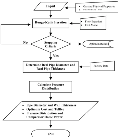
The Fourth Order Runge Kutta method is then applied to the dynamical equation (19) to produce the optimum result. Below is the algorithm for the computational process.
Figure 4 Numerical computation flow chart.
Input • Gas and Physical Properties
• Economics Data
Runge-Kutta Iteration
Optimum Result
Determine Real Pipe Diameter and Real Pipe Thickness
Stopping Criteria No
Yes
Calculate Pressure Distribution
• Pipe Diameter and Wall Thickness
• Optimum Cost and Tollfee
• Pressure Distribution and Compressor Horse Power
Factory Data
END
• Flow Equation
7
Numerical Results and Analysis
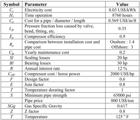
Here we present numerical result for the SIJ pipeline transmission network. The set of data that is used in the computation is given in table 1.
Symbol Parameter Value
Ce Electricity cost 0.03 US$/kWh
Hy Time operation 8760 hours
Cp Cost for a pipe / diameter / length 0.569 US$/in/ft
Lfp
Pressure fraction loss caused by valve,
bend, fitting, etc. 0.35
Ep Compressor efficiency 0.9
Rp
Comparison between installation cost and pipe cost
Onshore : 1.4 Offshore: 3
Cfp Yearly maintenance cost 0.2
Sl Sealing losses 20 hp
Bl Bearing losses 30 hp
R Annual interest rate 12 %
CHP Compressor cost / horse power 2000 US$/hp
F Design factor 0.6
E Join factor 0.8
T Temperature derating factor 1
S Minimum pipe strength 65000 psi
Pipe price 800 US$/ton
SGg Gas Specific Gravity 0.617
Z Z factor 0.8
T Temperature 125 o F
Table 1 Data for Computation.
No Segments Length
(km)
Flowrate
(MMSCF/D)
Elevation
(meter)
1 A-B 50 341 0
2 B-C 75 341 100
3 C-D 43.75 341 0
4 D-E 62.5 841 100
5 E-F 31.25 841 100
6 F-G 62.5 841 400
7 G-H 87.5 841 0
8 H-I1 125 841 400
9 I1-J1 75 841 0
10 J1-K1 50 841 0
11 K1-L1 18.75 841 0
12 L1-M1 25 841 0
13 M1-OF 75 841 0
14 OF-SN 470 841 (200)
No Segments Length
(km)
Flowrate
(MMSCF/D)
Elevation
(meter)
1 A-B 50 341 0
2 B-C 75 341 100
3 C-D 43.75 341 0
4 D-E 62.5 841 100
5 E-F 31.25 841 100
6 F-G 62.5 841 400
7 G-H 87.5 841 0
8 H-I2 37.5 841 0
9 I2-J2 31.25 841 100
10 J2-K2 25 841 100
11 K2-L2 50 841 400
12 L2-M2 81.25 841 100
13 M2-N2 50 841 100
14 N2-O2 25 841 0
15 O2-OF 37.5 841 0
16 OF-SN 470 841 (200)
Table 3 Summary of physical parameters, east scenario.
Pipe specification is X-65. Maximum discharge pressures are controlled not more than 1000 psia. Here we will compare the optimization result between Panhandle A and Panhandle B. The complete data of the pipeline network can be seen in table 2 and 3.
The results of numerical computation and analysis for East and West route will be presented in two forms, which are the optimum result and the practical result.
7.1
Optimum Result
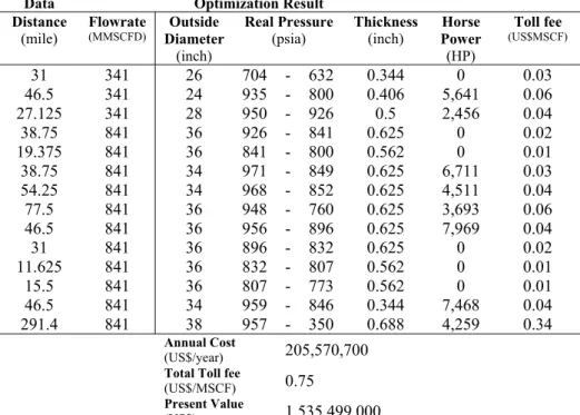
The optimum result is directly obtained from numerical computation, as well as the number and the position of compressors. Here the compressors are placed in every node on the route and the process will eliminate unnecessary compressor in the certain position. At the end, we will obtain the optimum number of compressor in the certain position, beside the optimum diameter and horse power. The result of optimum condition can be seen in table 4 and 5 below.
Data Optimization Result
Distance Flowrate Outside Real Pressure Thickness Horse Toll fee
(mile) (MMSCFD) Diameter (inch)
(psia) (inch) Power
(HP)
(US$MSCF)
31 341 26 704 - 632 0.344 0 0.03
46.5 341 24 935 - 800 0.406 5,641 0.06
27.125 341 28 950 - 926 0.5 2,456 0.04
38.75 841 36 926 - 841 0.625 0 0.02
19.375 841 36 841 - 800 0.562 0 0.01
38.75 841 34 971 - 849 0.625 6,711 0.03
54.25 841 34 968 - 852 0.625 4,511 0.04
77.5 841 36 948 - 760 0.625 3,693 0.06
46.5 841 36 956 - 896 0.625 7,969 0.04
31 841 36 896 - 832 0.625 0 0.02
11.625 841 36 832 - 807 0.562 0 0.01
15.5 841 36 807 - 773 0.562 0 0.01
46.5 841 34 959 - 846 0.344 7,468 0.04
291.4 841 38 957 - 350 0.688 4,259 0.34
Annual Cost
(US$/year) 205,570,700 Total Toll fee
(US$/MSCF) 0.75 Present Value
(US$) 1,535,499,000
Table 4 Optimum result for West Route, using Panhandle A equation.
340 440 540 640 740 840 940
0 100 200 300 400 500 600 700 800 900 1000 1100 1200 1300
Dis tance (km )
P
re
ssu
re (
p
si
a)
Data Optimization Result
Distance Flowrate Outside Real Pressure Thickness Horse Toll fee
(mile) (MMSCFD) Diameter Power (US$/MSCF)
(inch)
(psia) (inch)
(HP)
31.00 341 26 701 - 629 0.344 0 0.03
46.50 341 24 931 - 795 0.406 5,642 0.06
27.13 341 28 944 - 920 0.5 2,456 0.04
38.75 841 36 920 - 835 0.625 0 0.02
19.38 841 36 835 - 793 0.562 0 0.01
38.75 841 34 962 - 840 0.625 6,711 0.03
54.25 841 36 957 - 880 0.625 4,511 0.04
23.25 841 36 880 - 832 0.562 0 0.02
19.38 841 36 832 - 783 0.562 0 0.01
15.50 841 34 972 - 934 0.625 7,512 0.02
31.00 841 34 934 - 830 0.562 0 0.02
50.38 841 36 967 - 892 0.625 5,281 0.04
31.00 841 34 892 - 806 0.562 0 0.02
15.50 841 34 961 - 931 0.625 6,100 0.02
23.25 841 34 931 - 870 0.562 0 0.01
291.40 841 38 957 - 350 0.688 3,291 0.34
Annual Cost
(US$/year) 201,017,000 Total Tollfee
(US$/MSCF) 0.74 Present Value
(US$) 1,501,485,000
Table 5 Optimization result for East Route.
Figure 6 Pressure distribution for Optimum case East Route. 350
450 550 650 750 850 950
0 100 200 300 400 500 600 700 800 900 1000 1100 1200 1300
Distance (k m )
P
res
s
u
re
(
P
si
7.2
Practical Result
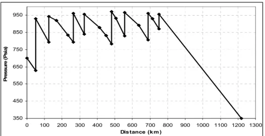
The optimum result may not be practical and applicable in the real condition, because the positions of the compressors are not feasible for practical condition. Here the compressor positions are relocated (if necessary) in selected position or node, with the distance in between 150-200 kilometers each. The result can be seen in table 6 and 7 below.
Data Optimization Result
Distance Flowrate Outside Real Pressure Thickness Horse Toll fee
Diameter Power (US$ /MSCF)
(mile) (MMSCFD)
(inch)
(psia) (inch)
(HP)
31 341 30 736 - 703 0.406 0 0.04
46.5 341 30 703 - 643 0.375 0 0.06
27.125 341 30 643 - 615 0.344 0 0.03
38.75 841 36 974 - 891 0.625 16,309 0.05
19.375 841 36 891 - 852 0.562 0 0.01
38.75 841 36 852 - 747 0.562 0 0.02
54.25 841 36 988 - 916 0.625 9,741 0.05
77.5 841 36 916 - 725 0.625 0 0.05
46.5 841 36 985 - 928 0.625 10,706 0.05
31 841 36 928 - 866 0.625 0 0.02
11.625 841 36 866 - 842 0.562 0 0.01
15.5 841 36 842 - 809 0.562 0 0.01
46.5 841 36 809 - 708 0.344 0 0.03
291.4 841 38 957 - 350 0.688 10,536 0.35
Annual Cost
(US$/year) 212,967,000 Total Toll fee
(US$/MSCF) 0.77 Present Value
(US$) 1,590,745,000
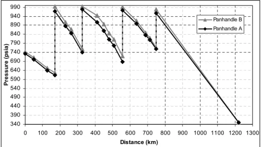
Table 6 Practical-Optimum result for West Route.
340 390 440 490 540 590 640 690 740 790 840 890 940 990
0 100 200 300 400 500 600 700 800 900 1000 1100 1200 1300
Distance (km )
P
ressu
re (
p
si
a)
Panhandle B
Panhandle A
7.3
Analysis
From section 7.1, we obtain the optimum result of SIJ pipeline network. The compressor is located in every node and the numerical process eliminates unnecessary compressor to obtain the optimum number of compressor. For the west route, from 14 compressor placed, the process decrease it into 8 compressor (table 4) and for east route, the number decreases from 16 into 8 compressor (table 5). However, in this case, the numbers of compressor still not suitable for practical utilization, because the distance of each compressor is not long enough. The diameter size is also obtained with various numbers, which make it not practical for real condition, such as if there is any maintaining process, cleaning process, etc.
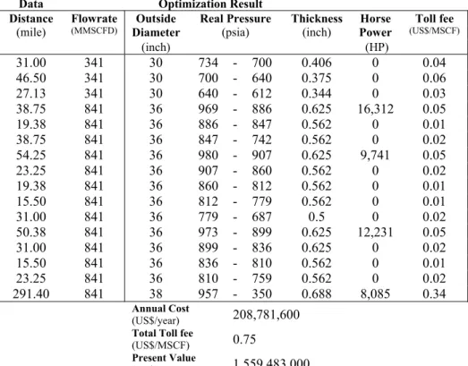
Data Optimization Result
Distance Flowrate Outside Real Pressure Thickness Horse Toll fee
Diameter Power (US$/MSCF)
(mile) (MMSCFD)
(inch)
(psia) (inch)
(HP)
31.00 341 30 734 - 700 0.406 0 0.04
46.50 341 30 700 - 640 0.375 0 0.06
27.13 341 30 640 - 612 0.344 0 0.03
38.75 841 36 969 - 886 0.625 16,312 0.05
19.38 841 36 886 - 847 0.562 0 0.01
38.75 841 36 847 - 742 0.562 0 0.02
54.25 841 36 980 - 907 0.625 9,741 0.05
23.25 841 36 907 - 860 0.562 0 0.02
19.38 841 36 860 - 812 0.562 0 0.01
15.50 841 36 812 - 779 0.562 0 0.01
31.00 841 36 779 - 687 0.5 0 0.02
50.38 841 36 973 - 899 0.625 12,231 0.05
31.00 841 36 899 - 836 0.625 0 0.02
15.50 841 36 836 - 810 0.562 0 0.01
23.25 841 36 810 - 759 0.562 0 0.02
291.40 841 38 957 - 350 0.688 8,085 0.34
Annual Cost
(US$/year) 208,781,600 Total Toll fee
(US$/MSCF) 0.75 Present Value
(US$) 1,559,483,000
Table 7 Optimization-practical result for East Route.
The offshore pipeline is about 470 km, and only uses 1 compressor with discharge pressure at 1000 psia. This condition happens because it is not preferable to put a compressor station in the middle of the ocean. Due this condition, the pipe diameter on the offshore area has to be larger than the onshore pipeline diameter, which is 38 inches.
8 Sensitivity
Analysis
A sensitivity analysis is usually performed to observe the changes of variable of interest due to the changes of parameter. Here we make some sensitivity analysis for toll fee, with respect to flow rate. The result can be seen in figure 7.
0.65 0.7 0.75 0.8 0.85 0.9 0.95
400 500 600 700 800 900 1000 1100 1200
Flow rate (MMSCFD)
Tol
lf
e
e
($
/M
S
C
F
)
West Route
East Route
Figure 9 Toll fee sensitivity analysis.
340 390 440 490 540 590 640 690 740 790 840 890 940 990
0 100 200 300 400 500 600 700 800 900 1000 1100 1200 1300
Distance (km)
P
ressu
re (
p
si
a)
Panhandle B Panhandle A
The optimization result is also giving a different result of diameter. The larger flow rate implies the larger diameter, but gives smaller toll fee value.
9 Conclusion
We have presented the optimum SIJ transmission (east and west) networks resulting from minimization of total cost function subject to constraints in the forms of flow equation in each segment pipe, maximum strength of pipe and additional constraints related to compressor. The computations are performed with fourth order Runge Kutta method. The optimum diameters resulting from the continuous optimization are then being used to find the closest sizes available in the market. Results indicate that the east route is relatively less expensive than the west route.
Acknowledgment
The authors would like to thank the Research Consortium OPPINET for funding the research.
References
1. De Wolf, D., Smeers, Y., Optimal Dimensioning of Pipe Networks with
Application to Gas Transmission Network, Operation Research v. 44, 1996, 596-608.
2. De Wolf, D., Smeers, Y., The Gas Transmission Problem Solved by an
Extension of the Simplex Algoritm, to appear in Management Science.
3. Osiadacz, A.J., Gorecki, M., Optimization of Pipe sizes for Distribution
Gas Network Design, PSIG 9511, 1995.
4. Arsegianto, Soewono, E., Apri, M., Non-Linear Optimization Model for
Gas Transmission System: A Case of Grissik - Duri Pipeline, to appear in SPE 80506.
5. Siregar, S., Soewono, E., Mucharam, L., Sidarto, K.A., Arsegianto,
Chaerani, D., Mubassiran, Research on Gas Pipeline Network Modelling
In Order to Anticipate Development of National Gas Pipeline Network (Indonesian), Proc. Lokakarya Gas II, PERTAMINA, 2001, 219-224.
6. Siregar, S., Soewono, E., Mucharam, L., Putra, Satya A., Udayana, W.T.,
Wangsadiputra, A., Siregar, D., Optimization of Gas Pipeline Network in
7. Ikoku, Chi U., Natural Gas Production Engineering, J. Wiley, 1984.
8. Xue, G., Lillys, T.P., Dougherty, D.E., Computing the Minimum Cost
Pipe Networks Interconnecting One Sink and Many Sources, SIAM J. OPTIM Vol. 10, No. 1, pp 22 42, 1999.
9. Soewono, E, Siregar, S., Widiasri, I. S., Ariani, N., Optimization for
Large Gas Transmission Network Using Least Difference Heuristic Algorithm, will be presented in International Conference 2003 on Mathematics and its Application, Yogyakarta, 14-17 July 2003.
10. Arnold, K., Steward, M., Surface Production Operation vol. 1, Gulf