doi: 10.1590/0101-7438.2014.034.03.0395
COMPLEXITY OF FIRST-ORDER METHODS FOR DIFFERENTIABLE CONVEX OPTIMIZATION
Cl´ovis C. Gonzaga
1and Elizabeth W. Karas
2*Received December 8, 2013 / Accepted February 9, 2014
ABSTRACT.This is a short tutorial on complexity studies for differentiable convex optimization. A com-plexity study is made for a class of problems, an “oracle” that obtains information about the problem at a given point, and a stopping rule for algorithms. These three items compose ascheme, for which we study the performance of algorithms and problem complexity. Our problem classes will be quadratic minimiza-tion and convex minimizaminimiza-tion inRn. The oracle will always be first order. We study the performance of steepest descent and Krylov space methods for quadratic function minimization and Nesterov’s approach to the minimization of differentiable convex functions.
Keywords: first-order methods, complexity analysis, differentiable convex optimization.
1 INTRODUCTION
Due to the huge increase in the size of problems tractable with modern computers, the study of problem complexity and algorithm performance became essential. This was recognized very early by computer scientists and mathematicians working on combinatorial problems, and has recently become a central issue in continuous optimization. Complexity studies for these prob-lems started in the former Soviet Union, and the main results are described in the book by Nemirovski & Yudin [14].
The special case of Linear Programming, which will not be tackled in this paper, initiated with Khachiyan [10], also in Russia in 1978, and had an explosive expansion in the West with the creation of interior point methods in the 80’s and 90’s.
This paper starts with a brief introduction to the main concepts in the study of algorithm per-formance and complexity, following Nemirovski and Yudin, and then apply to the study of the convex optimization problem:
minimize
x∈Rn f(x), (1)
*Corresponding author.
1Department of Mathematics, Federal University of Santa Catarina, Cx. Postal 5210, 88040-970 Florian´opolis, SC, Brazil. E-mail: [email protected]
where f :Rn →Ris a continuously differentiable function.
In Section 2 we introduce the general framework for the study of algorithm performance and problem complexity and present a simple example.
We dedicate Section 3 to study the special case of convex quadratic functions, because they are the simplest non-linear functions: if a method is inefficient for quadratic problems, it will certainly be inefficient for more general problems; if it is efficient, it has a good chance of being adaptable to general differentiable convex problems, because near an optimal solution the quadratic approximation of the function uses to be precise. We study the performance of steepest descent and of Krylov space methods.
Section 4 will describe and analyze a basic method for unconstrained convex optimization de-vised by Nesterov [15], with “accelerated steepest descent” iterations. This method has become very popular, and the presentation and complexity proofs will be based on our paper [7].
Finally, we comment in Section 5 on improvements of this basic algorithm, presenting without proofs its extension to problems restricted to “simple sets” (sets onto which projecting a vector is easy).
2 SCHEMES, PERFORMANCE AND COMPLEXITY
A complexity study is associated with a scheme(,O, τε)as follows.
(i) is a class of problems.
Examples: linear programming problems, unconstrained minimization of convex func-tions.
(ii) Ois an oracle associated to.
The oracle is responsible for accessing the available informationO(x)about a given prob-lem inat a given pointx.
Examples:O(x)= {f(x)} (zero order)
O(x)= {f(x),∇f(x)} (first order).
(iii) τεis a stopping rule, associated with a precisionε >0.
Examples: for the minimization problem(1),τεdefined by
f(x)− f∗≤ε,
∇f(x) ≤ε
x−x∗ ≤ε
wherex∗is a solution of the problem and f∗= f(x∗).
Algorithms. The general problem associated with a scheme(,O, τε)is to find a point
satis-fyingτε, using as information only consultations to the oracle and any mathematical procedures
that do not depend on the particular problem being solved.
The algorithms studied in this paper follow theblack boxmodel described now. An algorithm starts with a pointx0and computes a sequence(xk)k∈N. Each iterationkaccesses the oracle at xkand uses the information obtained by the oracle atx0,x1, . . .xkto compute a new pointxk+1. It stops ifxk+1satisfiesτε.
Algorithm 1.Black box model for(,O, τε)
Data:x0,ε >0,k=0,I−1= ∅ WHILExk does not satisfyτε
Oracle atxk:O(xk)
Update information set: Ik=Ik−1∪O(xk)
Apply rules of the method toIk: findxk+1 k=k+1.
Algorithm performance for(,O, τε)(worst case performance)
Consider an algorithm for(,O, τε).
• The iteration performanceis a bound on the number of iterations (oracle calls) needed to solve any problem in the scheme (,O, τε). This bound will depend on εand on
pa-rameters associated with each specific problem (initial point, space dimension, condition number, Lipschitz constants, etc.). In other words, it is the number of iterations needed to solve the “worst possible” problem in(,O, τε).
• Thenumerical performanceis a bound on the number of arithmetical operations needed in the worst case. The numerical performance is usually proportional to the iteration per-formance for each given algorithm. In this paper we only study the iteration perper-formance of algorithms.
• Thecomplexityof the scheme(,O, τε)is the performance of the best possible algorithm
for the scheme. It is frequently unknown, and finding it for different schemes is the main purpose of complexity studies.
The performance of any algorithm for a scheme gives an upper bound to its complexity. A lower bound to the complexity may sometimes be found by constructing an example of a (difficult) problem inand finding a lower bound for any algorithm based on the same oracle and stopping rule. This will be the case in the end of Section 3.
First-order algorithms: In most of this paper we study first-order algorithms for solving the problem
minimize x∈Rn f(x)
where f :Rn→Ris a differentiable function. The problem classes will be the special cases of
quadratic and convex functions.
A first-order algorithm starts from a given point x0and constructs a sequence (xk)using the oracleO(xk) = {f(xk),∇f(xk)}or simplyO(xk) = {∇f(xk)}. Each step computes a point xk+1using the information setIk = ∪kj=0O(xj)so that
xk+1∈x0+span∇f(x0),∇f(x1), . . . ,∇f(xk)
where span(S)stands for the subspace generates byS.
In particular, the most well-known minimization algorithm is the steepest descent method, in which
xk+1=xk−λk∇f(xk),
whereλk is a steplength. Each different choice of steplength (the rules of the method) defines a different steepest descent algorithm. This will be studied ahead in this paper.
Remark: In our algorithm model we used a single oracle, but there may be more than one. Typically,O0(x) = {f(x)},O1(x) = {∇f(x)}, andO0may be called more than once in each
iteration. This is the case when line searches are used. The performance evaluation must then be adapted.
The notation O(·). Given two real positive functions g(·)and h(·), we say that g = O(h)
if there exists some constant K > 0 such that g(·) ≤ K h(·). This notation is very useful in complexity studies. For example, we shall prove that a certain steepest descent algorithm stops fork≤ C4logε1, whereCis a parameter that identifies the problem inandεis the precision.
We may writek=CO(log(1/ε)), ignoring the coefficient 1/4.
2.1 Example: root of a continuous function
Here we present a simple example to illustrate how a complexity analysis works. Consider the following example of(,O, τε)given by:
: Given a continuous function f : [0,1] → R with f(0) ≤ 0 and f(1) ≥ 0, find
¯
x∈ [0,1]such that f(x¯)=0.
O: Forx∈ [0,1],O(x)= {f(x)}.
τε: Forε >0,τεis satisfied if|x−x∗| ≤εfor some rootx∗.
Algorithm 2.Bisection
Data:ε∈(0,1),a0=0,b0=1,k=0
WHILEbk−ak> ε (stopping rule) m=(ak+bk)/2
Compute f(m) (oracle)
IF f(m)≤0, setak+1=m,bk+1=bk ELSEsetbk+1=m,ak+1=ak k=k+1.
Performance:the following facts are straightforward at all iterations:
(i) f(ak) ≤ 0 and f(bk) ≥ 0 and by the intermediate value theorem, τε is implied by
bk−ak ≤ε.
(ii) bk−ak =2−k.
If the algorithm does not stop at iterationk, then 2−k> ε, and thenk<log
2(1/ε). We conclude
that the stopping rule will be satisfied fork = ⌈log2(1/ε)⌉, where⌈r⌉is the smallest integer
abover. Thus that the performance of the scheme above isk= ⌈log2(1/ε)⌉ =O(log(1/ε)).
It is possible to prove that this is the best possible algorithm for this scheme, and hence the complexityof the scheme is this performance.
Remarks:
(i) Note that the only assumption here was the continuity of f. With stronger assumptions (Lipschitz constants for instance), better algorithms are described in numerical calculus textbooks.
(ii) The rules of the method are in the bisection calculation. Only the present oracle informa-tionO(m)is used at stepk.
3 MINIMIZATION OF A QUADRATIC FUNCTION: FIRST-ORDER METHODS
Quadratic functions are the simplest nonlinear functions, and so an efficient algorithm for mini-mizing nonlinear functions must also be efficient in the quadratic case. On the other hand, near a minimizer, a twice differentiable function is usually well approximated by a quadratic function. A quadratic function is defined by
x∈Rn→ f(x)=cTx+1 2x
TH x
wherec∈RnandHis ann×nsymmetric matrix. Then forx∈Rn,
Ifx∗is a minimizer or a maximizer of f, then
∇f(x∗)=c+H x∗=0,
and hence finding an extremal of f is equivalent to solving the linear systemH x∗= −c, one of the most important problems in Mathematics.
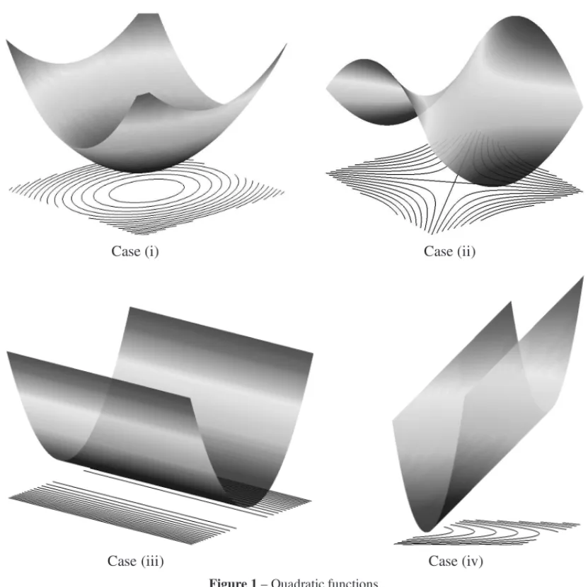
The behavior of a quadratic function depends on the eigenvalues of its Hessian H. Since H is symmetric, it is known thatHhasnreal eigenvalues
µ1≤µ2≤. . .≤µn,
which may be associated withnorthonormal (mutually orthogonal with unit norm) eigenvectors
v1, v2, . . . , vn. There are four cases, represented in Figure 1:
(i) Ifµ1 > 0, thenH is a positive definite matrix, f is strictly convex and its unique
mini-mizer is the unique solution ofH x= −c.
(ii) Ifµ1<0, then infx∈Rn f(x)= −∞, and f(x)→ −∞along the directionv1.
Consider now the cases in which there are null eigenvalues. Let them be µ1 = µ2 =
. . .=µk =0. ThusHis a positive semi-definite matrix.
(iii) IfcTvi =0 for i=1, . . . ,k, then f has ak-dimensional set of minimizers.
(iv) IfcTvi <0 for some i=1, . . . ,k, then f is unbounded below.
In this section, we study the following scheme:
: the class of quadratic functions that are bounded below (cases (i) and (iii) above). A func-tion inhas at least one minimizerx∗. Without loss of generality, the study of algorithmic properties (not the implementation) may assume thatx∗=0, and so the function becomes
f(x)= 1
2x
TH x, with
∇f(x)=H x and f∗ = f(x∗)=0. (2)
O: O(x)= {f(x),∇f(x)} (first order).
τε: Given an initial pointx0∈Rn, two rules will be used in the analysis:
•Absolute error bound: f(x)− f∗≤ε,
•Relative error bound: f(x)− f∗≤ε(f(x0)− f∗).
These rules are not implementable, because they require the knowledge ofx∗, but are very useful in the performance analysis.
Case (i) Case (ii)
Case (iii) Case (iv)
Figure 1– Quadratic functions.
3.1 Steepest descent algorithms
In the first half of the 19thcentury, Cauchy found that the gradient∇f(x)of a function f is the direction of maximum ascent of f fromx, and stated the gradient method. It is the most basic of all optimization algorithms, and its performance is still an active research topic.
Algorithm 3.Steepest descent algorithm (model)
Data:x0∈Rn,ε >0,k=0 WHILExkdoes not satisfyτε
Choose a steplengthλk >0
Steplengths:Each different method for choosing the steplengthsλkdefines a different steepest descent algorithm. Let us describe the two best known choices for the steplengths:
• The Cauchy step, or exact step,
λk=argmin
λ≥0
f(xk−λ∇f(xk)), (3)
the unique minimizer of f along the direction−g withg = ∇f(xk). The steplength is computed by setting∇f(xk−λkg)⊥gand simplifying, which results in
λk= gTg
gTH g. (4)
• The short step:λk<2/µn, a fixed steplength.
Complexity results
Now we study the iteration performance of the steepest descent methods with these two step-length choices for minimizing a strictly convex quadratic function (case (i)). Givenε > 0 and x0∈Rn, we consider thatτεis satisfied at a givenx∈Rnif
f(x)− f∗≤ε (f(x0)− f∗) (relative error bound). (5)
In both cases the algorithm stops in O(Clog(1/ε))iterations, whereC =µn/µ1. At this moment
the following question is open: find a steepest descent algorithm (by a different choice ofλk) with performance O(√Clog(1/ε)). This performance is achieved in practice for “normal
prob-lems” (but not for particular worst case problems) by Barzilai-Borwein and spectral methods, described in [3].
Theorem 1. LetC =µn/µ1≥ 1be the condition number of H . The iteration performance of
the steepest descent method with Cauchy steplength for minimizing f starting at x0 ∈ Rnand with stopping criterion(5)is given by
k≤ C
4 log 1
ε .
Proof. We begin by stating a classical result for the steepest descent step, which is based on the Kantorovich inequality and is proved for instance in [12, p. 238],
f(xk)≤
C
−1
C+1
2
f(xk−1).
Using this recursively, we obtain
f(xk)
f(x0) ≤
C
−1
C+1
2k
=
C
−1
C+1
2CkC
which implies
log
f(xk)
f(x0)
≤ 2kC log C
−1
C+1
C
.
It is known thatt∈ [1,+∞)→tt−+11
t
is an increasing function and that fort>1,
t
−1 t+1
t
≤ lim t→∞
t
−1 t+1
t
= 1
e2.
Consequently
log
f(xk)
f(x0)
≤ 2kC log
1 e2
=−C4k.
Ifτεis not satisfied at an iterationk, then by(5), f(x
k) f(x0) > εor
log(ε) <log
f(xk)
f(x0)
≤ −4kC,
which impliesk< C4log1ε, completing the proof.
Example.In this example we show that the bound obtained in Theorem 1 is sharp, i.e., it cannot be improved. Take the following problem inR2:
f(x)=1
2x TH x
with H=diag(1,C) (i.e. µ1=1, µ2=C).
Assume that the initial point of some iteration has the shapex=(C,1)z, for somez∈R. Then
∇f(x)=(x1,Cx2)=(1,1)Cz.
Computing the steplengthλby(4), we obtainλ=2/(C+1), and then the next iterate will be
x+=(C,1)z− 2C
C+1 (1,1)z= C−1 C+1 (
C,−1)z.
It follows that
f(x+)=
C
−1
C+1
2 f(x),
and this will be repeated on all iterations, with the worst possible performance as in Theorem 1.
Theorem 2.LetC =µn/µ1 ≥1be the condition number of H . The iteration performance of
the steepest descent method with short stepsλk =1/µn, for minimizing f starting at x0 ∈Rn and with stopping criterion(5)is given by
Proof. A simplification in the analysis can be made by diagonalizing the matrixHby using the orthonormal matrix whose columns are the eigenvectors ofH. Thus, we can consider, without loss of generality, thatH =diag(µ1, . . . , µn). Givenx0∈Rn, by the steepest descent algorithm with short steps,
xk =xk−1− 1
µn∇
f(xk−1)=
I− 1
µn H
xk−1.
Thus, for alli=1, . . . ,n,
x k i = 1− µi
µn
x
k−1 i
≤
1−C1
x
k−1 i
.
Consequently, by the definition of f,
f(xk)≤
1−C1
2
f(xk−1).
Proceeding like in the proof of Theorem 1, we obtain
log
f(xk)
f(x0)
≤ 2kC log
lim t→∞
1−1
t t
= 2kC log
1 e
=−C2k.
So, ifτεis not satisfied at an iterationk, thenk< C2log
1
ε
, completing the proof.
Remarks:
• When the short steps 1/µn are used, the result is that fori = 1, . . . ,n,|xki| ≤ √ε|xi0|, fork ≥ C2log(1/ε). Hence not only f(xk) ≤ εf(x0), but alsoxk ≤ √εx0 and
∇f(xk) ≤√ε∇f(x0).
• The diagonalization of H can be made without loss of generality for the performance analysis, as we did in the proof of Theorem 2. This leads to an interesting observation about the constantC, for the case in which there are null eigenvalues (case(iii)). Assuming
thatµ1 = µ2 = . . . =µp = 0, we see that fori = 1, . . . ,p,(∇f(x))i = 0, and the variablesxiremain constant forever having no influence on the performance. The bounds in Theorems 1 and 2 remain valid forC =µn/µp
+1.
3.2 Krylov methods
Krylov space methods are the best possible algorithms for minimizing a quadratic function using only first-order information. Let us describe the geometry of a Krylov space method for the quadratic(2).
• Starting at a pointx0, define the lineV1=x0+θ∇f(x0)|θ∈Rand
x1=argmin x∈V1
f(x)=x0+θ∇f(x0). (P1)
• Second step: take the affine space defined by ∇f(x0) and ∇f(x1), V2 = x0 +
span∇f(x0),∇f(x1)and note that since∇f(x1) = H(x0+θ ∇f(x0)) = H x0+
θ H2x0,
V2=x0+span
H x0,H2x0
and the next iterate will be
x2=argmin x∈V2
f(x). (P2)
This is a two-dimensional problem.
• k-th step: adding∇f(xk−1)to the set of gradients, we construct the set
Vk=x0+span
H x0, . . . ,Hkx0
and the next point will be
xk =argmin x∈Vk
f(x), (Pk)
ak−dimensional problem.
Since∇f(xk)⊥Vkbecause of the minimization, either∇f(xk)=0 and the problem is solved, orVk+1is(k+1)−dimensional. It is then clear thatxnis an optimal solution becauseVn=Rn. This gives us a first performance boundk≤ nfor the Krylov space method. This bound is bad for high-dimensional spaces.
Main question:how to solve (Pk). Without proof (see for instance [15, 20]), it is known that the directions(xk−xk−1)are conjugate, and any conjugate direction algorithm like Fletcher-Reeves [4, 18] solves (Pk) at each iteration with about the same work as in the steepest descent method.
From now on we do a performance analysis of the Krylov space method, with stopping criterion
f(xk)− f∗≤ε (absolute error bound).
A result for the relative error bound will also be discussed in the end of the section. The analysis is quite technical and will result in(16).
Definition 1.Given x0∈Rnand k∈N, define the k-th Krylov space by
Kk=spanH x0,H2x0, . . . ,Hkx0.
ConsiderVk=x0+Kkand define the sequence(xk)by
xk =argmin x∈Vk
f(x). (6)
LetPkbe the set of polynomialsp:R→Rof degreeksuch thatp(0)=1, i.e,
From now on we deal with matrix polynomials, settingt =H.
Lemma 1. A point x ∈Vk if, and only if, x = p(H)x0for some polynomial p∈ Pk. Further-more,
f(x)= 1
2(x
0)TH p(H)2
x0. (8)
Proof. A pointx∈Vkif, and only if,
x=x0+a1H x0+a2H2x0+ · · · +akHkx0= p(H)x0,
wherep∈Pk. Furthermore,
f(x)= 1
2(x
0)T p(H)T
H p(H)x0.
AsHis symmetric, p(H)T
H=H p(H), completing the proof.
Lemma 2.For any polynomial p∈Pk,
f(xk)≤ 1
2(x
0)TH p(H)2
x0.
Proof. Consider an arbitrary polynomial p ∈ Pk. From Lemma 1, the point x = p(H)x0
belongs toVk. As xk minimizes f inVk, we have f(xk)≤ f(x). Using(8)we complete the
proof.
Lemma 3.Let A∈Rn×nbe a symmetric matrix with eigenvaluesλ1, λ2, . . . , λn. If q:R→R is a polynomial, then q(λ1),q(λ2), . . . ,q(λn)are the eigenvalues of q(A).
Proof. AsAis a symmetric matrix, there exists an orthogonal matrix Psuch thatA=P D PT, withD=diag(λ1, λ2, . . . , λn). Ifq(t)=a0+a1t+ · · · +aktk, then
q(H)=a0I +a1P D PT + · · · +ak(P D PT)k =P
a0I+a1D+ · · · +akDk
PT.
Note that
a0I+a1D+ · · · +akDk =diagq(λ1),q(λ2), . . . ,q(λn)
which completes the proof.
3.2.1 Chebyshev Polynomials
Definition 2.The Chebyshev polynomial of degree k, Tk : [−1,1] →R, is defined by
Tk(t)=coskarccos(t).
The next lemma shows thatTk is, in fact, a polynomial (even though it does not look like one).
Lemma 4.For all t ∈ [−1,1], T0(t)=1and T1(t)=t . Furthermore, for all k≥1,
Tk+1(t)=2t Tk(t)−Tk−1(t).
Proof. The first statements follow from the definition. In order to prove the recurrence rule, considerθ: [−1,1] → [0, π], given byθ (t)=arccos(t). Thus,
Tk+1(t)=cos(k+1)θ (t)=coskθ (t)cosθ (t)−sinkθ (t)sinθ (t)
and
Tk−1(t)=cos(k−1)θ (t)=coskθ (t)cosθ (t)+sinkθ (t)sinθ (t).
But cos kθ (t)
=Tk(t)and cosθ (t)=t. So,
Tk+1(t)+Tk−1(t)=2t Tk(t),
completing the proof.
Lemma 5.If Tk(t)=aktk+ · · · +a2t2+a1t+a0, then ak=2k−1. Furthermore,
(i) If k is even, then a0=(−1) k
2 and a2j
−1=0, for all j =1, . . . ,k2;
(ii) If k is odd, then a1=(−1) k−1
2 k and a2j =0, for all j=0,1, . . . ,k−1
2 .
Proof. We prove by induction. The results are trivial fork = 0 and k = 1. Suppose that the results hold for all natural number less than or equal tok. Using the induction hypothesis, consider
Tk(t)=2k−1tk+ · · · +a1t+a0 and Tk−1(t)=2k−2tk−1+ · · · +b1t+b0.
By Lemma 4,
Tk+1(t)=2t(2k−1tk+ · · · +a1t+a0)−(2k−2tk−1+ · · · +b1t+b0), (9)
leading to the first statement. Suppose that(k+1)is even. Thenkis odd and(k−1)is even. Thus, by induction hypothesis,Tk has only odd powers oftandTk−1has only even powers. In
this way, by(9),Tk+1has only even powers oft. Furthermore, its independent term is
−b0= −(−1) k−1
2 =(−1)
On the other hand, if(k+1)is odd, thenkis even and(k−1)is odd. Again by the induction hypothesis,Tk only has even powers oft andTk−1has only odd powers. Thus by(9),Tk+1has
only odd powers oft. Furthermore, its linear term is
2t a0−b1t=2t(−1) k
2 −(−1)
k−2
2 (k−1)t =(−1)
k
2(k+1)t,
completing the proof.
The next lemma discusses a relationship between a Chebyshev polynomial of odd degree and polynomials of the setPk, defined in(7).
Lemma 6.Consider L >0and k∈N. Then there exists p∈Pk such that, for all t ∈ [0,L],
T2k+1
√t
√
L
=(−1)k(2k+1)
√
t
√
L p(t).
Proof. By Lemma 5, for allt∈ [−1,1], we have
T2k+1(t)=t
22kt2k+ · · · +(−1)k(2k+1),
where the polynomial in parentheses has only even powers oft. So, for allt ∈ [0,L],
T2k+1
√t √ L = √ t √ L
22k t
L k
+ · · · +(−1)k(2k+1)
.
Defining
p(t)= 1 (−1)k(2k+1)
22k
t L
k
+ · · · +(−1)k(2k+1)
,
we complete the proof.
3.2.2 Complexity results
Now we present the main result about the performance of Krylov methods for minimizing a convex quadratic function. This result is based on [19, Thm. 3, p. 170].
We use the matrix norm defined by
A =sup{Ax | x =1} =max{|λ| |λis an eigenvalue ofA}. (10)
Theorem 3. Letµn be the largest eigenvalue of H and consider the sequence(xk)defined by
(6). Then for k∈N
f(xk)− f∗≤ µnx
0 −x∗2
2(2k+1)2 , (11)
and f(xk)− f∗≤ε is satisfied for
k≤ 1 √ 8 √µ
nx0−x∗ √
ε
Proof. Without loss of generality, assume that x∗ = 0. By Lemma 2, for all polynomial p∈Pk,
f(xk)≤ 1
2(x
0)TH
p(H)2x0≤ 1 2x
0 2 H p(H)2
. (13)
But, from Lemma 3 and(10),
H
p(H)2
=max µi
p(µi) 2
|µi is an eigenvalue ofH
.
Considering the polynomialp∈Pk given in Lemma 6 and using the fact that all eigenvalues of
Hbelong to(0, µn], we have
H
p(H)2
≤ max t∈[0,µn]
t
p(t)2
= µn
(2k+1)2tmax
∈[0,µn]
T22k+1 √t
õ n
≤ µn
(2k+1)2,
(14)
proving(11). Ifτε is not satisfied at an iterationk, then f(xk) > εand consequently
ε < µnx
0 2
2(2k+1)2 <
µnx02 8k2
which implies(12)and completes the proof.
Performance of the method for the relative error bound:A similar analysis forτεgiven by
(5), also using Chebyshev polynomials, can be done using the condition numberC. This is done
in [14, 23], and the result is
k≤ √ C 2 log 2 ε =O √ C log 1 ε ,
clearly better than the best performance of the steepest descent algorithm for the steplength rules studied above, and for reasonable values ofµ1, better than(12).
Complexity bound. The Krylov space methods uses at each iteration all the information gath-ered in the previous steps, and hence it seems to be the best possible algorithm based on first order information. In fact, Nemirovskii & Yudin [14] prove that no algorithm using a first order oracle can have a performance more than twice as good as the Krylov space method.
For methods based on accumulated first order information there is a negative result described by Nesterov [15, p. 59]: he constructs a quadratic problem (which he calls “the worst problem in the world”) for which such methods need at least
k= 3
32
õ
nx0−x∗ √
ε (15)
iterations to reachτε.
We conclude that the best performance for a first order method must be between the bounds(12)
and(15). So the complexity of the scheme is
4 CONVEX DIFFERENTIABLE FUNCTIONS: THE BASIC ALGORITHM
In this section we study the performance of algorithms for the unconstrained minimization of differentiable convex functions. Quadratic functions are a particular case, and hence the perfor-mance bounds for first order algorithms will not be better than those found in the former section.
The role played byµn in quadratic functions will be played by a Lipschitz constant L for the gradient of f (indeed, for a quadratic function the largest eigenvalue is a Lipschitz constant for the gradient), and we shall see that there are optimal algorithms, i.e., algorithms with the performance given by(16)withµnreplaced byL. These algorithms were developed by Nesterov [15], and are also studied in our papers [7, 8].
Consider the scheme(,O, τε)where
: the class of minimization problems of a convex continuously differentiable function f, with a Lipschitz constantL >0 for the gradient. It means that for allx,y∈Rn,
∇f(x)− ∇f(y) ≤Lx−y. (17)
O: O(x)= {f(x),∇f(x)} (first order)
τε: defined by f(x)− f∗≤εwherex∗is a solution of the problem and f∗= f(x∗).
Simple quadratic functions. The following definition will be useful in our development: we shall call “simple” a quadratic functionφ : Rn → Rwith∇2φ (x)=γI,γ ∈R,γ > 0. The following facts are easily proved for such functions:
• φ (·)has a unique minimizerv∈Rn(which we shall refer as thecenterof the quadratic), and the function can be written as
x∈Rn→φ (v)+γ
2x−v
2. (18)
• Givenx∈Rn,
v=x− 1
γ∇φ (x), (19)
and
φ (x)−φ (v)= 1
2γ∇φ (x)
2.
(20)
4.1 The algorithm
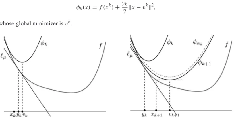
We begin by summarizing the geometrical construction at an iterationk, represented in Figure 2. The iteration starts with two pointsxk, vk∈Rnand a simple quadratic function
φk(x)= f(xk)+
γk 2 x−v
k 2,
whose global minimizer isvk.
Figure 2–The mechanics of the algorithm.
A pointyk =xk+α(vk−xk)is chosen betweenxk andvk. The choice ofαis a central issue, and will be discussed later. All the action is centered onyk, with the following construction:
• Take a gradient step fromyk, generatingxk+1.
• Define a linear approximation of f(·)
x ∈Rn→ℓ(x)= f(yk)+ ∇f(yk)T(x−yk).
• Compute a valueα ∈ (0,1), and define φα(x) = αℓ(x)+(1−α)φk(x), with Hessian
γk+1I = ∇2φα(x)=(1−α)γkI, and letvk+1be the minimizer of this simple quadratic. The iteration is completed by defining
φk+1(x)= f(xk+1)+
γk+1
2 x−v k+1
2.
Now we state the algorithm.
Algorithm 4.
Data:x0∈Rn,v0=x0,γ0=L,k=0 REPEAT
Setyk =xk+αk(vk−xk) Compute f(yk)andg= ∇f(yk)
Updates
xk+1=yk−g/L (steepest descent step)
γk+1=(1−αk)γk
For the analysis define
x→φk(x)= f(xk)+γ2kx−vk2 x→ℓ(x)= f(yk)+gT(x−yk)
x→u(x)= f(yk)+gT(x−yk)+ L2x−yk2 x→φαk(x)=αkℓ(x)+(1−αk)φk(x)
vk+1=argminφαk(·)=v k
− αk
γk+1
g
k=k+1.
4.1.1 Analysis of the algorithm
The most important procedure in the algorithm is the choice of the parameter αk, which then determinesykat each iteration. The choice ofαkis the one devised by Nesterov in [15, Scheme (2.2.6)]. Instead of “discovering” the values for these parameters, we shall simply adopt them and show their properties.
Once ykis determined, two independent actions are taken:
(i) A steepest descent step fromykcomputesxk+1.
(ii) A new simple quadratic is constructed by combiningφk(·)and the linear approximation
ℓ(·)of f(·)aboutyk:
φαk(x)=αkℓ(x)+(1−αk)φk(x).
Our scope will be to prove two facts:
• At any iterationk,φ∗α
k ≥ f(x k+1).
• For allx∈Rn,φ
k+1(x)− f(x)≤(1−αk)(φk(x)− f(x)).
From these facts we shall conclude that f(xk)→ f∗ with the same speed asγk → 0, which easily leads to the desired performance result.
The first lemma shows our main finding about the geometry of these points. All the action happens in the two-dimensional space defined byxk, vk, vk+1. Note the beautiful similarity of the triangles in Figure 3.
Lemma 7.Consider the sequences generated by Algorithm 4. Then for k ∈N,
g
xk yk vk
vk+1 xk+1
Figure 3–Geometric properties of the steps.
Proof. By the algorithm, we know thatLα2k =γk+1, and
αk(vk+1−xk)=αk
vk−xk− αk
γk+1
g
=αk(vk −xk)−
αk2 γk+1
g
=αk(vk −xk)− 1 Lg
=yk−xk− 1 Lg
=xk+1−xk,
completing the proof.
Lemma 8.Consider the sequences generated by Algorithm 4. Then for k∈N,
f(yk)≤φαk(v k).
Proof. By the definition ofφαk,
φαk(v k)
=αkℓ(vk)+(1−αk)φk(vk).
But,φk(vk)= f(xk)≥ℓ(xk). Using this, the definition ofℓand the fact thatαk ∈ (0,1), we have
φαk(v k)
≥αkℓ(vk)+(1−αk)ℓ(xk)
=αk
f(yk)+gT(vk−yk)+(1−αk)
f(yk)+gT(xk −yk)
= f(yk)+gTαk(vk−yk)+(1−αk)(xk−yk)
. (21)
By the definition ofykin the algorithm,vk−yk =(1−αk)(vk−xk)andxk−yk = −αk(vk−xk).
Lemma 9.Consider the sequences generated by Algorithm 4. Then for k ∈N,
f(xk+1)≤u(xk+1)≤φαk(v k+1)
=φα∗
k, (22)
φk+1(·)≤φαk(·). (23)
Proof. The first inequality follows trivially from the convexity of f and the definition ofu.
Sincexk+1andvk+1 are respectively global minimizers ofu(·)andφαk(·), we have from(18) that, for allx ∈Rn,
u(x)=u(xk+1)+ L
2x−x k+1
2 and φαk(x)=φα∗k+
γk+1
2 x−v k+1
2. (24)
As f(yk)=u(yk)and, from the last lemma,u(yk)≤φαk(v
k), we only need to show that
u(yk)−u(xk+1)=φαk(v k)
−φα∗
k.
The construction is shown in Fig. 3: since, by Lemma 7,xk+1=xk+αk(vk+1−xk),
yk−xk+1=αk(vk−vk+1).
Using this,(24)and the fact that by construction,αk2= γk+1
L , we obtain
u(yk)−u(xk+1)= Lα
2 k 2 v
k
−vk+12= γk+1
2 v k
−vk+12=φαk(v k)
−φα∗
k,
proving the second inequality of(22).
By construction,
φk+1(x)= f(xk+1)+
γk+1
2 x−v k+1
2.
Comparing to(24)and using the fact that f(xk+1)≤φα∗
k, we get(23), completing the proof.
Lemma 10.For any x∈Rnand k∈N,
φk(x)− f(x)≤
γk
γ0
(φ0(x)− f(x)) . (25)
Proof. By the definition ofφαk and the fact thatℓ(x)≤ f(x), for allx∈R n,
φαk(x)≤αkf(x)+(1−αk)φk(x).
Subtracting f(x)in both sides, using(23)and the definition ofγk+1, we have
φk+1(x)− f(x)≤φαk(x)− f(x)
≤(1−αk)(φk(x)− f(x))
=γk+1
γk
(φk(x)− f(x)).
4.1.2 Complexity
The following lemma was proved by Nesterov [15, p. 77] with a different notation.
Lemma 11.Consider the sequence(γk)generated by Algorithm 4, i.e., givenγ0>0,
γk+1=(1−αk)γk, Lαk2=γk+1.
Then, for k∈N,γk≤4L/k2.
Proof. Asαk=√γk+1/L,
γk+1=
1−√1
L
√γ k+1
γk.
Thus, the result follows directly from [7, Lemma 10].
Theorem 4.Consider the sequences generated by Algorithm 4 and assume that x∗is an optimal solution. Then for k∈N,
f(xk)− f∗≤ 4L k2x
∗−x
02, (26)
and f(xk)− f∗≤ε is satisfied for
k≤
2
√
Lx0−x∗
√
ε
. (27)
Proof. From Lemma 10,(25)holds in particular atx∗,
φk(x∗)− f∗≤
γk
γ0
φ0(x∗)− f∗.
Using the fact that f(xk)=φk(vk)≤φk(x∗)and the definition ofφ0, we get,
f(xk)− f∗≤ γk
γ0
f(x0)+
γ0
2x
∗−x02
− f∗. (28)
Sincex∗is a minimizer of the convex function f,
f(x0)− f∗≤ L
2x ∗−x0
2.
Applying this and the result of Lemma 11 in(28),
f(xk)− f∗≤ 2L(L+γ0)
γ0k2
x∗−x02.
Asγ0 = L, we have (26). If τε is not satisfied at an iterationk, then f(xk)− f∗ > ε and
consequently
ε < 4L
k2x
∗−x
02,
So, the iteration performance of Algorithm 4 is
k=√Lx0−x∗O1/√ε,
which corresponds to the complexity (16) for quadratic performance. Then, the algorithm is optimal.
5 CONVEX DIFFERENTIABLE FUNCTIONS: ENHANCED ALGORITHMS
The algorithm presented in the former section may be extended in several ways: the need for a previous knowledge of a Lipschitz constant L may be eliminated, a strong convexity constant akin to the smallest eigenvalue in the quadratic case may be used, and the algorithm may be extended to problems constrained to so-called simple sets. These extensions are treated in our paper [8] and in references therein.
In this section we state the extension of the basic algorithm to problems with simple constraints, without proofs. Consider the scheme(,O, τε)where
: the class of problems
minimize f(x)
subject to x∈,
where ⊂ Rn is a closed convex set and f : Rn → R is convex and continuously
differentiable, with a Lipschitz constantL > 0 for the gradient. We assume thatis a “simple” set, in the following sense: given an arbitrary pointx∈Rn, an oracle is available
to computeP(x)=argmin
y∈
x−y, the orthogonal projection onto the set.
O: O(x)= {f(x),∇f(x),P(x)}.
τε: defined by f(x)− f∗≤εwherex∗is a solution of the problem and f∗= f(x∗).
We now state the basic algorithm for constrained problems, without proofs. We keep in the statement the definition of the functions used in the analysis made in [8].
Algorithm 5.
Data: x0∈,v0=x0,γ0=L,k=0 REPEAT
Computeα∈(0,1)such thatLα2=(1−α)γk yk =xk+α(vk−xk)
Compute f(yk)andg= ∇f(yk)
Updates
xk+1= P(yk−g/L) (projected steepest descent step)
For the analysis define
x→φk(x)= f(xk)+γ2kx−vk2 x→ℓ(x)= f(yk)+gT(x−yk)
x→u(x)= f(yk)+gT(x−yk)+L2x−yk2 x→φαk(x)=αkℓ(x)+(1−αk)φk(x)
vk+1=argmin x∈
φαk(x)=P
vk− αk
γk+1
g
k=k+1.
Consider the sequences generated by Algorithm 5. Then, as proved in [8, Thm. 2.6], at any iterationkbefore stopping,
ε≤ f(xk)− f∗≤ 4 k2
f(x0)− f∗+
L 2 x
∗−x
02
.
and hence
k≤ √2
ε
f(x0)− f∗+
L 2 x
∗−x02 1/2
.
This expression is similar to(27). In fact, ifx∗is a global minimizer, then
f(x0)− f∗≤ L 2 x
∗−x02
may be introduced in the last expression, retrieving(27).
Estimations of the Lipschitz constant. Both Algorithms 4 and 5 and the algorithms discussed by Nesterov in [15, Chapter 2] make explicit use of a Lipschitz constantLfor the function gra-dient. In [16], Nesterov describes a method for a more general problem, easily applied to the situations studied in this paper. This method includes a scheme for estimating the Lipschitz con-stant. In [7, 8], the authors eliminate the use ofLat the cost of an extra imprecise line search, and obtain an algorithm which keeps the optimal complexity properties and also inherits the global convergence properties of the steepest descent method for general continuously differentiable optimization. Besides this, the algorithm takes advantage of the knowledge of the strong convex-ity constant for the function and develop in [7] an adaptive procedure for estimating it. In another context – constrained minimization of non-smooth homogeneous convex functions – Richt´arik [21] uses an adaptive scheme for guessing bounds for the distance between a pointx0 and an
optimal solutionx∗. This bound determines the number of subgradient steps needed to obtain a desired precision.
6 CONCLUSIONS
In this paper we described what we believe to be the basic results in the study of algorithm per-formance and problem complexity for the minimization of convex functions, both unconstrained and with simple constraints.
Algorithms with proved low worst-case performance are not necessarily efficient for practical problems. Khachiyan’s algorithm [10] for linear programming is very inefficient, but had a great impact on the development of both continuous and discrete optimization. Karmarkar’s algorithm [9] for linear programming improved Khachiyan’s performance bound, and his bound was again improved later (see [6]). The effort to improve complexity led to better algorithms, which are nowadays used for solving large scale linear and quadratic in many domains. In fact, the largest linear programming problem treated up to now had 1.1 billion variables and 380 million con-straints, solved by Gondzio & Grothey [5] using an interior point algorithm.
The conjugate gradient algorithm (Krylov space method) has optimal performance for quadratic problems, but its extension to more general problems is not straightforward. It was superseded by quasi-Newton methods, which are more efficient for non-quadratic problems, but coincide with it in the convex quadratic case. Note that the conjugate gradient method was not motivated by the complexity study, which came later.
Accelerated gradient methods are now in the phase of development, and we are not aware of any extensive comparison with classical algorithms. Research in this field is presently very active, and it is not clear to what classes of problems this approach will be applied and which methods will be the winners in practical applications to large-scale problems.
REFERENCES
[1] AUSLENDERA & TEBOULLEM. 2006. Interior gradient and proximal methods for convex and conic optimization.SIAM Journal on Optimization,16(3): 697–725.
[2] BECKA & TEBOULLEM. 2009. A fast iterative shrinkage-thresholding algorithm for linear inverse problems.SIAM J. Img. Sci.,2(1): 183–202, March.
[3] BIRGINEG, MART´INEZJM & RAYDANM. 2009. Spectral Projected Gradient Methods. In C.A. Floudas and P.M. Pardalos, editors,Encyclopedia of Optimization, pages 3652–3659. Springer.
[4] FLETCHERR & REEVESCM. 1964. Function minimization by conjugate gradients.Computer J.,7: 149–154.
[5] GONDZIOJ & GROTHEYA. 2006. Solving nonlinear financial planning problems with 109decision variables on massively parallel architectures. In M. Costantino and C. A. Brebbia, editors, Computa-tional Finance and its Applications II, WIT Transactions on Modelling and Simulation, 43, volume 43. WIT Press.
[6] GONZAGACC. 1992. Path-following methods for linear programming.SIAM Review,34(2): 167– 224.
[8] GONZAGACC, KARASEW & ROSSETTODR. 2013. An optimal algorithm for constrained differ-entiable convex optimization.SIAM Journal on Optimization,23(4): 1939–1955.
[9] KARMARKARN. 1984. A new polynomial time algorithm for linear programming.Combinatorica, 4: 373–395.
[10] KHACHIYANLG. 1979. A polynomial algorithm for linear programming.Doklady Akad. Nauk USSR, 244: 1093–1096. Translated in Soviet Math. Doklady 20: 191–194.
[11] LAN G, LUZ & MONTEIRORDC. 2011. Primal-dual first-order methods with O(1/ε) iteration-complexity for cone programming.Mathematical Programming,126(1): 1–29.
[12] LUENBERGERDG & YEY. 2008.Linear and Nonlinear Programming. Springer, New York, third edition.
[13] MONTEIRORDC, ORTIZC & SVAITERBF. 2012. An adaptive accelerated first-order method for convex optimization. Technical report, School of ISyE, Georgia Tech, July.
[14] NEMIROVSKIAS & YUDINDB. 1983.Problem Complexity and Method Efficiency in Optimization. John Wiley, New York.
[15] NESTEROVY. 2004.Introductory Lectures on Convex Optimization. A basic course. Kluwer Aca-demic Publishers, Boston.
[16] NESTEROVY. 2013. Gradient methods for minimizing composite objective function.Mathematical Programming,140(1): 125–161.
[17] NESTEROVY & POLYAKBT. 2006. Cubic regularization of Newton method and its global perfor-mance.Mathematical Programming,108: 177–205.
[18] NOCEDALJ & WRIGHTSJ. 2006.Numerical Optimization. Springer Series in Operations Research. Springer-Verlag, 2nd edition.
[19] POLYAKBT. 1987.Introduction to Optimization. Optimization Software Inc., New York.
[20] RIBEIROAA & KARASEW. 2013.Otimizac¸ ˜ao Cont´ınua: aspectos te ´oricos e computacionais. Cen-gage Learning. In Portuguese.
[21] RICHTARIK´ P. 2011. Improved algorithms for convex minimization in relative scale.SIAM Journal on Optimization,21(3): 1141–1167.
[22] ROSSETTODR. 2012.T´opicos em m´etodos ´otimos para otimizac¸ ˜ao convexa. PhD thesis, Department of Applied Mathematics, University of S˜ao Paulo, Brazil. In Portuguese.
[23] SHEWCHUKJR. 1994. An introduction to the conjugate gradient method without the agonizing pain.