Evaluation of the flux gradient technique for measurement of ozone surface fluxes over snowpack at Summit, Greenland

(1)

AMTD

4, 1021–1059, 2011

Evaluation of the flux gradient technique

for measurement

F. Bocquet et al.

Title Page Abstract Introduction Conclusions References Tables Figures

◭ ◮

Back Close Full Screen / Esc

Printer-friendly Version Interactive Discussion

Discussion

P

a

per

|

Dis

cussion

P

a

per

|

Discussion

P

a

per

|

Discussio

n

P

a

per

|

Atmos. Meas. Tech. Discuss., 4, 1021–1059, 2011 www.atmos-meas-tech-discuss.net/4/1021/2011/ doi:10.5194/amtd-4-1021-2011

Atmospheric Measurement Techniques Discussions

This discussion paper is/has been under review for the journal Atmospheric Measure-ment Techniques (AMT). Please refer to the corresponding final paper in AMT

if available.

Evaluation of the flux gradient technique

for measurement of ozone surface fluxes

over snowpack at Summit, Greenland

F. Bocquet1,*, D. Helmig1, B. A. Van Dam1, and C. W. Fairall2

1

Institute of Arctic and Alpine Research, University of Colorado at Boulder, UCB 450, Boulder, CO 80309, USA

2

Earth System Research Laboratory, NOAA,

Boulder, Colorado USA, 325 Broadway, Boulder, CO 80303, USA *

now at: Cooperative Institute for Research in Environmental Sciences, University of Colorado at Boulder, UCB 216, Boulder, CO 80309, USA

Received: 19 January 2011 – Accepted: 21 January 2011 – Published: 14 February 2011 Correspondence to: D. Helmig (detlev.helmig@colorado.edu)

(2)

AMTD

4, 1021–1059, 2011

for measurement

F. Bocquet et al.

◭ ◮

Discussion

P

a

per

|

Dis

cussion

P

a

per

|

Discussion

P

a

per

|

Discussio

n

P

a

per

|

Abstract

A multi-step procedure for investigating ozone surface fluxes over polar snow by the tower gradient method was developed and evaluated. These measurements were then used to obtain four months of turbulent ozone flux data at the Summit research camp located in the center of the Greenland ice shield. Turbulent fluxes were determined by

5

the aerodynamic gradient method incorporating tower measurements of (a) ozone gra-dients measured by commercial ultraviolet absorption analyzers, (b) ambient tempera-ture gradients using aspirated thermocouple sensors, and (c) wind speed gradients de-termined by cup anemometers. All gradient instruments were regularly inter-compared by bringing sensors or inlets to the same measurement height. The developed protocol

10

resulted in an uncertainty on the order of 0.1 ppbv for 30-min averaged ozone gradients that were used for the ozone flux calculations. This protocol facilitated a lower sensi-tivity threshold for the ozone flux determination of₋8_×10−3µg m−2s−1, respectively

∼0.01 cm s−1for the ozone deposition velocity for typical environmental conditions en-countered at Summit. Uncertainty in the 30-min ozone exchange measurements

(eval-15

uated by the Monte Carlo statistical approach) was on the order of 10−2cm s−1. This

uncertainty typically accounted to _∼20–100% of the ozone exchange velocities that

were determined. These measurements are among the most sensitive ozone depo-sition determinations reported to date. This flux experiment, deployed at Summit for a period of four months, allowed for measurements of the relatively low ozone uptake

20

rates encountered for polar snow, and thereby the study of their environmental and seasonal dependencies.

1 Introduction

Gas flux to the surface is commonly described by an analogy to electrical resistances

taking into account physical and chemical processes aff_{ecting the flux. In chemical}

25

(3)

AMTD

4, 1021–1059, 2011

for measurement

F. Bocquet et al.

◭ ◮

Discussion

P

a

per

|

Dis

cussion

P

a

per

|

Discussion

P

a

per

|

Discussio

n

P

a

per

|

with the surfaces (e.g., snow, ice, sea-ice) is typically represented by a surface resis-tance (R=_v−1

d ,vd=deposition velocity). For snow, an ozone surface resistance value

of 2000 s m−1 is commonly used, and this value is kept constant throughout the day

and the year (Ganzeveld and Lelieveld, 1995; Lamarque et al., 2005; Rotman et al., 2004). Recent research has provided a plethora of evidence for an active

photochem-5

istry in the snowpack (Grannas et al., 2007). Ozone behavior in the snow has been one of the most intensely studied subjects. Ozone in the polar snowpack has been found to undergo depletion that follows both the diurnal and seasonal cycle in solar radiation (Helmig et al., 2007a). These observations suggest that ozone surface fluxes should vary similarly with time of day and season. Previous ozone flux measurements

10

over polar snow have not been able to capture this behavior, likely due to the lack of measurement sensitivity and required long-term observations.

Regener (1957), Galbally (1968), and Aldaz (1969) were among the first researchers to study ozone uptake to the Earth’s surface. A review of atmosphere-surface exchange measurement techniques used in the subsequent 20 years was given by Dabberdt et

15

al. (1993). Table 1 in the Supplement Materials provides a summary of experimental ozone flux techniques from our review of more than 120 published papers on ozone de-position and gas exchange. Ozone dede-position results span a wide range. The largest

ozone exchange velocities (ozone ve; please note that in this paper we will use the

notation of “ozone exchange velocity”, rather than “ozone deposition velocity”, to avoid

20

use of negative velocity values), on the order of 2 cm s−1 have been measured over

vegetation. In comparison, snow and water appear to be the most inert surfaces to-wards ozone.

The overview in the Supplement also lists the diff_{erent types of experimental}

methods, their application areas, and measured rates of ozone surface

deposi-25

tion/exchange. Eddy covariance is the most popular flux method (_∼65%), followed

by the profile/tower gradient method (∼26%), and studies relying on the box/chamber

(4)

AMTD

4, 1021–1059, 2011

for measurement

F. Bocquet et al.

◭ ◮

Discussion

P

a

per

|

Dis

cussion

P

a

per

|

Discussion

P

a

per

|

Discussio

n

P

a

per

|

A total of 12 studies have investigated ozone flux over snow. Galbally and Allison (1972) were the first ones who measured ozone fluxes over old and fresh snow sur-faces at Mt Buller, Australia, and at Mawson, Antarctica. These authors determined vertical ozone gradients using a modified Ehmert potassium iodide ozone sensor. Es-timated errors in the concentration measurement for the flux determination were

re-5

ported to be on the order of_±1 ppbv (Galbally and Allison, 1972). Later on, Colbeck

and Harrison (1985) estimated that “errors in determining individual ozone deposition velocities [to seasonal snow over grassland] are around 30%, the largest contribution to the error being due to the standard error in ozone gradient.” The ozone monitor used in the Colbeck and Harrison (1985) study was a chemiluminescence sensor

us-10

ing ethylene as the reactant that was reported to have a measurement precision of

±1 ppbv. An eddy correlation-based method using a 15-Hz chemiluminescence ozone

monitor reacting with eosin-y was used to measure ozone fluxes over seasonal snow at a subalpine forest site. There was no mentioning of the precision for this measurement (Stocker et al., 1994; Zeller and Hehn, 1996; and Zeller and Nikolov, 2000).

15

While there is a large scatter in measured ozoneve, particularly over snow, a majority of the flux measurement results fall within the range of 0.01–0.1 cm s−1 (Helmig et al., 2007b). Despite this relatively low surface uptake rate, ozone deposition to snow is an important sink for lower atmosphere ozone levels and the oxidative capacity of the

atmosphere over snow. This eff_{ect is due to the relative weakness of other chemical}

20

processes determining the ozone budget, in particular over polar snow (Helmig et al., 2007b).

In this paper we present research aimed at characterizing and improving the sensi-tivity of ozone flux determination by the gradient method, also known as the gradient profile method, and results from field measurements of ozone exchange over the polar

25

(5)

AMTD

4, 1021–1059, 2011

for measurement

F. Bocquet et al.

◭ ◮

Discussion

P

a

per

|

Dis

cussion

P

a

per

|

Discussion

P

a

per

|

Discussio

n

P

a

per

|

amount of eff_{ort was dedicated towards the characterization and optimization of the}

instrument performance.

2 Study site and measurements

These flux experiments were performed at the Summit Environmental Observatory, in the dry-snow zone of the Greenland ice sheet (72◦34′N, 38◦29′W, elevation 3208 m),

5

during 22 March–14 August 2004 (day of the year (DOY) 82–227). The surface

sur-rounding the site is smooth with average surface slopes typically less than 0.005◦.

The relatively flat area at Summit provides a homogenous fetch in all directions, which makes it an excellent site for tower-based flux measurements.

The 12-m flux tower was located _∼250 m south (upwind) of the camp buildings in

10

the “Clean Air Sector”. Ozone, air temperature, and wind speed were measured at three heights of 0.75, 2 and 10 m (Fig. 1; also see Fig. 1 in Helmig et al., 2007a for a schematic diagram of the Summit Flux Facility). Note that the actual sampling heights changed over the course of the study due to the accumulation of new snow. The change in the sensor height was monitored with an ultra-sonic distance sensor

15

(model SR 50, Campbell Scientific Instruments, Logan, UT). Air temperature was mea-sured by type E thermocouple wires mounted into aspirated radiation shields (model 43408, R.M. Young, Traverse City, MI). Temperature gradients were determined di-rectly by wiring thermocouples from two adjacent measurement heights in series. Wind speed was measured with cup anemometers (model 010C, Met One Instruments,

20

Grants Pass, OR). These sensors were mounted on cross arms pointing south of the tower, into the dominating wind direction. Incoming and reflected solar radiation were recorded by two pyranometers (model LiCor 200X, Campbell Scientific Instruments, Logan, UT). Wind speed and temperature sensors were subjected to inter-comparison calibrations on three occasions during the study (beginning, middle and end of the

25

(6)

AMTD

4, 1021–1059, 2011

for measurement

F. Bocquet et al.

◭ ◮

Discussion

P

a

per

|

Dis

cussion

P

a

per

|

Discussion

P

a

per

|

Discussio

n

P

a

per

|

A brief overview of environmental conditions encountered at Summit during the field period is presented in Fig. 2. Air temperature (at 2 m height) (Fig. 2a) increased quite

significantly during the campaign, from_{∼ −}45◦C in spring to maxima of _{∼ −}5◦C

dur-ing late summer. Interestdur-ingly, the amplitude in diurnal temperature variation is larger

during the spring (up to ∼30◦C) than during the summer (∼20◦C). Furthermore, the

5

temperature gradient (2–0.75 m) shifted from being mostly positive (i.e., thermally sta-ble) to alternating between positive and negative on a diurnal basis (i.e., thermally stable at night and unstable during daytime). This change in atmospheric stability from spring to summer is typical for this environment, and has been well documented (Cullen, 2003; Cohen et al., 2007). Wind speed (at 2 m height) (Fig. 2b) averaged

10

around 4.6 m s−1 throughout the period, with increasing frequency of episodes with

winds reaching _∼10 m s−1 as the summer approached. The solar radiation record

(Fig. 2c) reflects the seasonal change in the solar zenith angle from spring to sum-mer. At the beginning of the study period, incoming solar radiation ranged from 0–

400 W m−2. Solar irradiance increased to a range of 50–700 W m−2 at the summer

15

solstice. The net shortwave radiation (incoming minus reflected shortwave radiation)

displays a similar behavior, with minimum values of_∼40 W m−2at the beginning of the

study, and maxima of∼80 W m−2around the summer solstice.

Surface ozone levels at Summit are remarkably high, typically falling within a range of 40–60 ppbv, with an annual median value of 47.5 ppbv (Helmig et al., 2007c). These

20

relatively high ozone concentrations at Summit are due to the elevation of Summit and both the high frequency of ozone transport originating in the upper troposphere, and to occurrences of pollution transport events in the summer (Helmig et al., 2007d). Ozone mixing ratios during this measurement period (Fig. 2d) reflect this behavior, and varied

from 30 to 60 ppbv, with occasional peaks up to_∼70 ppbv.

(7)

AMTD

4, 1021–1059, 2011

for measurement

F. Bocquet et al.

◭ ◮

Discussion

P

a

per

|

Dis

cussion

P

a

per

|

Discussion

P

a

per

|

Discussio

n

P

a

per

|

3 Ozone flux gradient method

3.1 Aerodynamic gradient method

The choice for using the aerodynamic tower gradient method was motivated by the availability of commercial sensors for all required measurements. The aerodynamic tower gradient method is based on the generally accepted micrometeorological

sim-5

ilarity theory (i.e., diff_{usion coe}ffi_{cients for momentum, heat, water vapor and trace}

gases are assumed to be the same). The un-modified aerodynamic method is only valid for neutral stability (for a Richardson numberRi, of 0_±0.01), but empirical func-tions for near-unstable (−0.1<Ri<−0.01) and near-stable (+_0.01_<_Ri_<+_0.1)

condi-tions can be applied to extend the use of the method to a wider range of encountered

10

atmospheric situations (Oke, 1987). In addition, the method requires steady state con-ditions over the averaging time and constant fluxes with height over the measurement interval.

Despite these requirements, the method is relatively simple to use, as it involves measurements of wind speed, air temperature, and ozone mixing ratio at a minimum of

15

two heights. In our case, measurements were conducted at three heights on the 12-m tower, i.e. at 0.75, 2 and 10 m. Ozone monitors record the ozone mixing ratio in unit of parts per billion volume (ppbv), which needs to be converted to an ozone mass per unit volume scale (µg m−3) following

O3(µg·m−3)=

(O₃(ppbv).1000)_×48(g_·mol−1)_×P(Pa)

8.314(J·K−1_·_mol−1

)×(T(◦_C)+₂₇₃_.₁₅₎ (1)

20

where 48 g mol−1 is the molecular weight for ozone O₃, 8.314 J◦C−1mol−1 is the

uni-versal gas constant, andP andT are the measured ambient pressure and temperature

in Pa and◦C, respectively.

The flux of an entity, e.g., ozone, is equated to the product of the concentration

gradient of the entity and the eddy diff_{usivity function characterizing the atmosphere}

(8)

AMTD

4, 1021–1059, 2011

for measurement

F. Bocquet et al.

◭ ◮

Discussion

P

a

per

|

Dis

cussion

P

a

per

|

Discussion

P

a

per

|

Discussio

n

P

a

per

|

transporting that entity (Oke, 1987):

FO₃=−k2zr2( ∆_u

∆_z_u· ∆_O₃

∆_z_O

3

) (2)

where k is the Van Karman constant (=_0.4), _z_r _{is the reference height (also known}

as logarithmic mean height),zr=(z2−z1)/ln(z2/z1),∆uand∆O3are the mean

gradi-ents of wind speed and ozone concentration, and∆_z_u_and∆_z_O

3 are the corresponding

5

height gradients at which the wind speed or ozone measurements are taken, respec-tively.

As mentioned above, Oke (1987) introduced stability functions (Φ_MΦ_C₎−1 _into

Eq. (2), to allow for application of this flux method under a wider range of atmospheric conditions. Equation (2) then becomes:

10

FO₃=−k2zr2( ∆_u

∆_z_u· ∆_O₃

∆_z_O

3

)(Φ_MΦ_C₎−1 ₍₃₎

where:

(Φ_MΦ_C₎−1=₍₁₋₅_Ri₎2_{; for} _{Ri >}₀ _{(stable conditions)} ₍₄₎

(Φ_MΦ_C₎−1=₍₁₋₁₆_Ri₎0.75_{; for} _{Ri <}₀ _{(unstable conditions)} ₍₅₎

The Richardson number Ri is estimated from potential temperature and wind speed

15

gradient measurements (∆_θ _and ∆_u_{, respectively) (Kaimal and Finnigan, 1994)}

ac-cording to:

Ri= g θ

∆_θ ∆_z_θ

_∆

u

∆z_u

(9)

AMTD

4, 1021–1059, 2011

for measurement

F. Bocquet et al.

◭ ◮

Discussion

P

a

per

|

Dis

cussion

P

a

per

|

Discussion

P

a

per

|

Discussio

n

P

a

per

|

The exchange rate of a trace gas is customarily expressed as a velocity (Stull, 1988) in order to find a measure which is not dependent on the high variability of the trace gas concentrations in ambient air. The ozone exchange velocity equation is related to the ozone flux (Eq. 3) by:

ve(O₃)=−

FO₃ O3

(7)

5

In this study, the ozone flux (with units of µg m−2s−1) is expressed as exchange velocity (ve) and expressed in cm s−

1

. The sign convention for ozone exchange velocity is that positive corresponds to downward movement whereas negative corresponds to upward movement. As most of the literature have demonstrated, a time-averaging over 30 min is widely accepted to average over the spectrum of eddies contributing to fluxes near

10

the surface, hence 30-min averages were used in this study.

3.2 Ozone sampling set-up

Ambient air was drawn at each sampling height using dedicated, equal length

0.63/0.39 cm o.d./i.d.×18 m PFA (perfluoroalkyoxy-polymer) sampling lines. An intake

funnel (two-piece model 47–4 and 1–47, Savillex, Minnetonka, MN) with a PTFE

(poly-15

tetrafluoroethylene) membrane filter (model Mitex 5.0U, Millipore, Billerica, MA) was added to each sampling line to obstruct particles from entering the tubing. The ex-cess tubing (for the lower tower inlet heights) was coiled and strapped to the bottom of the tower. All three sampling lines were connected to newly purchased, individual ozone UV absorption monitors (model 49C, Thermo Electron Instruments, Franklin,

20

MA; thereafter named “TEI”). TEI ozone analyzers have previously been found to per-form well in field comparisons with other UV monitors (Klaussen et al., 2003). Further information on the performance of these instruments is provided in Sect. 4.

The three analyzers were housed in a temperature controlled container (_∼20◦C)

in order to provide stable operating conditions and minimize instrument drifts from

(10)

AMTD

4, 1021–1059, 2011

for measurement

F. Bocquet et al.

◭ ◮

Discussion

P

a

per

|

Dis

cussion

P

a

per

|

Discussion

P

a

per

|

Discussio

n

P

a

per

|

changes in environmental conditions across all monitors. The instrumentation was

located in the “Science Trench”, an underground laboratory_∼10 m directly underneath

the flux tower. Before field deployment all sampling lines and inlet filters were

con-ditioned for 24 hr with _∼250 ppbv ozone. Ozone losses during sampling through all

components of the sampling system were found to be less than 2%.

5

The TEI ozone monitors are based on a dual cell technology allowing simultane-ous zero-ozone and sample measurements to be taken every 10 s before switching gas flows. The length and diameter of each cell are 37.8 cm and 1 cm, respectively.

The sampling flow rate is ∼1.1 L min−1 and cell pressure was found to be ∼650 hPa

at Summit. Under these conditions the flushing time of one cell takes _∼1.6 s. The

10

standard programming of the ozone analyzer is set up to read the ozone signal during the last 3 s of the 10 s time interval. Since the cell purge flow rate could allow signal reading for up to_∼8 s (10 s minus 1.6 s), in theory the signal acquisition time could be significantly longer than 3 s. From counting statistics, an improvement of the measure-ment precision would be expected if the data acquisition time could be lengthened.

15

To test this hypothesis, a programming change was implemented in the signal acquisi-tion code (reprogrammed, replacement EPROM chips were provided by the instrument manufacturer) to allow the signal acquisition over the last 7 s of each measurement in-terval. The noise reduction from this longer time-integrated signal should theoretically correspond to an improvement by a factor of 1.53 (i.e., square root of 7/3). Before

20

field deployment, all three TEI monitors were subjected to extensive analytical tests, including comparisons of results obtained with and without the modified EPROM chip. Comparison of precision tests in the laboratory and in the field before and after this modification indeed showed an improved performance of the instrument in this

mea-surement mode, yielding on the order of slightly<0.1 ppbv measurement precision for

25

(11)

AMTD

4, 1021–1059, 2011

for measurement

F. Bocquet et al.

◭ ◮

Discussion

P

a

per

|

Dis

cussion

P

a

per

|

Discussion

P

a

per

|

Discussio

n

P

a

per

|

before and after the campaign against a NIST1-referenced ozone monitor maintained

by the National Oceanic and Atmospheric Administration Global Monitoring Division in Boulder, Colorado.

3.3 Flux measurement considerations

Several previous studies (Huntzicker et al., 1979; Webb et al., 1980; Kleindienst et al.,

5

1993; and other references mentioned below) have shown that the measurement of vertical turbulent flux of an atmospheric trace gas by micrometeorological techniques

can be aff_{ected by micro-turbulent density fluctuations from the concomitant fluxes of}

heat and/or water vapor in the same volume of air. Depending on the environment and the surface type, appropriate corrections of these variations in density may be required

10

(also known as the Webb correction) (Brook, 1978; Reinking, 1980). Consequently,

both temperature and water vapor eff_{ects on the ozone flux measurements were}

stud-ied prior to the deployment.

Temperature e_ffects Potential retention/loss of ozone in the sampling lines due to

temperature changes and diff_{erences in the sampling line temperature between}

mea-15

surement heights was investigated by sampling an ozone standard (generated at room temperature) from a manifold with all three instruments through the 18 m-PFA sam-pling tubing. When one of the samsam-pling lines was repeatedly submerged in an ice bath while other lines remained at room temperature, there was no noticeable change in the absolute ozone measurement from that instrument as well as its precision. This test

20

indicated that there is no change/loss of ozone in the sampling line when there is a

∼25◦C diff_{erence in the tubing temperature. With the field sampling setup, by the time}

that the sample air reaches the optical cell of the ozone UV instrument, its tempera-ture has been equilibrated during transport through the sampling line and monitor flow path. Therefore, temperature fluctuations from vertical temperature gradients along the

25

tower inlets as well as from sensible heat flux have been removed. Consequently the

1

(12)

AMTD

4, 1021–1059, 2011

for measurement

F. Bocquet et al.

◭ ◮

Discussion

P

a

per

|

Dis

cussion

P

a

per

|

Discussion

P

a

per

|

Discussio

n

P

a

per

|

ozone gradient measurement is immune from diff_{erences in air temperature at each}

inlet height and there is no need to correct the ozone signal for temperature variations in the sample air.

Water vapor e_ffectsWater vapor does not absorb at the same wavelength as ozone

(253.7 nm), therefore, in theory, water vapor is not expected to interfere with the UV

5

photometric ozone measurement. Nonetheless, spikes in ozone signals, either pos-itive or negative depending on the instrument brand and environmental conditions, have been reported during situations when the sample air is subjected to rapid humid-ity changes. Such interferences appear to be particularly pronounced during airborne vertical boundary layer profiling when there are rapid humidity changes from flying

10

across dry and moist air masses (Wilson et al., 2006). Due to the low temperatures and continental inland location, water vapor mixing ratios at Summit are much lower than

under the conditions reported in these experiments. For example, at₋10◦C the

satura-tion water vapor pressure over ice corresponds to a mere 0.3% mole fracsatura-tion of water

vapor (0.1% at −20◦C). As the monitors were operated in a temperature controlled

15

enclosure at_∼30◦C, the relative humidity of the sampled air after warming up to the in-strument temperature is<5% at all times. None of the literature studies have reported measurement interferences under such dry conditions. A second concern stems from

possible dilution eff_{ects, when there is a high water vapor gradient between the tower}

inlet heights, such as possibly during high latent heat flux or during strong temperature

20

inversions. We do not have water vapor gradient data from Summit, but can, for a worst

case assessment, use observed maximum temperature gradients (5◦C) at observed

maximum (₋15/₋10◦C) inlet height temperatures (when air holds the highest possible

amount of water vapor) to estimate a maximum possible water vapor pressure

gradi-ent. This gradient would account to_∼0.7 hPa, assuming that there is water saturation

25

at both inlet heights. This diff_{erence in water pressures would correspond to a}_∼_0.1%

dilution eff_{ect. This dilution e}ff_{ect is}_∼_{1/2 of the smallest gradients that the ozone}

(13)

AMTD

4, 1021–1059, 2011

for measurement

F. Bocquet et al.

◭ ◮

Discussion

P

a

per

|

Dis

cussion

P

a

per

|

Discussion

P

a

per

|

Discussio

n

P

a

per

|

2000; Cullen, 2003) to estimate water vapor changes and gradients, and the dilution ef-fect from water vapor on the ozone mixing ratio and the ozone vertical gradient. Those

assessments resulted in an estimated dilution eff_{ect even smaller than the}

aforemen-tioned estimate. In conclusion, eff_{ects from atmospheric water vapor were too small to}

impose a considerable measurement artifact on the ozone gradient flux measurement.

5

4 On-site calibrations, quality control, data corrections and filtering

All ozone data were recorded at 1-min resolution. Instrument tests were undertaken regularly for tracking the monitor performance and for quality control. Once a week,

the zero off_{set was determined by connecting an ozone scrubber (charcoal scrubber}

assembly part #4291, TEI) to the sampling line inlet for a minimum of 15 min. In these

10

tests the three TEI monitors were found to have mean off_{sets (}_±_{standard deviation,}

from a total of 19 10-min averaged zero test results) of 0.24_±0.11, 0.30_±0.19, and

0.35_±0.10 ppbv. Potential drifts in the instrument sensitivity and gradient

measure-ment off_{set were traced by regularly inter-comparing all three monitors. For this}

pur-pose, all three inlets were placed side by side at the same height (2 m) and tied together

15

so that all three monitors sampled the same ambient air composition (Fig. 1). These

tests were conducted every 12 h for∼30 min. The record of the overall 303 half-hour

inter-comparison measurements over the 136-day study period were used to identify

potential drifts in the ozone monitor signal, as well as off_{set and measurement}

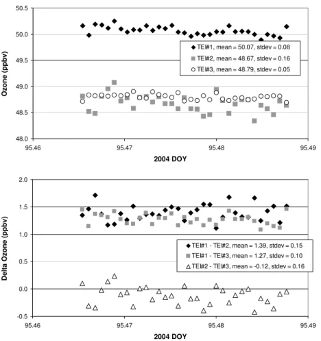
pre-cision. Figure 3 shows a time series from a 30-min inter-comparison measurement,

20

when all inlets were kept at the same height. The upper graph shows the ozone am-bient air mixing ratio recorded with each monitor. The lower graph shows the 1-min

diff_{erence in the measurement between the three possible combinations of instrument}

“gradients”. Since all instruments sampled the same air, the off_{set in the 30-min mean}

value (data shown in the lower graph) represents the instrument bias in the gradient

25

measurement. The off_{set values from the twice daily inter-comparison experiments}

(14)

AMTD

4, 1021–1059, 2011

for measurement

F. Bocquet et al.

◭ ◮

Discussion

P

a

per

|

Dis

cussion

P

a

per

|

Discussion

P

a

per

|

Discussio

n

P

a

per

|

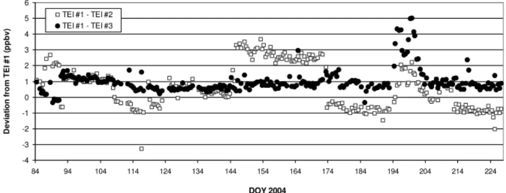
from this series of twice-daily inter-comparison data points. This running mean cor-rection function was then used to calculate, at 1-min resolution, corcor-rection factors that were applied to the entire 1-min ozone gradient data series. The data record in Fig. 4

show that during most times, the determined off_{set between instruments was relatively}

stable, with changes in the relative instrument off_{sets between analyzers of 0.1–0.2}

5

ppbv between inter-comparisons. Notably, the TEI #1 versus TEI #3 comparison pro-duced a more consistent data record then TEI #1 minus TEI #2. It is also obvious that there were several occasions when one of the analyzers experienced a 2–3 ppbv sensitivity jump. Those sensitivity changes in some cases occurred very suddenly, but in other cases happened over the course of 1–2 days. We were not able to identify any

10

obvious causes for these sensitivity changes.

The tower gradient measurements of meteorological variables and ozone were fil-tered according to various instrumental and environmental criteria. Meteorological data were filtered for instruments threshold (for the cup anemometer data), wind

di-rection, and rime buildup on the sensors. Data from the 320◦ to 35◦N sector were

15

eliminated due to tower shadowing and air flow from the camp. Ozone data were examined for miscellaneous artifacts such as low flow in one of the ozone moni-tors and low monitor temperature when the instrument container was open for in-strument maintenance. Data processing also included filtering for atmospheric sta-bility (₋0.1<Ri<0.1), boundary layer height (PBL had to be greater than 100 m for

20

{10–2 m} fluxes and greater than 20 m for {2–0.75 m} fluxes), and friction velocity

(0.05<u∗<0.5 m s−1), where u∗was calculated according to

u∗=_k ∆u

lnz2

z₁

(ΦM)

−1

. (8)

where k is again the van Karman constant. As mentioned above, the gradient flux

measurement method holds for near-neutral atmospheric conditions. The applicability

25

(15)

AMTD

4, 1021–1059, 2011

for measurement

F. Bocquet et al.

◭ ◮

Discussion

P

a

per

|

Dis

cussion

P

a

per

|

Discussion

P

a

per

|

Discussio

n

P

a

per

|

∼2 m on the tower from June to the end of the study period) with calculations of these

same variables from the gradient measurements. For this purpose, the atmospheric

stability parameterz

L, wherez is the distance from the ground andL is the

Monin-Obukhov length, was calculated from the turbulence measurements, and converted

to the Richardson number (Ri, derived from the gradient measurements) according

5

to the relationships given by Kaimal and Finnigan (1994). The comparison showed

that the best agreement (correlation with R2_∼0.65) was obtained for Ri numbers of

−0.10<Ri<+_{0.10. Approximately 95% of the flux data fell within this range. Data}

outside of this range of Ri values were discarded as it appeared that the gradient

method would overestimate fluxes owing to an overestimation of the stability function

10

correction (Cohen, 2006; Cohen et al., 2007).

Another requirement for the flux gradient method is that measurements have to be conducted within the atmospheric surface layer (also known as the constant flux layer), which is defined as the lowest 10% of the mixed boundary layer. Since direct mixed

boundary layer height measurements were not available the boundary layer heightH

15

was estimated using the equation given by Pollard et al. (1973):

H=₁_.₂_u_·₍_{f N}₎−0.5 ₍₉₎

wheref is the Coriolis force (s−1) andN is the Br ünt-V äis äl ä frequency (s−1). Neff_et

al. (2007) reported that this simple equation gave good results compared to other tech-niques, such as minisodar and tethered balloon for measurements over snow. Cohen

20

et al. (2007) recently used the equation to calculate boundary layer heights at Summit and reported that boundary layer heights are lowest during the night and reached their peaks during daytime, with heights of 250–400 m. A filter was then applied

eliminat-ing data whenH was below 100 m, respectively 20 m for the{10–2 m}and{2–0.75 m}

gradient measurements.

25

(16)

AMTD

4, 1021–1059, 2011

for measurement

F. Bocquet et al.

◭ ◮

Discussion

P

a

per

|

Dis

cussion

P

a

per

|

Discussion

P

a

per

|

Discussio

n

P

a

per

|

very high wind conditions, where gradients became too small to be identified by our

measurements. This filter was based on calculations of the friction velocity, u∗. Data

were excluded when friction velocity was lower than a critical value of 0.05 m s−1 or

higher than 0.5 m s−1.

Applying all the above mentioned filters removed a total of _∼57% of data from the

5

entire (6500) 30-min flux gradient data averages (Bocquet, 2007). Table 1 provides the details of how much data were removed by each of the filter criteria for the spring (here defined as day of year (DOY) 92–152) and summer period (DOY 153–227). This data rejection created data gaps of various lengths ranging from 1 point, i.e. 30 min, to

about 30 data points, i.e.,_∼half a day). These gaps can potentially bias analyses from

10

subsequent calculations and interpretations of fluxes (e.g., Goulden et al., 1996; Oren et al., 2006; Dragoni et al., 2007). As gap filling increases uncertainty of calculated fluxes (Falge et al., 2001a, b) we did not pursue this approach.

5 Monte carlo simulations

The relative contribution of individual input variables to the uncertainty of the flux

deter-15

mination was assessed by Monte Carlo simulation. The uncertainty was calculated for

the 30-min average ozone exchange measurement results obtained for the_{2–0.75 m_}

and{10–2 m}gradient measurements. Thirty-min averages and estimated

uncertain-ties were used for the input variables of air temperature gradient, wind speed gradient, ozone mixing ratio gradient, and ambient pressure, and measurement height

gradi-20

ent. Measurement uncertainty estimates were derived from the ensemble of inter-comparison experiments and from estimates of sensor accuracy and measurement precision. Utilized uncertainty values (see further discussion below) were 5 cm for the

measurement height, 0.05 m s−1for the wind speed measurement, 0.05◦C for the

tem-perature measurement, 0.5 hPa for the pressure measurement, and 0.1 ppbv for the

25

(17)

AMTD

4, 1021–1059, 2011

for measurement

F. Bocquet et al.

◭ ◮

Discussion

P

a

per

|

Dis

cussion

P

a

per

|

Discussion

P

a

per

|

Discussio

n

P

a

per

|

ozone exchange velocity. The Monte Carlo sensitivity analysis also investigated how the distribution of the output variable (ve(O3)) varied with changes in only one input variable (while all other input variables are held constant at their 30-min value). This analysis, called the nominal-range analysis, was used to determine which input vari-able(s) had the largest influence on the output uncertainty.

5

6 Results and discussion

6.1 Characterization of measurement precision/accuracy

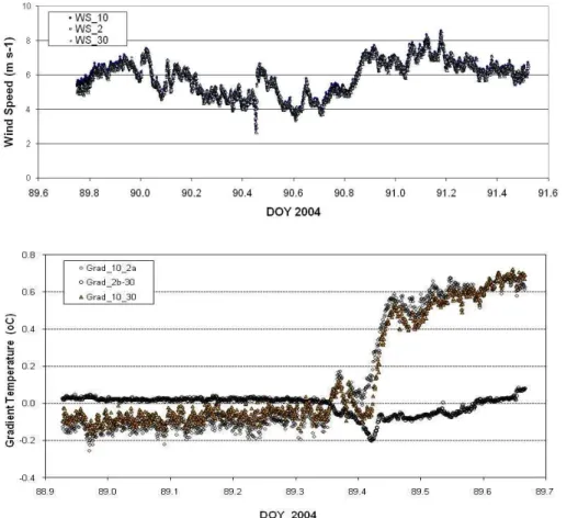
Sensors calculating wind speed and temperature gradients were inter-compared at the beginning, mid-term, and at the tend of the campaign by moving the instruments to the same height for 1–2 days. The insert in Fig. 1 depicts the arrangement for the

10

wind speed sensor inter-comparison. The data obtained from these periods were care-fully evaluated and polynomial-fit correction functions were determined by which two of the sensors were corrected to the third one. Figure 5 presents an example of the raw inter-comparison data for the wind speed and the temperature gradient measurements. The wind speed measurements showed a high level of agreement. Deviations in the

15

uncorrected data between the three wind speed sensors were generally<0.2 m s−1.

After applying the correction functions the deviation between the three sensors was

<0.05 m s−1. Similar results have been obtained for these instruments in two other subsequent field campaigns. Deviations in the temperature measurements were more variable, depending on the particular sensor pair and time of day. A particular diffi_culty

20

stemmed from variable response of the three sensors during high solar irradiance con-ditions. This eff_{ect was identified during the temperature inter-calibration experiments,}

and most pronounced during sunny, mid-day summer conditions. From the data exam-ple in Fig. 5, it is obvious that while there was good agreement during the nighttime and morning hours, the temperature measurement from the 10 m-instrument was

bi-25

(18)

AMTD

4, 1021–1059, 2011

for measurement

F. Bocquet et al.

◭ ◮

Discussion

P

a

per

|

Dis

cussion

P

a

per

|

Discussion

P

a

per

|

Discussio

n

P

a

per

|

is obvious that the measurement from the 10 m instrument was noisier than for the

two other sensors. This eff_{ect has been related to the high albedo of the snow}

sur-face, exposing the downwards pointing aspirator inlets to variable and at times high levels of upwards dwelling irradiance depending on time of day and solar zenith angle. Further discussion and approaches for correction are discussed by Cohen (2006).

Co-5

hen’s study also presented a comparison between results for the heat flux calculations from the tower gradient measurements with directly measured eddy covariance heat flux results. While both data sets agreed well during night and twilight hours, gradient heat flux results during noon hours were up to three times larger than eddy covariance results. These findings motivated Cohen to determine ozone surface fluxes by the

10

“modified gradient” technique, where fluxes were determined using the ozone gradient, and the sonic anemometer turbulence measurements.

The temperature sensor inter-comparisons showed that overall, disagreement in the

uncorrected temperature gradient data was up to 0.6◦C, with the lower gradient pair

typically yielding a lower error than for the tower upper gradient temperature. Data

15

from the inter-comparison periods were subjected to a correction algorithm that had a dependency on solar irradiance. This same algorithm was then also applied to the subsequent inter-comparison (conducted 1–2 months later), and residual errors be-tween these measurements were then estimated from the deviation of the data during this comparison. For the Summit 2004 experiment, we estimate the accuracy of the

20

temperature gradient measurement, after applying the correction functions, to be 0.05–

0.1◦C for the lower gradient interval, and 0.2◦C for gradients that include

measure-ments from the 10 m tower height. In a subsequent experiment at Summit, using new

thermocouple wires with the same instruments, and a slightly diff_{erent intercomparison}

procedure, similar eff_{ects were observed during high solar irradiance conditions. For}

25

that experiment the residual accuracy error of the temperature gradient determination

was estimated to be 0.10–0.15◦C. Please note that a 50% reduced variability during

high irradiance conditions has since been achieved with a diff_{erent aspirated}

(19)

AMTD

4, 1021–1059, 2011

for measurement

F. Bocquet et al.

◭ ◮

Discussion

P

a

per

|

Dis

cussion

P

a

per

|

Discussion

P

a

per

|

Discussio

n

P

a

per

|

Company, Traverse City, MI), using a platinum RTD sensor instead of thermocouple wires.

In summary, for the 2004 experimental conditions, the estimated residual accuracy errors in the wind speed and temperature gradient determinations were on the order of 0.05 m s−1and 0.1◦C. Both of these measurements show a relatively low level of noise.

5

Furthermore, since fluxes are calculated from thirty 1-min data points, the precision

error is reduced by a factor of 1/√30. Consequently, the precision error of the wind

speed and temperature measurement is relatively small in relation to the accuracy error, resulting in the overall uncertainty in the 30-min data to be primarily determined by the accuracy of the measurement. Therefore, the uncertainty estimate was based

10

on the estimation of the accuracy error of this determination.

Precision and accuracy of the ozone measurements were estimated from the twice-daily inter-comparisons. Over the 30-min inter-comparisons period, the standard devi-ation calculated for for the 1-min data reflects both the precision of the measurements (σ) and the change of ambient ozone in time (∆_O_3,amb_/∆_t_):

15

dO3

d t =σ+

∆_O_3,amb

∆_t (10)

When the change of ambient ozone in time (∆_O_3,amb_/∆_t_{) over 30-min becomes small}

(i.e. during conditions when ambient air ozone concentrations do not change), this measurement allows to estimate an approximate value of the precision of the ambient ozone measurement of each monitor. Secondly, the inter-comparison measurements

20

allow determining the off_{set for the ozone gradient measurement, as well as the}

accu-racy and precision of the gradient determination. The inter-comparison example shown in Fig. 3 reflects a case with relatively stable ozone concentrations. The deviations between the 1-min ozone readings mostly reflect the precision of the ozone measure-ment for each analyzer. For this particular example, the variability/precision over the

25

30-min measurement period was 0.08, 0.16, and 0.05 ppbv for monitors #1, 2, and 3, respectively. Obviously, there is a factor of approximately 3 diff_{erence in the achieved}

(20)

AMTD

4, 1021–1059, 2011

for measurement

F. Bocquet et al.

◭ ◮

Discussion

P

a

per

|

Dis

cussion

P

a

per

|

Discussion

P

a

per

|

Discussio

n

P

a

per

|

configuration and history, there was no obvious reason for this diff_{erence in}

perfor-mance. A histogram of the results from all_∼300 inter-comparisons showed that the

TEI monitors under these deployment conditions yielded a best case 1-min measure-ment precision on the order of 0.05–0.08 ppbv during the 30-min periods. From that, using error propagation rules, one would theoretically expect a precision of the gradient

5

measurement of 0.07–0.11 ppbv. This estimate agrees well with the calculation of the “gradient” measurements during the inter-comparison periods. The average precision for the three ozone diff_{erentials from all experiments was 0.098/0.085/0.11 ppbv for the}

three instrument pairs. Since precision errors are additive in the ozone gradient deter-mination, the error for the 30-min mean values, derived from the 1-min gradients data

10

are estimated to account to (divided by√30) 0.02–0.03 ppbv. Consequently, similarly

as for the wind speed and temperature measurement, the uncertainty in the ozone measurement is primarily due to the accuracy of the ozone measurement, which in turn, is mostly determined by the sensitivity drift of each individual analyzer over time. From the extensive testing and inter-comparisons of the three TEI, we estimated the

15

overall uncertainty in the corrected ozone gradient determination to be_∼0.1 ppbv.

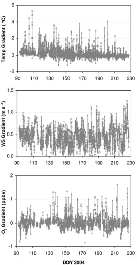
6.2 Gradient data

The gradient results for temperature, wind speed, and ozone for the entire campaign

for the {2–0.75 m} gradient height are shown in Fig. 6. These data reflect the tower

gradients that were determined after application of all corrections and filters as

dis-20

cussed above. Most temperature gradients were in the 0–1◦C range, with occasional

values approaching 3–5◦C. Those higher values resulted from stable stratification

dur-ing nighttime conditions, when strong inversion layers over the cold snow surface were encountered. These conditions typically fell outside of the stability range considered

for flux calculations. Negative gradients, on the order of 0 to−1◦C, occurred during

25

(21)

AMTD

4, 1021–1059, 2011

for measurement

F. Bocquet et al.

◭ ◮

Discussion

P

a

per

|

Dis

cussion

P

a

per

|

Discussion

P

a

per

|

Discussio

n

P

a

per

|

2-m height were always higher than at 0.75 m, causing wind speed gradients to always be positive. There was a large variability in wind speed gradients, ranging from<0.1 to

∼1.2 ms−1. Ozone gradients between the lower two tower inlets exceeded±1 ppbv on

occasions, but most gradients were in the order of tenths of ppbv or smaller.

6.3 Uncertainty estimation

5

An uncertainty estimate in the ozone flux (deposition velocity) determination was de-rived from the Monte Carlo simulation for each 30-min flux average interval. Figure 7 shows two examples of 30-min deposition velocity results for a spring and summer day,

with the 1-σ and 2-σ uncertainty estimate margins added to the data. These

simula-tions yielded an estimated uncertainty (1σ) in the ozone exchange velocity result from

10

0.005 to 0.038 cm s−1) in this particular example. The review of all simulations yields a medium uncertainty on the order of 10−2cm s−1in general. It is obvious that the un-certainty in the data has a significant magnitude in relation to the overall size of the signal (high relative error). Another notable observation is that the absolute value of the uncertainty increases with the size of the signal. Besides providing the uncertainty

15

estimate of each individual flux result, this calculation also allowed evaluating the rela-tive contribution of the measured variables towards the overall ozone flux uncertainty. The review of these results showed that there is a high variability in the relative con-tribution of individual measurements to the uncertainty in the flux result. This stems from the fact that gradient results, depending on encountered conditions, are highly

20

variable. Typically, gradients for temperature and ozone increase with increasing at-mospheric stability, conditions that at Summit are more prominent earlier in the year, and during nighttime. When gradients are large, the relative uncertainty in the gradient measurement (and flux determination) becomes smaller. Vice versa, moving towards neutral and unstable conditions, as gradients become smaller, the relative uncertainty

25

(22)

AMTD

4, 1021–1059, 2011

for measurement

F. Bocquet et al.

◭ ◮

Discussion

P

a

per

|

Dis

cussion

P

a

per

|

Discussion

P

a

per

|

Discussio

n

P

a

per

|

review of the 300+_{Monte Carlo outputs showed that the ozone measurement typically}

has the highest contribution to the overall variability in the outputs, contributing on the order of 50–90% to the variance. The second highest contribution was from the wind speed measurement, followed by the temperature measurement, the height determi-nation, and pressure. The relatively low ranking and contribution of the temperature

5

variable was somewhat surprising. Particularly during unstable conditions, tempera-ture gradients in the surface layer become small, turning the measurement uncertainty in the gradient measurement into a relative large error. There is an obvious explanation for the robustness of the flux determination towards the uncertainty in the temperature measurement. In the flux calculation, the temperature gradient is factored in through

10

the computation ofRi and the stability function. Those correction factors become

in-creasingly important with increasing departure from neutral stability conditions. Since data were previously rigorously filtered for atmospheric stability, the remaining data set reflects mostly near-neutral conditions, where stability functions calculated with the temperature data have a lower influence on the flux calculation.

15

6.4 Ozone deposition results

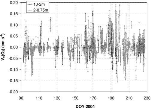
Ozone v_e results from the entire 2004 campaign are shown in Fig. 8. Gaps in the

data plot are, as discussed above, mostly due to exclusion of measurement periods

from the data filtering. Determined ozoneve values show a significant variability, but

generally fall within the range of₋0.05 to+_{0.15 cm s}−1_{. There is a tendency towards}

20

larger ozone deposition fluxes, and more distinct diurnal cycles towards the summer months. This behavior is most apparent in the averaged (1 week) diurnal cycles shown

for one spring and one late summer week in Fig. 9. During spring, ozonevefall within

the narrow range of 0.00+_/₋_{0.01 cm s}−1_{. During summertime, nighttime minima and}

afternoon maxima are up to 10–15 times larger. Results from these flux gradient

deter-25

(23)

AMTD

4, 1021–1059, 2011

for measurement

F. Bocquet et al.

◭ ◮

Discussion

P

a

per

|

Dis

cussion

P

a

per

|

Discussion

P

a

per

|

Discussio

n

P

a

per

|

from this same summer data set, as well as from a later springtime experiment. The dependency of the ozone flux on wind speed and solar irradiance, both during spring and during summer, is shown in Fig. 10. During summer, there is an obvious ten-dency of larger ozone deposition fluxes at times of high solar irradiance, and during high winds. This behavior can be explained by apparent ozone destruction seen inside

5

the snowpack and wind pumping eff_{ects, causing faster exchange of snowpack}

inter-stitial air with the atmosphere above the snow during high winds. The data shown in Fig. 9 and Helmig et al. (2009) illustrate that during certain times there appears to be an upward flux of ozone from the snow surface. This behavior suggests ozone produc-tion near the snow surface. Elucidaproduc-tion of the underlying chemical processes driving

10

this phenomenon is the context of new research that builds upon the findings from the studies presented here.

6.5 Evaluation of the ozone flux method

The measurement uncertainty of approximately 0.01 cm s−1 for the ozone exchange

velocity allowed deciphering the general seasonal behavior of the ozone flux

behav-15

ior at Summit, as well as diurnal changes during the summer. However, the achieved sensitivity was not suffi_{cient for resolving fine scale flux behavior during the winter}

pe-riod. There are few other studies that have accomplished ozone flux measurements at this sensitivity, respectively that have provided characterization of their achieved flux measurement sensitivity. We are not aware of any research that has reported

20

higher sensitivity (respectively lower uncertainty) in ozone flux determination. Recently, Bariteau et al. (2009) described an eddy covariance method for ozone flux measure-ments from a ship-borne platform for the study of ozone update to the ocean. Similarly to snow, ozone update rates to water are low, with deposition velocities on the order

of 0.01–0.05 cm s−1. This eddy covariance system achieved a similar resolution as our

25

(24)

AMTD

4, 1021–1059, 2011

for measurement

F. Bocquet et al.

◭ ◮

Discussion

P

a

per

|

Dis

cussion

P

a

per

|

Discussion

P

a

per

|

Discussio

n

P

a

per

|

7 Summary and conclusions

These experiments define a protocol for ozone flux measurements by the

aerody-namic gradient method using off_{-the-shelf meteorological and chemical sensors.}

Inter-comparison measurements that were conducted by bringing meteorological and chem-ical sensors (inlet height) to the same height were found to be an essential step for

5

minimizing the uncertainty in the gradient determination and flux calculation. This find-ing is in agreement to the previous study reported by Dragoni et al. (2007). Usfind-ing our

protocol, the uncertainty in the ozone measurement was reduced to_∼0.1 ppbv for

30-min averaged ozone gradient data. These measurements allowed deciphering ozone exchange velocities on the order of_∼10−2cm s−1in magnitude. This is one of the most

10

sensitive ozone flux determinations reported in the literature to date. Monte Carlo sim-ulations showed an uncertainty of the 30-min ozone exchange velocity on the order

of magnitude of 10−2cm s−1. The Monte Carlo sensitivity analysis revealed that the

gradient measurements of the ozone mixing ratio is the variable having the highest contribution towards the uncertainty in the ozone flux measurement, followed by the

15

wind speed gradient and temperature gradient measurement.

Measurements conducted at Summit resulted in ozone ve values on the order of

0.01+_/₋_{0.01 cm s}−1 _{during springtime, and between} ₋_{0.03 to 0.15 cm s}−1_{during the}

summer. During summer, ozone fluxes showed a distinct diurnal cycle, with increased ozone deposition rates occurring during mid-afternoon hours. Results also showed

20

increase of ozoneve with increasing winds, an effect that can be explained by faster

exchange of ozone depleted air in the snowpack from wind pumping. These findings provide new constraints for the representation of ozone deposition to snow in polar

regions. As our ozone ve from Summit in general are smaller than the previously

reported data from mid-latitudes, and smaller than ozoneve currently considered in

25

(25)

AMTD

4, 1021–1059, 2011

for measurement

F. Bocquet et al.

◭ ◮

Discussion

P

a

per

|

Dis

cussion

P

a

per

|

Discussion

P

a

per

|

Discussio

n

P

a

per

|

Supplementary material related to this article is available online at: http://www.atmos-meas-tech-discuss.net/4/1021/2011/

amtd-4-1021-2011-supplement.pdf.

Acknowledgements. This research has been supported through the United States National Science Foundation (Office of Polar Programs OPP #240976). We thank Thermo Fisher Scien-5

tific for modifying the TEI 49C ozone monitor data acquisition program. Logistical support was provided by VECO Polar Resources and the US 109thAir National Guard. We also thank the Danish Commission for Scientific Research for providing access to the Summit research site.

References

Albert, M. R. and Hawley, R. L.: Seasonal differences in surface energy exchange and accu-10

mulation at Summit, Greenland. Ann. Glac., 31, 387–390, 2000.

Aldaz, L.: Flux measurements of atmospheric ozone over land and water, J. Geophys. Res., 74, 6934–6946, 1969.

Bariteau, L., Helmig, D., Fairall, C. W., Hare, J. E., Hueber, J., and Lang, E. K.: Determination of oceanic ozone deposition by ship-borne eddy covariance flux measurements, Atmos. Meas. 15

Tech., 3, 441–455, doi:10.5194/amt-3-441-2010, 2010.

Bocquet, F.: Surface layer ozone dynamics and air-snow interactions at Summit, Greenland: spring and summer ozone exchange velocity and snowpack ozone-the complex interactions, Unpublished PhD thesis, University of Colorado, Boulder, 247 pp., 2007.

Brook, R. R.: The influence of water vapor fluctuations on turbulent fluxes, Bound.-Lay Meteo-20

rol., 15, 481–487, 1978.

Cohen, L.: Boundary layer characteristics and ozone fluxes at Summit, Greenland, M.S. Thesis, University of Colorado, 2006.

Cohen, L., Helmig, D., Neff_{, W., Grachev, A., and Fairall, C.: Boundary-layer dynamics and its} influence on atmospheric chemistry at Summit, Greenland, Atmos. Environ., 41, 5044–5060, 25

(26)

AMTD

4, 1021–1059, 2011

for measurement

F. Bocquet et al.

◭ ◮

Discussion

P

a

per

|

Dis

cussion

P

a

per

|

Discussion

P

a

per

|

Discussio

n

P

a

per

|

Colbeck, I. and Harrison, R. H.: Dry deposition of ozone: some measurements of deposition velocity and of vertical profiles to 100 meters, Atmos. Environ., 19, 1807–1818, 1985. Cullen, N. J.: Characteristics of the atmospheric boundary layer at Summit, Greenland,

Unpub-lished PhD thesis, University of Colorado at Boulder, 2003.

Dabberdt, W. F., Lenschow, D. H., Horst, T. W., Zimmerman, P. R., Oncley, S. P., and Delany, A. 5

C.: Atmosphere-surface exchange measurements, Science, 260, 1472–1481, 1993.

Dragoni, D., Schmid, H. P., Grimmond, C. S. B., and Loescher, H. W.: Uncertainty of annual net ecosystem productivity estimated using eddy covariance flux measurements, J. Geophys. Res., 112, D17102, doi:10.1029/2006JD008149, 2007.

Falge, E., Baldocchi, D., Olson, R.J., Anthoni, P., Aubinet, M., Bernhofer, C., Burba, G., Ceule-10

mans, R., Clement, R., Dolman, H., Granier, A., Gross, P., Grunwald, T., Hollinger D., Jensen N.-O., Katul, G., Keronen P., Kowalski, A., Chun, T.L., Law, B., Meyers, T., Moncrieff_{, J.,} Moors, E., Munger, W., Pilegaard, K., Rannik, ¨U., Rebmann, C., Suyker, A., Tenhunen, J., Tu, K., Verma, S., Vesala, T., Wilson, K., and Wofsy, S.: Gap filling strategies for defensible annual sums of net ecosystem exchange, Agric. Forest Meteorol., 107, 43–69, 2001a. 15

Falge, E., Baldocchi, D., Olson, R.J., Anthoni, P., Aubinet, M., Bernhofer, C., Burba, G., Ceule-mans, R., Clement, R., Dolman, H., Granier, A., Gross, P., Grunwald, T., Hollinger D., Jensen N.-O., Katul, G., Keronen P., Kowalski, A., Chun, T.L., Law, B., Meyers, T., Moncrieff, J., Moors, E., Munger, W., Pilegaard, K., Rannik, ¨U., Rebmann, C., Suyker, A., Tenhunen, J., Tu, K., Verma, S., Vesala, T., Wilson, K., and Wofsy, S.: Gap filling strategies for long-term 20

energy flux data sets, a short communication, Agric. Forest Meteorol., 107, 71–177, 2001b. Galbally, I.: Some measurements of ozone variation and destruction in the atmospheric surface

layer, Ibid., 218, 456–457, 1968.

Galbally, I. and Allison, I.: Ozone fluxes over snow surfaces, J. Geophys. Res., 77, 3946–3949, 1972.

25

Ganzeveld, L. and Lelieveld, J.: Dry deposition parameterization in a chemistry general circu-lation model and its influence on the distribution of reactive gases, J. Geophys. Res., 100, 20999–21012, 1995.

Goulden, M. L., Munger, J. M., Fan, S.-M., Daube, B. C., and Wofsy, S. C.: Measurements of carbon sequestration by long-term eddy covariance: methods and a critical evaluation of 30

accuracy, Glob. Change Biol., 2, 169–182, 1996.