www.atmos-meas-tech.net/3/853/2010/ doi:10.5194/amt-3-853-2010
© Author(s) 2010. CC Attribution 3.0 License.
Measurement
Techniques
Lag time determination in DEC measurements with PTR-MS
R. Taipale1, T. M. Ruuskanen1,2, and J. Rinne1
1University of Helsinki, Department of Physics, P.O. Box 64, 00014 University of Helsinki, Finland
2University of Innsbruck, Institute of Ion Physics and Applied Physics, Technikerstr. 25, 6020 Innsbruck, Austria Received: 8 December 2009 – Published in Atmos. Meas. Tech. Discuss.: 8 February 2010
Revised: 15 June 2010 – Accepted: 30 June 2010 – Published: 7 July 2010
Abstract. The disjunct eddy covariance (DEC) method has emerged as a popular technique for micrometeorological flux measurements of volatile organic compounds (VOCs). It has usually been combined with proton transfer reaction mass spectrometry (PTR-MS), an online technique for VOC con-centration measurements. However, the determination of the lag time between wind and concentration measurements has remained an important challenge. To address this issue, we studied the effect of different lag time methods on DEC fluxes. The analysis was based on both actual DEC measure-ments with PTR-MS and simulated DEC data derived from high frequency H2O measurements with an infrared gas ana-lyzer. Conventional eddy covariance fluxes of H2O served as a reference in the DEC simulation. The individual flux mea-surements with PTR-MS were rather sensitive to the lag time methods, but typically this effect averaged out when the me-dian fluxes were considered. The DEC simulation revealed that the maximum covariance method was prone to overes-timation of the absolute values of fluxes. The constant lag time methods, one based on a value calculated from the sam-pling flow and the samsam-pling line dimensions and the other on a typical daytime value, had a tendency to underestimate. The visual assessment method and our new averaging ap-proach utilizing running averaged covariance functions did not yield statistically significant errors and thus fared better than the habitual choice, the maximum covariance method. Given this feature and the potential for automatic flux calcu-lation, we recommend using the averaging approach in DEC measurements with PTR-MS. It also seems well suited to conventional eddy covariance applications when measuring fluxes near the detection limit.
Correspondence to:R. Taipale ([email protected])
1 Introduction
Volatile organic compounds (VOCs) affect tropospheric chemistry mainly through their reactions with OH, NO3, and O3(e.g. Koppmann, 2007). Some of them are deemed major contributors or inhibitors to aerosol particle formation and growth (e.g. Hoffmann et al., 1997; Claeys et al., 2004; Hal-lquist et al., 2009; Kiendler-Scharr et al., 2009), thus making VOC measurements essential for the current climate change research. Globally, natural VOC emissions (about 1150 Tg (C) per year) are estimated approximately ten times higher than emissions due to human activity (Guenther et al., 1995). Micrometeorological flux measurements with the eddy co-variance method have yielded fundamental information on ecosystem scale VOC emissions (e.g. Guenther and Hills, 1998; Shaw et al., 1998; Karl et al., 2001, 2002; Warneke et al., 2002; Spirig et al., 2005; Brunner et al., 2007; Rinne et al., 2007). Many of these measurements have relied on an approach called disjunct eddy covariance (DEC; Rinne et al., 2001; Karl et al., 2002), which has usually been combined with proton transfer reaction mass spectrometry (PTR-MS), an online technique for measuring VOC concentrations (e.g. Lindinger et al., 1998; de Gouw and Warneke, 2007; Blake et al., 2009). In addition to theoretical considerations and data simulations (e.g. Kaimal and Gaynor, 1983; Lenschow et al., 1994), field studies have shown that DEC is a reliable and robust method for trace gas flux measurements (Rinne et al., 2008; Turnipseed et al., 2009; H¨ortnagl et al., 2010).
response times of less than 0.5 s, the present PTR-MS instru-ments are adequate for multi-compound DEC measureinstru-ments with continuous sampling flow, sometimes referred as vir-tual DEC (Karl et al., 2002). Slower instruments require an additional intermediate sample container for disjunct sam-pling (Rinne et al., 2001), or alternatively, high frequency corrections in the post-processing of flux data (Davison et al., 2009).
When measuring gas or particle fluxes, a major pragmatic challenge in EC and DEC is to determine the lag time be-tween wind and concentration measurements, i.e., the delay caused by the sample transit time through the sampling line. Once the lag time has been determined, the time series can be synchronized, and the flux value is given by the covariance derived from the matched time series. A straightforward lag time calculation based on the sampling flow and the sam-pling line dimensions is an inadvisable option as the flow often varies, at least during an extended measurement period (e.g. Shimizu, 2007). Further, the lag time appears to de-pend on the compound, an unpleasant feature for VOC flux measurements. This is suggested by the compound-specific attenuation of turbulent fluctuations in the sampling line (e.g. Su et al., 2004).
The prevalent solution is to calculate the covariance as a function of lag time, and then determine the maximum ab-solute value of the covariance within a reasonable lag time window (e.g. McMillen, 1988; Aubinet et al., 2000). This method can be automated reliably if the maximum is dis-tinct, like in most EC measurements of CO2 and H2O for instance. However, noisy covariance functions, common in DEC measurements, require usually visual judgement (Rinne et al., 2007; Davison et al., 2009). Such manual assessment is somewhat dependent on the person, prone to human errors, and burdensome, but it may be the only viable option when measuring small VOC fluxes. Still, an automated and objec-tive regime would systematize and hasten data processing.
In addition to the challenging lag time determination, noisy covariance functions inflict other difficulties on flux calculation. When the lag time is derived from the maxi-mum absolute covariance, a systematic overestimation of the absolute flux is possible. Of course, this flaw also afflicts EC measurements relying on such lag time method, but its im-pact is even more harmful in DEC where the signal-to-noise ratio tends to be lower.
This paper addresses the lag time problem, a timely conun-drum for many research groups as the combination of DEC and PTR-MS has emerged as a popular tool in VOC flux measurements. We present an explicit comparison of five lag time methods and illustrate how they affect fluxes mea-sured with DEC. We consider two variants of the constant lag time approach. Both of them are based on preset values, one calculated from the sampling flow and the sampling line di-mensions, the other representing a typical daytime value de-duced from measurements with distinct covariance function maxima. We also evaluate the maximum covariance method,
which is the habitual choice in EC, our new averaging ap-proach, and the visual assessment method. The averaging approach strives to facilitate automated lag time determina-tion by reducing the noise in a covariance funcdetermina-tion. Although our new method is mainly intended for DEC measurements with PTR-MS, it might be useful for any application affected by noisy covariance functions, i.e., when measuring fluxes near the detection limit. One current application could be EC measurements with the novel PTR-MS instrument equipped with a time-of-flight mass analyzer (e.g. Blake et al., 2009; M¨uller et al., 2010).
To assess the performance of different lag time methods, we first look at high frequency H2O measurements by an in-frared gas analyzer. In the absence of a direct reference for our DEC measurements, we simulate them by adding noise to the original H2O data and then converting it into a dis-junct time series. This manipulated H2O signal is thought to resemble a typical VOC measurement by PTR-MS. EC mea-surements of H2O fluxes are regarded as a reference for this DEC simulation.
Next, we probe how the lag time methods affect actual DEC fluxes measured by PTR-MS. Given the good correla-tion between the PTR-MS water cluster ion signal, detected at 37 amu (M37), and the ambient H2O concentration (Am-mann et al., 2006), contrasting M37 fluxes with the refer-ence H2O fluxes can shed light on the lag time problem. Fi-nally, we illustrate the influence of lag time determination on fluxes of two classic subjects in PTR-MS studies, methanol and monoterpenes.
2 Methods
2.1 Measurements
The SMEAR II (Station for Measuring Ecosystem– Atmosphere Relations II) station of the University of Helsinki served as the measurement site (for a review, see Hari and Kulmala, 2005). It was situated at a rather homo-geneous 45-year-old Scots pine (Pinus sylvestris) dominated forest in southern Finland (61◦51′N, 24◦17′E, 180 m a.s.l.). The measurements were performed in 9–14 August 2007.
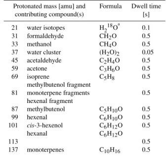
Table 1. PTR-MS measurement cycle in the DEC measurements, the compounds contributing to the measured masses, and the PTR-MS integration times. The cycle length was 6.6 s.
Protonated mass [amu] and Formula Dwell time
contributing compound(s) [s]
21 water isotopes H218Oa 0.1
31 formaldehyde CH2O 0.5
33 methanol CH4O 0.5
37 water cluster (H2O)2 0.05
45 acetaldehyde C2H4O 0.5
59 acetone C3H6O 0.5
69 isoprene C5H8 0.5
methylbutenol fragment
81 monoterpene fragments 0.5
hexenal fragment
87 methylbutenol C5H10O 0.5
99 hexenal C6H10O 0.5
101 cis-3-hexenol C6H12O 0.5
hexanal C6H12O
113 0.5
137 monoterpenes C10H16 0.5
athe most abundant isotope
The PTR-MS measurement cycle lasted 6.6 s and contained 13 masses which were measured successively (Table 1). The sampling time was 0.5 s for each VOC-related mass, 0.1 s for the primary ion isotopes, and 0.05 s for the water cluster ions. Also the vertical wind speed was recorded in the PTR-MS data to synchronize the clocks of the computers. Only every third hour was allocated for the DEC measurements since the PTR-MS was utilized also in concentration profile and shoot scale emission measurements. Our PTR-MS mea-surement, calibration, and concentration calculation methods have been described in detail by Taipale et al. (2008).
An infrared gas analyzer (IRGA, LI-COR Inc., LI-6262) was used in the H2O measurements. The data were recorded continuously at 10 Hz on the same computer as the wind data of the DEC measurements, which enabled the conventional EC measurements of H2O fluxes. The heated PTFE sam-pling line was 12 m in length and 8 mm in inner diameter. The sampling flow was 13.5 l min−1 for the first 10 m and 12.5 l min−1for the last 2 m. A side flow of 7 l min−1was taken into the IRGA through a PTFE tube, which was 0.5 m in length and 4 mm in inner diameter (for details, see Kero-nen et al., 2003).
2.2 DEC simulation and M37
The DEC simulation was based on the H2O data from the IRGA. To increase noise, normally distributed random num-bers were added to the original time series. The average was not changed whereas the standard deviation was increased by about 13–15%. Figure 1 shows an example of this procedure
0 5 10 15 20 25 30 35 40 45
11.5 12 12.5 13 13.5 14
Time [min]
Concentration [g m
−3
]
H
2Onoise
H
2O
Fig. 1.Example of the original H2O measurements with the IRGA
and the corresponding manipulated signal containing added noise
(9 August 2007 12:00–12:45). The standard deviation of H2Onoise
is 14% higher than that of H2O.
designed to improve the resemblance between the IRGA and PTR-MS measurements. In the later analysis, the manipu-lated H2O signal (H2Onoise) was converted into a disjunct time series using the sampling interval of the actual DEC measurements (6.6 s). The simulation results, the DEC fluxes of H2Onoise, were evaluated against the EC fluxes of H2O.
Although not exclusively dependent on the ambient H2O concentration, the PTR-MS water cluster ion signal (M37) can be employed in H2O flux measurements (Ammann et al., 2006), provided it is routinely calibrated for H2O. Our aim was to study how the different lag time methods affect M37 fluxes and whether some of them yield a better correlation with the reference H2O fluxes. The only treatment for M37 was the conversion into normalized counts per second (ncps) according to the equation proposed by Taipale et al. (2008).
The correlation between the M37 signal and the H2O con-centration varied substantially. When calculated for the 45-min flux averaging time, typical daytime correlation coeffi-cients were 0.65–0.90, but nocturnal values were below 0.30. Hence the EC fluxes of H2O were considered a somewhat rough reference and the motivation focused more on the sen-sitivity of the M37 fluxes to the lag time methods.
2.3 Covariance functions
A covariance function gives the covariance of the vertical wind speed and the gas concentration as a function of lag time (e.g. Kaimal and Finnigan, 1994):
F (1t )= 1
N
N
X
i=1
w′(i−1t /1tw)c′(i). (1)
−200 −150 −100 −50 0 50 100 150 200 −100
0 100 200 300
Lag time [s] H2
O flux [g m
−2
h
−1]
DEC EC
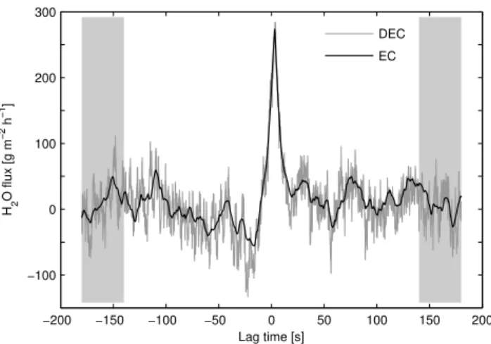
Fig. 2.Covariance function of H2O calculated in the EC and DEC
manner (9 August 2007 12:00–12:45). The comparison illustrates how DEC increases the noise and thus the flux uncertainty. The shaded areas show the lag time ranges used in the uncertainty esti-mation, which was based on the standard deviations of the
covari-ance function. Note that only the EC fluxes of H2O were used as
a reference in the DEC simulation (Sect. 2.2). The DEC version of the covariance function of H2O is a mere illustration.
the VOC or H2O mass concentration or the normalized M37 count rate. The sampling interval in the wind measurements,
1tw, was 0.1 s and the number of measurements during the 45-min flux averaging time,N, was 410 in DEC and 27 000 in EC.
Covariance functions were calculated in the DEC man-ner for methanol (M33), monoterpenes (M137), M37, and H2Onoise, whereas the conventional EC procedure was used for H2O (Fig. 2). In all cases, the lag time window was ±180 s with a time resolution of 0.1 s. Before the calcula-tions, three-dimensional coordinate rotation and linear de-trending were applied to the data using established methods (Kaimal and Finnigan, 1994). As the sampling time was 0.5 s for M33 and M137, five-point running averages of the verti-cal wind speed were used for these masses. The PTR-MS and anemometer data were synchronized time-wise by find-ing the sharp maximum from the autocorrelation function of the vertical wind speed. To make the covariance functions of M33, M37, and M137 temporally concordant, the actual measurement times of these masses within the PTR-MS cy-cle were taken into account.
The flux error estimation was based on the covariance functions. The uncertainty of a flux value was determined by calculating standard deviations from the lag time ranges −180 to −140 s and 140 to 180 s (Wienhold et al., 1994; Spirig et al., 2005). The average of the standard deviations was multiplied by 1.96 to get the 95% confidence interval for each flux measurement (Rinne et al., 2007). Figure 2 il-lustrates the increasing effect of DEC on the flux uncertainty when compared with EC.
0 5 10 15 20 25 30
100 200 300 400
Lag time [s]
M137 flux [
µ
g m
−2
h
−1
]
CALC TYP
MAX AVG
VIS
Original Averaged
Fig. 3.Principles of the lag time methods illustrated with a covari-ance function of M137 (11 August 2007 12:00–12:45). The calcu-lated (CALC) and typical (TYP) constant lag times were 7.1 and 9.9 s. In the maximum covariance method (MAX), the lag time was 10.5 s. The averaging approach (AVG) yielded a lag time of 11.7 s, which was determined from the maximum of the averaged covari-ance function. However, the final flux value was derived from the original covariance function. The visual assessment method (VIS) gave a lag time of 11.0 s.
2.4 Lag time methods
The crux of this study was the comparison of five lag time methods. One of them relied on a theoretical constant value, while in the other methods lag times were determined di-rectly from the covariance functions. As the motivation was stand-alone DEC measurements with PTR-MS, this straight-forward regime was deemed viable. Also more complex and perhaps better alternatives have been proposed (e.g. Shaw et al., 1998; Massman, 2000), but usually they require spec-tral analysis and hence high frequency measurements, which makes them unsuitable for DEC.
The lag time methods were based on the following princi-ples (Fig. 3):
– In the CALC method, the lag time was calculated from the sampling flow and the sampling line dimensions. It was kept constant throughout the measurement period. The values were 2.9 and 7.1 s for the IRGA and PTR-MS measurements, respectively.
09 10 11 12 13 14 15 0
250 500 750 1000 1250 1500
PAR [
µ
mol m
−2 s
−1
]
A
14 16 18 20 22 24 26
Temperature [
oC]
09 10 11 12 13 14 15
0 5 10 15 20
Date (August 2007) H2
Onoise
lag time [s]
B
REF CALC TYP MAX AVG VIS
Fig. 4.(A) Photosynthetically active radiation (PAR), air temperature, and (B) lag time of H2Onoiseas given by the five lag time methods
(Sect. 2.4). The lag time of H2O (REF) was determined with MAX. The EC fluxes of H2O served as a reference in the DEC simulation (see
Fig. 5).
– In the MAX method, the lag time was determined from the maximum absolute value of the covariance function within a given lag time window. This is the prevalent method in EC (e.g. Aubinet et al., 2000). It was applied to the reference EC fluxes of H2O as well as to the DEC fluxes of H2Onoiseusing a lag time window 0–20 s. The window was 0–50 s for M33, M37, and M137.
– In our new averaging approach (AVG), the covariance function was first averaged using a five-second running average to make patterns more distinguishable (Fig. 3). The lag time was derived from this averaged covariance function using the MAX method. Although averaging was practised to aid the lag time identification, the final flux value was always determined from the original co-variance function at the indicated lag time. This ensured that no part of the real flux signal was eliminated due to the averaging. The width of the averaging window was estimated visually using the EC measurements of H2O and the simulated DEC data of H2Onoise. The chosen
window was deemed wide enough to allow a sufficient noise reduction but also narrow enough to prevent a con-siderable shift in the covariance function maximum.
REF CALC TYP MAX AVG VIS 0
100 200 300 400
Flux [g m
−2 h −1]
A
CALC TYP MAX AVG VIS
−120 −90 −60 −30 0 30 60 90
Error [g m
−2 h −1]
B
Fig. 5.DEC simulation results. Panel (A) gives the statistics of the DEC fluxes of H2Onoiseand the EC fluxes of H2O. Panel (B) shows
the error analysis. The DEC fluxes were calculated using the five lag time methods (Sect. 2.4) and evaluated against the reference EC fluxes (REF, Sect. 3.2). The line in the middle of each box is the median. The lower and upper line are the 25th and 75th percentile, the distance between them is the interquartile range. The error bars extend from the top or bottom of the box to the furthest data value within 1.5 times the interquartile range. The values beyond the error bars are outliers. The notches show the 95% confidence interval for the median. If notches of two boxes do not overlap, the difference between medians is statistically significant.
3 Results and discussion
The measurement period 9–14 August 2007 contained a fairly wide range of conditions for micrometeorological flux measurements. The friction velocity peaked typically at 0.5– 0.9 m s−1 in the afternoon and was below 0.25 m s−1 be-tween 21:00 and 06:00. This is a general acceptance thresh-old for flux measurements at the SMEAR II site (Markkanen et al., 2001). The air temperature varied from 15.6 to 25.6◦C and the daily maximum of photosynthetically active radia-tion from 550 to 1330 µmol m−2s−1(Fig. 4a). It was raining only on 12 August.
To enable an explicit comparison of the lag time methods, all measurements were included in the analysis, i.e., no data were filtered out due to the friction velocity threshold or any other quality criterion. A flux measurement was rated unre-liable if the flux uncertainty exceeded the absolute value of the flux. In VIS, the undetermined fluxes were afterwards converted into zeros to allow commensurate median calcula-tions.
3.1 Lag times
A survey of the lag times revealed two important features. Figure 4b illustrates the variation in the lag time of H2Onoise as given by MAX, AVG, and VIS. It also shows the lag time of H2O determined with MAX. In general, the daytime val-ues were smaller and fluctuated remarkably less than the night-time values, although the rainy 12 August did not fit into this pattern. Also M33, M37, and M137 exhibited quite similar behaviour (not shown). The substantial hourly and di-urnal lag time variation indicates that CALC and TYP indeed are inadvisable options. This was somewhat expected as con-stant lag time methods are often considered fundamentally flawed (e.g. Massman, 2000). While typically larger than the constant lag times, the medians determined with MAX, AVG, and VIS never differed significantly at the 95% confidence level. In the case of H2Onoise, they were also in agreement with the median lag time of H2O.
The lag times of M33, M37, and M137 gave more in-sight into VOC flux measurements. Their medians differed slightly despite the same measurement setup and the correc-tion for the actual measurement times within the PTR-MS measurement cycle. The differences were not statistically significant at the 95% confidence level in MAX and AVG, but M33 differed significantly from both M37 and M137 in VIS. The median lag time was 8.1 s for M33, 9.8 s for M37, and 10.5 s for M137. This suggests that the lag time should be de-termined individually for each compound, a result which has also been observed in CO2and H2O studies (e.g. Su et al., 2004; Ibrom et al., 2007).
3.2 DEC simulation results
To assess the performance of the different lag time meth-ods, we resorted to the H2O measurements with the IRGA. Each lag time method was used to determine the DEC fluxes of H2Onoise, the manipulated H2O signal containing added noise (Sect. 2.2). The EC fluxes of H2O served as a refer-ence (REF) for this DEC simulation.
09 10 11 12 13 14 15 0
2000 4000 6000
M37 flux [ncps m s
−1
]
A
CALC: 0.68, 73 ncps m s−1
TYP: 0.79, 85 ncps m s−1
MAX: 0.57, 200 ncps m s−1
AVG: 0.62, 130 ncps m s−1
VIS: 0.76, 96 ncps m s−1
09 10 11 12 13 14 15
−200 0 200 400 600
M33 flux [
µ
g m
−2
h
−1
]
B CALC: 17
µg m−2 h−1 TYP: 18 µg m−2 h−1
MAX: 41 µg m−2 h−1
AVG: 15 µg m−2 h−1
VIS: 0 µg m−2 h−1
09 10 11 12 13 14 15
−500 −250 0 250 500 750
Date (August 2007)
M137 flux [
µ
g m
−2
h
−1
]
C CALC: 110
µg m−2 h−1 TYP: 120 µg m−2 h−1
MAX: 230 µg m−2 h−1
AVG: 170 µg m−2 h−1 VIS: 94 µg m−2 h−1
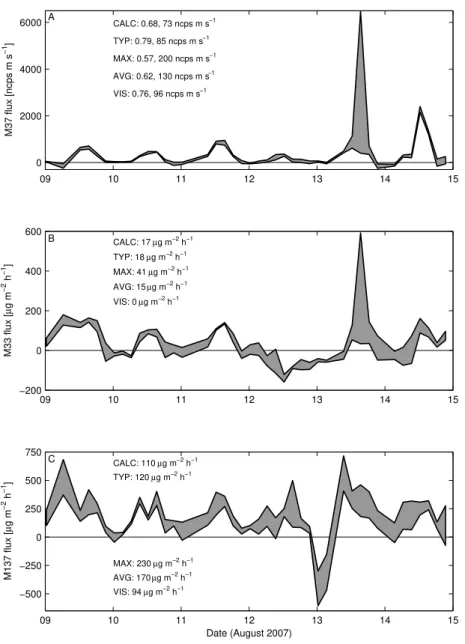
Fig. 6. Range of the M37, M33, and M137 fluxes determined with the five lag time methods (Sect. 2.4). The numbers show the median fluxes and (A) the correlation coefficients between the M37 flux and the reference H2O flux.
the REF box overlap with the notches in the other boxes, the difference between the reference value and each median was not statistically significant at the 95% confidence level. The margin between MAX and CALC as well as MAX and TYP was of borderline significance, otherwise the methods pro-duced quite similar results. The interquartile range (from the 25th to 75th percentile) and the 95% confidence interval of AVG resembled those of REF fairly well. However, the com-parison of the flux statistics did not offer conclusive evidence in favour of or against any of the lag time methods.
In contrast, the error analysis shown in Fig. 5b reveals sub-stantial information on the method performance. To evaluate tendencies to ov or underestimate absolute fluxes, the er-ror had a binary definition. It was defined as the difference
between the simulated DEC flux and the reference EC flux when the reference value was positive or zero. Conversely, the error was the difference between the reference and simu-lated flux when the reference flux was negative.
We can conclude that the median errors of AVG and VIS did not differ from zero at the 95% confidence level. CALC and TYP underestimated the absolute fluxes and MAX was prone to overestimation. As MAX was based on the maximum absolute covariance, it gave rather systemat-ically higher or lower values than the reference depending on the direction of the flux. This overshooting might ex-plain why MAX had such a high median error. Except for one measurement, it could always resolve the flux reliably, in the sense that the absolute flux exceeded the flux uncer-tainty. Rather than providing confidence, this probably just reflects the excess nature of the method.
In summary, the DEC simulation indicated that AVG should be regarded as a promising alternative for lag time determination in DEC measurements. Also VIS can serve as a sound lag time method, provided that the amount of data is reasonable. The overshooting character of MAX may cause a considerable positive bias to the absolute flux in DEC measurements where covariance functions tend to be noisy (Fig. 2).
3.3 Sensitivity of DEC fluxes
Figure 6 illustrates the effect of the lag time methods on the actual DEC measurements with PTR-MS. The flux range due to the methods varied notably during the measure-ment period. It was 20–6100 ncps m s−1 for M37, 6.5– 560 µg m−2h−1for M33, and 18–410 µg m−2h−1for M137. Despite the high momentary deviations, the median fluxes did not differ statistically, except for M137. For it MAX produced a significantly higher result than CALC, TYP, and VIS, while the 95% confidence interval of AVG overlapped with those of all the other methods.
The correlation between the DEC fluxes of M37 and the EC fluxes of H2O was good for each method (Fig. 6a). The correlation coefficient varied between 0.57 and 0.79. The differences were not significant at the 95% level, so the cor-relation analysis did not yield a conclusive result. Like in previous studies (Rinne et al., 2007; Davison et al., 2009), the covariance function of M37 had a visible maximum in most daytime measurements, but the maximum was often in-distinguishable at night. Sometimes VIS failed for M37 but not for M33 and M137, or then their lag times differed sub-stantially (Sect. 3.1). Hence it appears that M37 has limited feasibility to act as a tracer in the lag time determination, de-spite its high potential due to the close correlation with H2O. Although not strictly statistically significant, MAX gave the highest median consistently for M37, M33, and M137. As in the DEC simulation, it produced results that could nearly always be rated reliable. This deceptive feature was again due to the maximum-oriented principle of the method. Based on the flux sensitivity analysis and the DEC sim-ulation, we recommend to be careful when applying MAX to DEC measurements of VOCs. It can cause a remarkable positive bias, even to the median flux, since VOC emission
is normally much higher than deposition. We suggest using AVG instead of MAX as the averaging approach does not have such strong appetite for overestimation. Further, AVG is a convenient alternative to VIS as it makes flux calculation more systematic and less labour-intensive.
4 Conclusions
We presented a straightforward comparison of five lag time methods to assess their applicability to DEC measurements with PTR-MS. According to the DEC simulation, the con-stant lag time methods had a tendency to underestimate the absolute values of fluxes, whereas the maximum covariance method was prone to overestimation. The visual assessment method and the averaging approach did not yield statistically significant errors.
The flux sensitivity analysis indicated that the individual measurements were rather sensitive to the lag time methods, but typically this effect averaged out when the median fluxes were considered. Although not always significant, the max-imum covariance method consistently produced the highest medians, thus reflecting the excess nature of the method. The feasibility of the constant lag time methods was question-able, as expected, due to the substantial lag time variation over time. The variation within compounds illustrated the importance of compound-specific lag time determination.
It would be wrong to advertise our new averaging ap-proach as flawless and beyond compare. However, this study demonstrated that it can reduce the bias somewhat when con-trasted with the customary choice, the maximum covariance method. Given this feature and the potential for automatic flux calculation, we recommend using the averaging method in DEC measurements with PTR-MS.
In principle, the averaging approach is suitable for any eddy covariance application with a low signal-to-noise ra-tio as long as the width of the averaging window is deter-mined properly. Further studies of its performance in dif-ferent micrometeorological conditions and with other com-pounds could reveal new important features.
Acknowledgements. We thank C. Ammann, S. Haapanala, L. J¨arvi, T. Karl, P. Keronen, I. Mammarella, A. Nordbo, and J.-P. Tuovinen for helpful discussions on the many aspects of the lag time challenge. We also thank M. K. Kajos and J. Patokoski for their as-sistance in the DEC measurements. We acknowledge the Academy of Finland (projects 120434, 125238, 209216, and 1118615), the European Integrated Project on Aerosol–Cloud–Climate and Air Quality Interactions (EUCAARI), the Helsinki University Centre for Environment (Urban and Rural Air Pollution Consortium), and the Kone Foundation for financial support.
References
Ammann, C., Brunner, A., Spirig, C., and Neftel, A.: Technical note: Water vapour concentration and flux measurements with PTR-MS, Atmos. Chem. Phys., 6, 4643–4651, doi:10.5194/acp-6-4643-2006, 2006.
Aubinet, M., Grelle, A., Ibrom, A., Rannik, ¨U., Moncrieff, J., Fo-ken, T., Kowalski, A. S., Martin, P. H., Berbigier, P., Bernhofer, Ch., Clement, R., Elbers, J., Granier, A., Gr¨unwald, T., Morgen-stern, K., Pilegaard, K., Rebmann, C., Snijders, W., Valentini, R., and Vesala, T.: Estimates of the annual net carbon and water exchange of forests: The EUROFLUX methodology, Adv. Ecol. Res., 30, 113–175, 2000.
Blake, R. S., Monks, P. S., and Ellis, A. M.: Proton-transfer reaction mass spectrometry, Chem. Rev., 109, 861–896, 2009.
Brunner, A., Ammann, C., Neftel, A., and Spirig, C.: Methanol ex-change between grassland and the atmosphere, Biogeosciences, 4, 395–410, doi:10.5194/bg-4-395-2007, 2007.
Claeys, M., Graham, B., Vas, G., Wang, W., Vermeylen, R., Pashyn-ska, V., Cafmeyer, J., Guyon, P., Andreae, M. O., Artaxo, P., and Maenhaut, W.: Formation of secondary organic aerosols through photooxidation of isoprene, Science, 303, 1173–1176, 2004. Davison, B., Taipale, R., Langford, B., Misztal, P., Fares, S.,
Mat-teucci, G., Loreto, F., Cape, J. N., Rinne, J., and Hewitt, C. N.: Concentrations and fluxes of biogenic volatile organic com-pounds above a Mediterranean macchia ecosystem in western Italy, Biogeosciences, 6, 1655–1670, doi:10.5194/bg-6-1655-2009, 2009.
de Gouw, J. and Warneke, C.: Measurements of volatile organic compounds in the Earth’s atmosphere using proton-transfer-reaction mass spectrometry, Mass Spectrom. Rev., 26, 223–257, 2007.
Guenther, A., Hewitt, C. N., Erickson, D., Fall, R., Geron, C., Graedel, T., Harley, P., Klinger, L., Lerdau, M., McKay, W. A., Pierce, T., Scholes, B., Steinbrecher, R., Tallamraju, R., Tay-lor, J., and Zimmerman, P.: A global model of natural volatile organic compound emissions, J. Geophys. Res., 100(D5), 8873– 8892, 1995.
Guenther, A. B. and Hills, A. J.: Eddy covariance measurement of isoprene fluxes, J. Geophys. Res., 103(D11), 13145–13152, 1998.
Hallquist, M., Wenger, J. C., Baltensperger, U., Rudich, Y., Simp-son, D., Claeys, M., Dommen, J., Donahue, N. M., George, C., Goldstein, A. H., Hamilton, J. F., Herrmann, H., Hoff-mann, T., Iinuma, Y., Jang, M., Jenkin, M. E., Jimenez, J. L., Kiendler-Scharr, A., Maenhaut, W., McFiggans, G., Mentel, Th. F., Monod, A., Pr´evˆot, A. S. H., Seinfeld, J. H., Surratt, J. D., Szmigielski, R., and Wildt, J.: The formation, properties and impact of secondary organic aerosol: current and emerging is-sues, Atmos. Chem. Phys., 9, 5155–5236, doi:10.5194/acp-9-5155-2009, 2009.
Hari, P. and Kulmala, M.: Station for Measuring Ecosystem– Atmosphere Relations (SMEAR II), Boreal Environ. Res., 10, 315–322, 2005.
Hoffmann, T., Odum, J. R., Bowman, F., Collins, D., Klockow, D., Flagan, R. C., and Seinfeld, J. H.: Formation of organic aerosols from the oxidation of biogenic hydrocarbons, J. Atmos. Chem., 26, 189–222, 1997.
H¨ortnagl, L., Clement, R., Graus, M., Hammerle, A., Hansel, A., and Wohlfahrt, G.: Dealing with disjunct concentration
measure-ments in eddy covariance applications: A comparison of avail-able approaches, Atmos. Environ., 44, 2024–2032, 2010. Ibrom, A., Dellwik, E., Larsen, S. E., and Pilegaard, K.: On the
use of the Webb–Pearman–Leuning theory for closed-path eddy correlation measurements, Tellus, 59B, 937–946, 2007. Kaimal, J. C. and Finnigan, J. J.: Atmospheric Boundary Layer
Flows, Oxford University Press, Inc., New York, USA, 1994. Kaimal, J. C. and Gaynor, J. E.: The Boulder Atmospheric
Obser-vatory, J. Clim. Appl. Meteorol., 22, 863–880, 1983.
Karl, T., Guenther, A., Jordan, A., Fall, R., and Lindinger, W.: Eddy covariance measurement of biogenic oxygenated VOC emissions from hay harvesting, Atmos. Environ., 35, 491–495, 2001. Karl, T. G., Spirig, C., Rinne, J., Stroud, C., Prevost, P.,
Green-berg, J., Fall, R., and Guenther, A.: Virtual disjunct eddy covari-ance measurements of organic compound fluxes from a subalpine forest using proton transfer reaction mass spectrometry, Atmos. Chem. Phys., 2, 279–291, doi:10.5194/acp-2-279-2002, 2002.
Keronen, P., Reissell, A., Rannik, ¨U., Pohja, T., Siivola, E.,
Hiltunen, V., Hari, P., Kulmala, M., and Vesala, T.: Ozone flux measurements over a Scots pine forest using eddy covari-ance method: performcovari-ance evaluation and comparison with flux-profile method, Boreal Environ. Res., 8, 425–443, 2003. Kiendler-Scharr, A., Wildt, J., Dal Maso, M., Hohaus, T., Kleist,
E., Mentel, Th. F., Tillmann, R., Uerlings, R., Schurr, U., and Wahner, A.: New particle formation in forests inhibited by isoprene emissions, Nature, 461, 381–384, doi:10.1038/ nature08292, 2009.
Koppmann, R., ed.: Volatile Organic Compounds in the Atmo-sphere, Blackwell Publishing Ltd, Oxford, UK, 2007.
Lenschow, D. H., Mann, J., and Kristensen, L.: How long is long enough when measuring fluxes and other turbulence statistics?, J. Atmos. Ocean. Tech., 11, 661–673, 1994.
Lindinger, W., Hansel, A., and Jordan, A.: On-line monitoring of volatile organic compounds at pptv levels by means of Proton-Transfer-Reaction Mass Spectrometry (PTR-MS) – Medical ap-plications, food control and environmental research, Int. J. Mass Spectrom., 173, 191–241, 1998.
Markkanen, T., Rannik, ¨U., Keronen, P., Suni, T., and Vesala, T.: Eddy covariance fluxes over a boreal Scots pine forest, Boreal Environ. Res., 6, 65–78, 2001.
Massman, W. J.: A simple method for estimating frequency re-sponse corrections for eddy covariance systems, Agr. Forest Me-teorol., 104, 185–198, 2000.
McGill, R., Tukey, J. W., and Larsen, W. A.: Variations of box plots, Am. Stat., 32(1), 12–16, 1978.
McMillen, R. T.: An eddy correlation technique with extended applicability to non-simple terrain, Bound.-Lay. Meteorol., 43, 231–245, 1988.
M¨uller, M., Graus, M., Ruuskanen, T. M., Schnitzhofer, R., Bam-berger, I., Kaser, L., Titzmann, T., H¨ortnagl, L., Wohlfahrt, G., Karl, T., and Hansel, A.: First eddy covariance flux mea-surements by PTR-TOF, Atmos. Meas. Tech., 3, 387–395, doi:10.5194/amt-3-387-2010, 2010.
Rinne, H. J. I., Guenther, A. B., Warneke, C., de Gouw, J. A., and Luxembourg, S. L.: Disjunct eddy covariance technique for trace gas flux measurements, Geophys. Res. Lett., 28(16), 3139–3142, 2001.
fluxes above a Scots pine forest canopy: measurements and mod-eling, Atmos. Chem. Phys., 7, 3361–3372, doi:10.5194/acp-7-3361-2007, 2007.
Rinne, J., Douffet, T., Prigent, Y., and Durand, P.: Field comparison of disjunct and conventional eddy covariance techniques for trace gas flux measurements, Environ. Pollut., 152, 630–635, 2008. Shaw, W. J., Spicer, C. W., and Kenny, D. V.: Eddy correlation
fluxes of trace gases using a tandem mass spectrometer, Atmos. Environ., 32, 2887–2898, 1998.
Shimizu, T.: Practical applicability of high frequency correction
theories to CO2flux measured by a closed-path system,
Bound.-Lay. Meteorol., 122, 417–438, doi:10.1007/s10546-006-9115-z, 2007.
Spirig, C., Neftel, A., Ammann, C., Dommen, J., Grabmer, W., Thielmann, A., Schaub, A., Beauchamp, J., Wisthaler, A., and Hansel, A.: Eddy covariance flux measurements of biogenic VOCs during ECHO 2003 using proton transfer re-action mass spectrometry, Atmos. Chem. Phys., 5, 465–481, doi:10.5194/acp-5-465-2005, 2005.
Su, H.-B., Schmid, H. P., Grimmond, C. S. B., Vogel, C. S., and Oliphant, A. J.: Spectral characteristics and correction of long-term eddy-covariance measurements over two mixed hardwood forests in non-flat terrain, Bound.-Lay. Meteorol., 110, 213–253, 2004.
Taipale, R., Ruuskanen, T. M., Rinne, J., Kajos, M. K., Hakola, H., Pohja, T., and Kulmala, M.: Technical Note: Quantitative long-term measurements of VOC concentrations by PTR-MS – measurement, calibration, and volume mixing ratio calculation methods, Atmos. Chem. Phys., 8, 6681–6698, doi:10.5194/acp-8-6681-2008, 2008.
Turnipseed, A. A., Pressley, S. N., Karl, T., Lamb, B., Nemitz, E., Allwine, E., Cooper, W. A., Shertz, S., and Guenther, A. B.: The use of disjunct eddy sampling methods for the determination of ecosystem level fluxes of trace gases, Atmos. Chem. Phys., 9, 981–994, doi:10.5194/acp-9-981-2009, 2009.
Warneke, C., Luxembourg, S. L., de Gouw, J. A., Rinne, H. J. I., Guenther, A. B., and Fall, R.: Disjunct eddy covariance measure-ments of oxygenated volatile organic compounds fluxes from an alfalfa field before and after cutting, J. Geophys. Res., 107(D8), 4067, doi:10.1029/2001JD000594, 2002.
Wienhold, F. G., Frahm, H., and Harris, G. W.: Measurements of N2O fluxes from fertilized grassland using a fast response