www.hydrol-earth-syst-sci.net/18/2141/2014/ doi:10.5194/hess-18-2141-2014
© Author(s) 2014. CC Attribution 3.0 License.
A prototype framework for models of socio-hydrology:
identification of key feedback loops and parameterisation approach
Y. Elshafei1, M. Sivapalan2,3, M. Tonts1, and M. R. Hipsey1
1School of Earth & Environment, The University of Western Australia, Crawley WA 6009, Australia
2Department of Civil and Environmental Engineering, University of Illinois at Urbana-Champaign, N. Mathews Avenue, Urbana, IL 61801, USA
3Department of Geography and Geographic Information Science, University of Illinois at Urbana-Champaign, Computing Applications Building, Springfield Avenue, Urbana, IL 61801, USA
Correspondence to:Y. Elshafei ([email protected])
Received: 15 December 2013 – Published in Hydrol. Earth Syst. Sci. Discuss.: 14 January 2014 Revised: 30 April 2014 – Accepted: 8 May 2014 – Published: 13 June 2014
Abstract. It is increasingly acknowledged that, in order to
sustainably manage global freshwater resources, it is criti-cal that we better understand the nature of human–hydrology interactions at the broader catchment system scale. Yet to date, a generic conceptual framework for building models of catchment systems that include adequate representation of socioeconomic systems – and the dynamic feedbacks be-tween human and natural systems – has remained elusive. In an attempt to work towards such a model, this paper outlines a generic framework for models of socio-hydrology appli-cable to agricultural catchments, made up of six key com-ponents that combine to form the coupled system dynamics: namely, catchment hydrology, population, economics, envi-ronment, socioeconomic sensitivity and collective response. The conceptual framework posits two novel constructs: (i) a composite socioeconomic driving variable, termed the Com-munity Sensitivity state variable, which seeks to capture the perceived level of threat to a community’s quality of life, and acts as a key link tying together one of the fundamental feedback loops of the coupled system, and (ii) a Behavioural Response variable as the observable feedback mechanism, which reflects land and water management decisions rele-vant to the hydrological context. The framework makes a further contribution through the introduction of three macro-scale parameters that enable it to normalise for differences in climate, socioeconomic and political gradients across study sites. In this way, the framework provides for both macro-scale contextual parameters, which allow for comparative studies to be undertaken, and catchment-specific conditions,
by way of tailored “closure relationships”, in order to ensure that site-specific and application-specific contexts of socio-hydrologic problems can be accommodated. To demon-strate how such a framework would be applied, two socio-hydrological case studies, taken from the Australian experi-ence, are presented and the parameterisation approach that would be taken in each case is discussed. Preliminary find-ings in the case studies lend support to the conceptual theo-ries outlined in the framework. It is envisioned that the appli-cation of this framework across study sites and gradients will aid in developing our understanding of the fundamental in-teractions and feedbacks in such complex human–hydrology systems, and allow hydrologists to improve social–ecological systems modelling through better representation of human feedbacks on hydrological processes.
1 Introduction
The history of mankind can be written in terms of human interactions and interrelations with water. (Biswas, 1970)
that water, unlike oil, has no viable substitutes for human-ity. As a result of growing populations, rapid and exten-sive industrialisation, and over-allocation and mismanage-ment of freshwater resources, a looming global water crisis that is said to be “unprecedented in human history” has been predicted (Falkenmark, 1997; Biswas, 1999; Postel, 2003; Pearce, 2007; Barlow, 2007; Biswas and Tortajada, 2011; Fishman, 2011).
It is widely recognised in the field of hydrology that human actions have myriad impacts on hydrological dynamics at the catchment system scale, including via land use changes, the alteration of flow regimes through the construction of dams and weirs, the deterioration of water quality through the pol-lution of waterways, as well as numerous impacts on biogeo-chemical cycles and riverine and lake ecology (Carpenter et al., 2011; Montanari et al., 2013). Similarly, it is acknowl-edged in the social sciences that the well-being of human societies is extraordinarily dependent upon what has been termed the “planet’s life-support system”, not only in terms of global water needs, but also with respect to its role in food production, poverty alleviation, energy production, hu-man health, transport, climate regulation and ecosystem ser-vices (Falkenmark, 2001, 2003). Falkenmark (2003, p. 2038) makes the point that “to support the growing world popu-lation, balancing will be needed between emerging societal needs and long-term protection of the life-support system upon which social and economic development ultimately de-pends”. This sentiment is echoed in numerous other studies (Biswas, 1997; Folke, 1998; Rockström et al., 2007, 2009; Varis, 2008). To date, major advances in the disciplines of hydrological sciences and water resources management have helped us understand these challenges, yet it remains critical that we better characterise and quantify the dynamic nature of human–hydrology interactions, in order that we can effec-tively manage them in a sustainable manner (Montanari et al., 2013; Thompson et al., 2013).
Notwithstanding that the dynamic interconnection of human and natural systems has long been documented (e.g. Marsh, 1864; Thomas Jr., 1956; Falkenmark, 1979; Turner et al., 1990; McDonnell and Pickett, 1993; Kates and Clark, 1999), a practical understanding of the complex co-evolution processes and interactions therein is still limited (Low et al., 1999; Kinzig, 2001; Liu et al., 2007a). Integrated Water Resources Management (IWRM) has historically been the framework within which interactions between human de-velopment and water resources have been explored. The lim-itation of such an approach is that the examination of single system components in isolation, such as treating scenario-based water management solutions as boundary conditions to hydrological models, is insufficient to capture the more infor-mative co-evolving coupled dynamics and interactions over long periods (Liu et al., 2008; Sivapalan et al., 2012). As a re-sult of this knowledge gap, interdisciplinary research efforts have emerged, such as the Coupled Human and Nature Sys-tems (CHANS) (Liu et al., 2007a, b) and Social-Ecological
Systems (SES) communities (Berkes and Folke, 1998). The focus of these efforts is on furthering our understanding of the complex interactions within the continually evolving cou-pled system, in terms of the feedbacks, nonlinearities, thresh-olds, transformations and time lags. As observed by Schlüter et al. (2012, p. 221), “while the importance of the human di-mension and social dynamics for sustainable resource man-agement is well recognised, the uncertainty generated by human responses to institutional or environmental change has only received limited attention so far”. The need for a prescriptive conceptual framework which seeks to examine complex dynamics resulting from interactions and feedbacks between agents, resources and institutions on multiple levels has been highlighted (Berkes and Folke, 1998; Anderies et al., 2006b), with the caveat that “any theory devised to un-derstand SESs. . . would span cognitive science, psychology, economics, ecology, biogeochemistry, mathematics, physics, etc.” (Anderies et al., 2006b, p. 1). In spite of the seemingly Herculean task at hand, several recent important strides have been made to this end (Schlüter and Pahl-Wostl, 2007; Os-trom, 2009; Epstein et al., 2013; Lade et al., 2013; Schlüter et al., 2013). An excellent review of SES model applications using a host of different approaches within various fields of research, including fisheries, rangelands, wildlife, ecological economics and resilience and complex systems theory, can be found in Schlüter et al. (2012).
interactions (Di Baldassarre et al., 2013a, b), urban water security (Srinivasan, 2013), and downstream use of glacier runoff (Carey et al., 2014), while others have focused on tai-lored case-specific coupled model formulations (Liu et al., 2014; Pande et al., 2013; van Emmerik et al., 2014).
The development of a robust internationally applicable theoretical framework that has the capacity to guide the for-mulation of localised socio-hydrology models is needed for application across diverse study sites and application con-texts. In doing so, such a framework can draw on emerg-ing themes in the social sciences and SES literature to aug-ment current directions in hydrology research. The resultant framework would enable extensive empirical examination of co-evolving dynamics across climate, socioeconomic and po-litical gradients, with the ultimate aim of identifying underly-ing fundamental principles inherent in the integrated system. Given the challenging nature of the exercise, in order to begin to detect certain key feedbacks and drivers in a highly complex coupled system, as a starting point this paper out-lines a model framework within the context of catchments that are simplified “uni-dimensional” systems in terms of economic activity and development. In light of the fact that agriculture now covers almost 40 % of the world’s terres-trial surface and accounts for approximately 85 % of global consumptive freshwater use (Foley et al., 2005; Carpenter et al., 2011), it is especially pertinent to examine agricul-turally focused catchments given their global footprint. As a result of changes in land use, land cover and irrigation, agri-culture has significantly transformed the global hydrological and ecological cycles (Gordon et al., 2010), with some stud-ies documenting co-evolutionary dynamics (e.g. Anderstud-ies et al., 2006a; Kandasamy et al., 2014), thus making it an ideal focus for the study of socio-hydrology.
This paper therefore outlines a conceptual framework to examine the coupled dynamics of integrated agricultural socio-hydrology catchment systems. The paper proposes a composite socioeconomic driving variable that acts as the missing link tying together one of the key feedback loops of the socio-hydrology system. It goes on to specify six key functional components of the generic framework, showing the flexibility inherent therein to account for both the macro-scale context, as well as unique catchment-specific aspects, which can be captured through locally tailored “closure rela-tionships”. The paper concludes by demonstrating how such a framework would be applied to two site-specific Australian case studies, with a discussion on the parameterisation ap-proach and characterisation of closure relationships for each.
2 Conceptual basis for a model of socio-hydrology
The conceptual framework put forward in this paper is a nec-essary simplification of an extremely complex coupled sys-tem. The intention however, is to build an approach able to support a grassroots understanding of how the coupled
sys-tem might function, and to stress-test certain basic assump-tions prior to progressing to more advanced and fully pa-rameterised models. We can thus begin to comprehend the crucial components, flows, nonlinear interactions, feedbacks and responses of key system attributes that are essential steps in the development of models for interdisciplinary and com-plex problems (Heemskerk et al., 2003; Schlüter et al., 2012). It is well established in the resilience literature that change (whether drastic or incremental) acts as a catalyst to response (e.g. Forbes et al., 2004; Dale et al., 2010). The question is, what magnitude of change in what composite of factors is sufficient to drive a measurable reaction in the first in-stance? Furthermore, once a response is invoked, what are the determinants of the immediacy and degree of that re-sponse, and what, if any, are the lagged responses? Marginal changes in the social, economic and environmental compo-nents of the socio-hydrological system may be driven by ex-ogenous factors external to the catchment (e.g. climate, mar-ket prices and demand, political changes) or endogenous fac-tors generated by internal feedbacks within the catchment (as stipulated in the assumptions and component equations of the model framework). Such changes invariably feed back to the hydrological sub-system via a behavioural response from the human sub-system, since humans will change the rate at which they interact with the catchment water balance. In this way, the two sub-systems are perpetually co-evolving through time, and this forms the basic premise of the pro-posed framework. The fundamental question we are moti-vated to answer through application of a socio-hydrological model is whatdrivesthe human response within the human sub-system. As outlined above, the impacts of land and water management decisions on the hydrological system, in terms of water balance, flows and quality, are presently well un-derstood and modelled. However, thedrivers of the human feedback component at a system scale have remained elusive. The goal of a socio-hydrology model is therefore to identify, conceptualise and eventually quantify these drivers, so as to formulate generalised principles that will form the basis of a broadly applicable coupled model.
Catchment
Economics:
GDP perp capitap
Productive
Land, Water Population
Environment/
Ecosystem Services
Quantity &
Quality
Population
Size &
Growth
Climate Regime/ Scale
Demand for
Behavioural
Community
Sensitivity
Socioeconomic
Regime/ Scale Macro‐scale
Normalising
Factors
Water Response
Political
Regime/ Scale
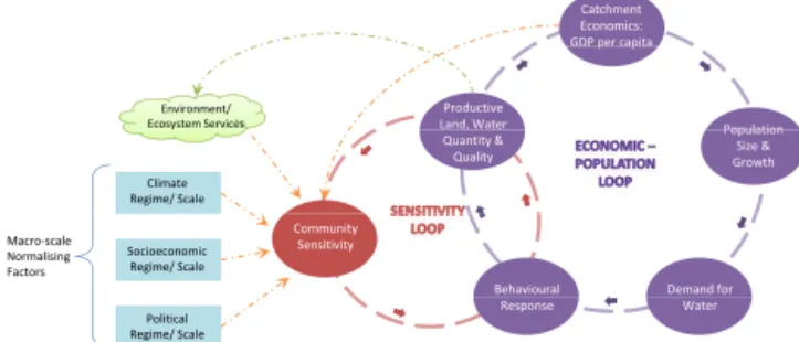
Figure 1.The socio-hydrology model as two interconnecting
feed-back loops.
catchment states defined by water availability (ST), degraded land (AD)and catchment GDP (EC)could potentially show a catchment moving from state 1 point of “highST–lowAD– lowEC” to state 2 of “lowST–highAD–highEC”. Negative feedbacks will stabilise the system such that it will resist be-ing pushed away from its original position. However, positive feedbacks and unstable dynamics will induce a shift to the second position. The three key emergent properties we seek to understand in the interaction of the socio-hydrological system from a systems perspective are (1) the resilience of the system in terms of its stability and threshold behaviour from one state to another, and in so doing to gauge the na-ture and magnitude of negative and positive feedbacks, re-spectively, (2) the differences in timescales and inherent lags between system interactions and feedbacks, and (3) the de-gree of adaptation and learning intrinsic to the human system (Allison and Hobbs, 2004; Gunderson and Holling, 2002). These behaviours are what we are aiming to investigate with the socio-hydrology model in order to better understand the workings of the coupled system. Understanding these key system features, as well as the system variables that charac-terise its dynamics, would enable targeted policies and man-agement strategies that promote sustainable water resource management, especially with respect to case studies at ear-lier stages of the evolving cycle.
2.1 The two key feedback loops
In this section we highlight two principal feedback loops that emerge in the dynamics of the coupled system (Fig. 1). The first is referred to as the “Economic-Population Loop” and the second as the “Sensitivity Loop”. With respect to the former, the increasing trend in global water use has been closely linked to both population growth and economic de-velopment over the past few centuries (Vörösmarty et al., 2005). If we take a pristine catchment (pre-human influ-ence) we would observe certain hydrological variables as a result of its climate and geophysical make-up. These ef-fectively determine the initial condition for available water quantity and quality. A certain proportion of this available water would be employed towards economic gain (for
ex-ample, for normal household use and agriculture). This eco-nomic gain would be distributed (often unequally) on a per capita basis throughout the catchment community. It follows that, as the per capita economic gain increases, the catch-ment presents a more attractive lifestyle proposition caus-ing a net migration of people into the catchment, such that population size would increase, as well as its rate of growth, similar to Myrdal’s (1957) concept of “circular and cumu-lative causation”. A growing population would be accom-panied by higher levels of demand for water and land, by virtue of increased household consumption and a growing requirement for economic development to sustain the larger community (Molle, 2003). In addition, as a rural catch-ment with a predominantly agricultural micro-economy in-creases in prosperity, water demand will originate from addi-tional sources independent of population growth, to a point, e.g. from the manufacturing sector, thermoelectric sector and increasingly sophisticated domestic household needs (as ob-served by Flörke et al., 2013).
This heightened demand is likely to be one of the key drivers feeding into water management decisions, such as extraction rates, land clearance rates and the construction of storage facilities. Management decisions would be reflected in the community’s economic prosperity in the short term, and filter through to water quantity and quality variables over a longer timescale. From this point, the water variables can be viewed more as limiting variables or lower boundary con-ditions, whereby economic growth will continue to be pos-sible until such time that the quantity or quality of natural resources impede further growth. Water use efficiency mea-sures would feed into the cycle to extend the life or eco-nomic productivity of these limiting variables. However, to the extent that water flows reduce, water quality deteriorates or land degrades, economic growth will naturally be con-strained. In the case of common pool resources, the resource that underpins development, in this case the freshwater re-source, is often prone to over-exploitation, which can ulti-mately lead to a deterioration in local social and economic conditions (Hardin, 1968). This will in turn encourage migra-tion out of the catchment as people go in search of other work and income opportunities, which will in turn reduce the de-mand for water and land. Management decisions might then reasonably respond by reducing extraction rates and environ-mental restoration. This is the first feedback loop that merits investigation.
exposureto change (whether drastic or gradual) in the socio-hydrological system is captured by the primary sub-system functions originating from a change in the land and water variables; thesensitivityto that exposure is what we seek to capture in our sensitivity variable; while the demonstrated resilienceof the system is effectively reflected within a be-havioural response function that drives actual change within the catchment (further discussed in Sect. 3.6).
The underlying premise of the Sensitivity Loop is that be-haviour and water management decisions are directly driven by a community’s social and environmental values, local ac-tion, lobbies and the like, all of which reflect community sen-sitivity to direct and indirect impacts of a marginal change in one or more of the water variables. The behavioural response, as before, will impact future available water quantity and quality. The proposition in this paper is that as the Sensitivity state variable displays an upward or downward shift, there will be a corresponding observable shift in a Behavioural Response function. It is hypothesised that as Sensitivity in-creases, behaviour and management decisions will tend to-wards reducing the community’s impact on the basin’s hy-drological signature (i.e. a move towards a more natural en-vironment). Conversely, lower sensitivity rates will be asso-ciated with more aggressive behavioural responses that tend towards manipulating available water resources to the com-munity’s needs (i.e. a more observable anthropogenic foot-print).
The assumption of rational behaviour in this context per-tains to the likelihood that overarching community behaviour will tend towards the longer-term collective good, rather than the short-term individual good. One of the challenges asso-ciated with the management of water resources is that it is a common pool, open access resource, and as a consequence it is potentially prone to overharvesting as individuals seek to optimise use, otherwise known as the “tragedy of the com-mons” (Hardin, 1968). In recent decades however, the pre-diction of collective over-exploitation of the resource under the rational-agents paradigm has been called into question (Ostrom et al., 2002). It has become increasingly apparent that such individual optimisation is not always the case, and that in fact the degree of collective co-operation in commons dilemmas is influenced by both micro-situational variables (e.g. heterogeneity among agents, group size, communica-tion, reputacommunica-tion, time horizons) and the broader context (An-deries and Janssen, 2011; Tavoni et al., 2012; An(An-deries et al., 2013). This is in line with Giddens’ (1984) early work on structuration theory, which posits that social phenomena are the result of both agency and social structure. Indeed, Kinzig et al. (2013) note that as adopters of a particular behaviour reach a critical quorum, which may be as few as 10 % of the population, a tipping point may be reached that causes the new norms to be more widely adopted by the commu-nity, such that a collective move towards more environmen-tally sustainable practices occurs. Thus, a composite variable based on collective community sensitivity as a driver to
co-
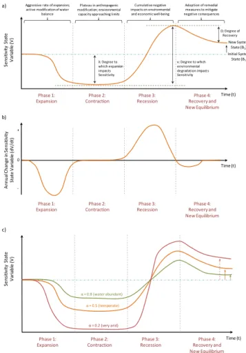
Phase 1: Expansion
Time (t)
S e n sit iv it y St a te Va ri a b le (V )
Initial System
State (B1) New System
State (B2)
Phase 2: Contraction Phase 3: Recession Phase 4: Recovery and New Equilibrium
: Degree to
which expansion
impacts
Sensitivity Aggressive rate of expansion;
active modification of water
balance
Plateau in anthropogenic
modification; environmental
capacity approaching limits
Cumulative negative
impacts on environmental
and economic well‐being
Adoption of remedial
measures to mitigate
negative consequences
: Degree to which
environmental
degradation impact s
Sensitivity
Ω: Degree of
Recovery
Time (t)
An n u a l Ch a n ge in S e n sit iv it y Sta te Va ri a b le (d V/ d t) + ‐ 0 Phase 1:
Expansion ContractionPhase 2:
Phase 3: Recession Phase 4: Recovery and New Equilibrium a) b) Phase 1: Expansion
Time (t)
S e n sit iv it y St a te Va ri a b le (V )
α= 0.5 (temperate)
Phase 2: Contraction Phase 3: Recession Phase 4: Recovery and New Equilibrium
α= 0.2 (very arid)
α= 0.8 (water abundant)
c)
Figure 2.An idealised sketch showing a hypothetical trajectory
over time for the(a)Sensitivity state variable, and(b)the change in
SensitivitydVdtin the case of an example catchment. A
compar-ison of the idealised trajectory across a regional climate gradient is shown in(c).
operative action is achievable with the use of agent-based models (Tavoni et al., 2012) that would account for the di-versity of actions by individual actors within the catchment community.
of as the positive feedback loop indicative of the Economic-Population Loop described in Fig. 1. The third phase (Reces-sion) is comprised of a sharp cumulative decline in the con-dition of environmental resources, accompanied by a down-turn in economic prosperity linked to the resource degrada-tion. The negative feedbacks inherent in the Sensitivity Loop take effect during this phase. The fourth phase (Recovery and New Equilibrium) is characterised by a shift in behaviour patterns towards enviro-centric management and policy fo-cused on alleviating the negative consequences of a legacy of expansion. The system shifts to a new equilibrium state (B2), that may then be subject to a relatively small magnitude of oscillation beyond this point. There are numerous examples in the literature where this pattern of a positive feedback loop followed by a negative feedback loop (i.e. aggressive devel-opment followed by remedial management efforts) has been observed in local and regional-scale socio-hydrological sys-tems: the Saskatchewan River basin in Canada (Gober and Wheater, 2014), the Tarim River basin in China (Liu et al., 2014), the Murrumbidgee River basin in eastern Australia (Kandasamy et al., 2014), the West Australian “Wheatbelt” (Allison and Hobbs, 2004), the California Delta in the US (Norgaard et al., 2009) and several other basins around the world (Molden et al., 2001; Molle, 2003; Vörösmarty et al., 2005; Kinzig et al., 2006; Savenije et al., 2014). Indeed, these dynamics have also been observed at a larger global system scale (Cosgrove and Rijsberman, 2000). We acknowledge that Fig. 2 is hypothetical and real-world cases will exhibit departures from the idealised trajectory depicted.
2.2 Identifying the missing link: community sensitivity
as a state variable
A clear starting point in the development of a systems model spanning water resources and human activity requires the definition of a set of state variables and the core “curren-cies” of the model. In general terms, these relate to: (a) water availability and environmental quality, (b) economic value of the catchment system, and (c) social and population dynam-ics and structure. However, the challenge in modelling both socioeconomic and hydrological systems is that it is difficult to define what connects this collection of catchment system variables.
In the framework, we propose a composite driving state variable that can be thought of as the community’s sensitiv-ity to a change in hydrological variables, as it begins to man-ifest in associated economic and environmental variables. In the simplest sense, the greater the collective sensitivity, the greater will be the stimulus to take enviro-centric action (Falkenmark, 1997; Folke et al., 2010) and this creates a neg-ative feedback that will promote stability. Likewise, the lower the sensitivity, the less likelihood that a change in hydrolog-ical variables will lead to meaningful enviro-centric action, and the population will continue to drive the system towards a different state-space location that may be more or less
sustainable. The drivers of collective human values, emo-tions, perceptions and behaviour, already forms a body of research within the psychology and natural resource manage-ment fields, with myriad theories and ongoing debate (Ajzen, 1985; Broderick, 2007; Stein et al., 1999; Vanclay, 1999, 2004; Vaske and Donnelly, 1999; Armitage and Christian, 2003; Seymour et al., 2010; Mankad, 2012). This paper does not aim to contribute to these debates. Rather, from a purely socio-hydrological context, we are seeking to simplify these drivers into observable proxies that enable an understanding of how the coupled system interacts. We define these prox-ies as socio-hydrological “closure relationships”, which refer to the formalisation of certain contextually-specific relation-ships with mathematical functions in order to fully resolve interdependencies required to make equations determinate.
This paper puts forward the suggestion that a community’s sensitivity stems from its perceived level of threat to its qual-ity of life, which could also be thought of in terms of a dis-ruption to its established norms and behaviours (Kinzig et al., 2013). The more a community perceives its quality of life to be under threat, the more likely it is to display heightened sensitivity to a marginal change in factors that could sub-sequently negatively impact its quality of life. Conversely, the less a community perceives its quality of life to be under threat, the less likely it is to be sensitive (and hence react) to marginal changes in such variables. In this way, the sensi-tivity is related to how any marginal change in hydrological variables manifests itself in the economic, social and envi-ronmental dimensions that more directly pertain to a com-munity’s overall quality of life. Indeed, there is evidence to support the notion that the behaviour of a watershed commu-nity, with respect to water management, is dependent upon its heldperceptionsof the severity and magnitude of prob-lems it faces (Molle, 1991, 2003; Turral, 1998; Zilberman et al., 2011). Although most of this literature addresses re-sponse management to severe water shortages or disasters, these are still extreme manifestations of the inherent causal link between perceptions of threat and action.
evidence in the literature to support the view that people’s perceptions and propensity to act are directly related to their degree of physical proximity and personal experience with the issues faced. Put another way, people tend to be most sensitive to those things that impactdirectlyupon their qual-ity of life (Kollmuss and Agyeman, 2002; Rolfe et al., 2005; Broderick, 2007; Gooch and Rigano, 2010).
Resilience, in its traditional sense, hinges upon the notion of positive, adaptive responses that may be preventative or responsive in nature, in order to avoid or moderate negative consequences (Masten et al., 1990; Luthar et al., 2000). Al-though the concept of resilience originated in the ecological sciences (Holling, 1973) it has been found to be particularly useful in the examination of coupled human–nature system studies (Berkes and Folke, 1998; Berkes and Jolly, 2002; Berkes et al., 2003; Falkenmark, 2003; Folke, 2003; Anderies et al., 2004; Folke, 2006; Forbes et al., 2009; Amundsen, 2012). Whether used in the field of psychology, ecology or social science, the concept is based upon the premise of a system’s response tochange. Negative consequences in our model are analysed with respect to the catchment commu-nity’s quality of life. Given that sensitivity, as applied in this paper, is essentially a subjective variable, it could prove ulti-mately impossible to quantify in absolute terms in any widely applicable way. This paper therefore posits the use of a rel-ative scale. In this way, the scale would reflect a marginal change, as opposed to reporting an absolute value, thus shift-ing the focus to the direction and relative magnitude of any movement.
From a model standpoint, the overall objective is to de-velop a lifestyle sensitivity variable that is capable of ade-quately capturing a community’s shifting perception of its own vulnerability, such that it is a reasonable precursor to observable action. Community perceptions have generally been canvassed using qualitative means (i.e. interviews, sur-veys) as it is an inherently subjective trait (Broderick, 2007; Guimarães et al., 2012; Tolun et al., 2012). Given that it is only possible to canvass perceptions in this manner at a given point in time, we are precluded from doing this in the present context as we are attempting to capture phenomena and feed-backs over historical periods of a century or more. At present, there is no prescriptive method for quantifying or modelling human perceptions to changes in their environment (environ-mental, social, economic or otherwise) (Jones et al., 2011; Lynam and Brown, 2012) and we therefore resort to proxies (discussed in more detail in Sect. 3.5). However, it is conceiv-able that at some point in the future, advancements in mental models research will enable the substitution of a more so-phisticated parameterisation of our sensitivity variable.
3 The six key components of a generic framework
The conceptual foundations outlined above are used to un-derpin the construction of a prescriptive socio-hydrology
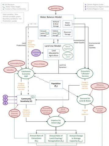
Rainfall/ QET
Water Balance Model:
Wetland
& Ri Water
α: Climate Regime Scalar
β: Socioeconomic Regime Scalar
φ: Political Regime Scalar
θ: Soil Moisture
hWT: Water Table Height
ω: Fraction of Non‐Conformists
State variables : blue
Derived variables: green
Boundary conditions: red
Parameters: purple
Ground water Storage Vadose Zone Storage Reservoir Storage & River
Storage Quality
Environmental
Water Quality Environmental
Land
Change in
Water
Availability
θ hWT
Land Use Model:
Catchment
Area
Land
Allocated to
Agriculture DegradedLand
Commodity Price
Water
Quantity Productivity
Price of Water Availability
over time Native
Vegetation Land Use Catchment Economic GDP Ecosystem “Lifestyle” Services Population (P )
Change in
Ecosystem
Services Change in
Economic
Land Use
Dynamics
Efficiency
Subsidies
Community Sensitivity (V)
Demand for Land & Water (Pn)
α β φ
Services
over time Productivity
over time
Improvements ω Social Cohesion Impetus for Action (Δχ) Economic Development Quotient Demand for Expansion Change in
Community
Sensitivity
over time Economic Diversity Quotient Economic Growth Annual Rate of Extractions
(RE)
Annual Change in Storage Capacity (Smax) Annual Rate of
Land Clearing/ Revegetation (AC)
Figure 3.A generic socio-hydrology conceptual framework for
ap-plication to agricultural catchments.
framework for application to agricultural catchments. The framework in a generic form consists of six components that together combine to form a coupled system capturing the feedbacks previously highlighted (Fig. 3). The follow-ing section describes each of the main framework compo-nents with discussion of associated functional relationships that are required to be parameterised (the reader is referred to Appendix A for a complete list of variables and associated measurement units). The first four components can be mod-elled in numerous ways, with the level of complexity inherent in the chosen method up to individual practitioners to deter-mine, depending on the relative importance of each aspect to the investigation at hand. However, to demonstrate how the framework would be applied, we have sketched some generic basic concepts that could be applied to realise each compo-nent.
3.1 Catchment hydrology
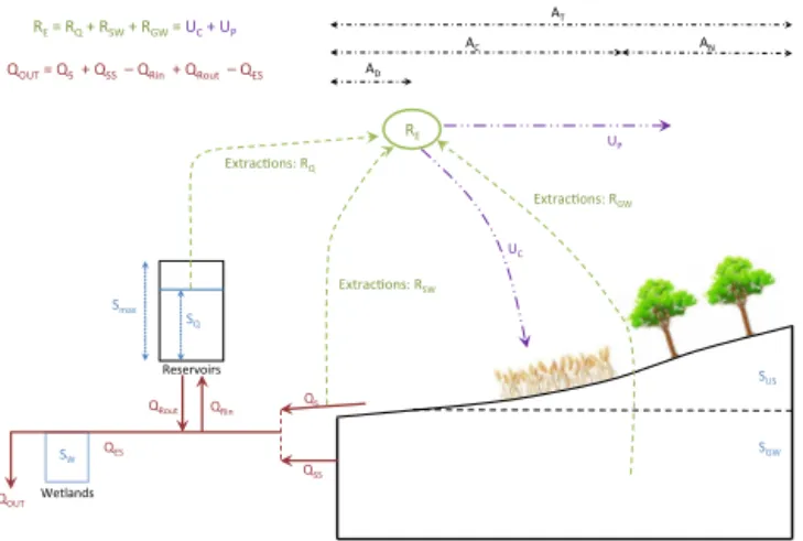
SUS
SGW SW
SQ Smax
AT
AC AN
AD
QOUT
QS
QSS QRin QRout
QES
Reservoirs
Extrac<ons: RGW
Extrac<ons: RSW Extrac<ons: RQ
Wetlands
QOUT = QS + QSS – QRin + QRout – QES
RE = RQ + RSW + RGW = UC + UP
UC
UP RE
Figure 4.A simple catchment water balance model that includes
the minimum necessary components for application of the
concep-tual framework. Groundwater (SGW), vadose zone (SUS), wetland
(SW) and reservoir (SQ) water stores are included. Cumulative
man-made storage capacity (Smax) must also be included. Net flows
(QOUT) are modelled using surface flow (QS), subsurface flows
(QSS), managed diverted (QRin) and released (QRout) flows, and
environmental flows (QES). Managed extractions made from the
system from each of groundwater (RGW), surface (RSW) and
reser-voir (RQ) sources must be accounted for. Land use decisions must
also be reflected, such that area of land cleared (AC), area of
remain-ing land comprised of natural vegetation (AN) and area of degraded
land (AD) must form a dynamic part of the model.
on the basic geophysical properties of the catchment, climate forcing, and also allow for anthropogenic influences on the hydrological signature of the basin. For most cases a model setup where the catchment is divided into sub-catchments (i.e. semi-distributed) with each accounting for dynamics of soil moisture, groundwater stores, evapotranspiration and surface water runoff and routing or storage (as relevant) would be suitable. Where the underlying socio-hydrologic case study requires resolution of changes to water quality, then this model must be extended to simulate water quality dynamics.
For the purposes of this paper, the specification of the wa-ter balance model is only covered in general wa-terms, as de-picted in Fig. 4, and individual case study applications of the framework would require contextually relevant imple-mentations. The key attributes the model must have however, to support simulation of the coupled dynamics, is to allow for a link to water-related management decisions relevant at the catchment system scale. These include ability to accom-modate within the catchment water balance: (i) changes in land cover (AC; e.g. due to clearing of native vegetation), (ii) changes in the rate of extractions of either surface water or groundwater for economic activity (RE), and (iii) changes in the capacity for water storage (Smax; e.g. development or removal of reservoirs or other forms of river regulation). Based on behavioural responses outlined below, these three
mechanisms form the core links that allow the water balance to be modified by the catchment population.
3.2 Population dynamics
The Demographic Transition Model has been used exten-sively to model the relationship between development and population in human geography (Jones, 2012), and may be employed to calculate the catchment population. This ap-proach bases population dynamics on changes in the birth rate and death rate as a country moves through five different stages of development. Extensions and variations of the core model have been developed for various countries, which al-low the potential for more tailored versions of the model to be applied. In addition to the birth rate and mortality rate, the net permanent migration rate can be calculated by accommo-dating various “push” and “pull” factors that focus on local economic, environmental and political conditions (Fouberg et al., 2010). In general terms, the population state variable,
Pn, would evolve according to
dPn
dt =(b−m+µ)Pn, (1)
whereb is the annual birth rate, mis the annual mortality rate, and µ is the annual net migration rate. Migration is driven by a wide range of local and external factors and is beyond the scope of this paper to cover in detail, however depending on the application context, it could be driven by internally derived variables related to the catchment system, for example, economic benefit of crop production or ecosys-tem services and conditions that support a high quality of life. Additional factors such as natural (e.g. earthquakes, drought) and man-made (e.g. war) hazards could act as “push” factors. Various applications of this socio-hydrology framework may elect to parameterise this variable differently – for ex-ample, by employing a locally developed population model, or indeed by holding population as an externally provided boundary condition if the rate of change of population is not a core part of the relevant investigation, as the case may be.
3.3 Economic function
respect to the second component, this can be represented by a cost per m2metric intended to capture direct farming costs (i.e. labour, machinery, fertilisers, etc.) and a cost per m3 metric intended to capture the cost of water to sustain the catchment population (i.e. for irrigation and other household and industrial use). The latter water supply component is thus driven by management decisions regarding the amount of water that is available for supply and allocation (Smaxand
RE), and would take into account any subsidies offered on the price of water, as well as supply-driven changes in the price of water to the extent that water resources become scarce. It should be noted that water usage in this instance should al-ready reflect any potentially negative impacts of deteriorating water quality below drinking/irrigation grade, and may have a graded-scale of cost to account for local complexities.
These components together provide the direct net basic economic benefit. However, it is widely accepted within the environmental economics literature that agriculture multi-plier effects exist, as basic earnings are disseminated further into non-agricultural sectors of the local and national econ-omy (Johnston and Mellor, 1961; Byerlee et al., 2005; Beze-mer and Headey, 2008). This may be captured by a multi-plier,τA, that can be incorporated for a more realistic indica-tion of the community’s prosperity derived from agricultural productivity growth. Although a complex calculation ofτA is beyond the scope and intent of this paper, a simplistic cal-culation tied to the annual national household savings rate could be used, or alternatively,τA could be set to 1 in the simplest case. Thus an economic function of the form
Ec=
pcAC(1−AD) Bc
τA−[(cAAC(1−AD))
+ pwcUc+pwpUp
±Eext (2a)
Epc=Ec/Pn (2b)
can be adopted, whereEcis the total economic gain within the catchment economy, pc is the global commodity price of the predominant agricultural crop or activity, AC is the cleared land allocated to agriculture, AD is the fraction of degraded cleared land within the catchment unsuitable for agricultural production, Bc represents the crop or pasture biomass,τA is the economic multiplier of agriculture,cA is the non-water related cost of undertaking the relevant agri-cultural crop or enterprise,pwcis the price of irrigation wa-ter, pwp is the price of water supplied for household use, andUc andUp are the total quantity of water supplied for irrigation and household and other use, respectively, within the catchment. In a dryland farming context, the available biomass from within AC will depend upon the recent cli-matic conditions and will respond to periodic shifts in av-erage soil moisture, θ, for example. The land productivity component is thus directly driven by the outputs of the hy-drology model (e.g. crop or pasture productivity will increase during suitable soil moisture conditions and irrigation water supply and will be limited by expansion of degraded land
area), and management decisions from the Behavioural Re-sponse model, described below, will alter the rate at which
ACincreases or decreases. To the extent agricultural subsi-dies are in place, given the diverse forms such subsisubsi-dies may take, we leave it to individual practitioners to determine the most appropriate catchment-specific approach (e.g. via a re-duction in the agricultural cost component) depending on the nature of the subsidy in question.
It is important to note that such metrics are felt to suf-ficiently capture the economics of a predominantly agricul-tural catchment.Eext is included as an optional variable to account for income generated within the catchment from in-dustry sources independent of agriculture, and could be set to zero in the simplest case. To the extent that the catchment in question has additional industries, such as a strong fish-ing industry, manufacturfish-ing industry or hydropower plants, the income generated from such industries could be captured in one of two ways. The first is through a dynamic model or equation similar to Eq. (2a) tailored to the industry in question. Alternatively, such income could more simply be treated as a boundary condition and incorporated via Eext (i.e. dollar per annum metric derived from the relevant in-dustry). We leave it to individual practitioners to determine which approach is more appropriate depending on the nature of the investigation being undertaken, and we highlight the opportunity this presents for the model framework to couple with more complex economic models. To the extent that a more detailed catchment-specific economic model is avail-able, there is scope to integrate such a model with the more generalised function outlined above.
3.4 Ecosystem services function
In addition to the economic growth driving activity within the catchment, the benefit derived from lifestyle-related ecosys-tem services (LES)must be considered. Given that the accu-rate valuation of ecosystem services continues to be an ex-tremely complex undertaking (Bengston, 2008), the frame-work proposes to account forLES via an incremental scale that demonstrates the relative magnitude and direction of an improvement or degeneration. This circumvents the need to directly measure ecosystem services, by providing a lumped indicator that could be customised for specific applications. For the sake of argument, a number of general proxies could be used, such as changes in measured water quality param-eters, and surveys measuring the abundance and number of species of fish, vegetation and birds. It could also incorpo-rate the percentage of natural vegetation (denoted as AN). Changes in each of these factors may be measured on an ab-solute basis, equating to a net positive or negative percentage change in overallLESthat is then used to effectively reduce or increase the Sensitivity variable described next.
eutrophication, then a simple LES function may be envi-sioned that is able to link predictable functional relationships amongst certain core primary hydrology and land use vari-ables to the extent of consequential damage to ecosystem services, for example
LES=f WQ
+f (QES)+f (SW)+f (AN), (3)
where WQ is a measure of the relevant water quality vari-ables (total suspended solids, total nutrients, cyanobacteria, pathogens etc.), QES relates to environmental or residual flow in riverine environments,SW represents river and wet-land water storage to the extent that important wetwet-lands exist within the catchment, andANis the fraction of the landscape covered by natural deep-rooted vegetation. As it stands, the above equation assumes equal weightings for each of these variables, however inclusion of different weightings may be more suitable if the weighting factors may be appropriately derived (e.g. similar to Imberger et al. (2007) where stake-holder survey techniques were employed, bearing in mind however that such a technique would only provide present-day user-defined weightings). We acknowledge that this is highly simplified but use this example to demonstrate how empirically observable trends in the condition of the catch-ment’s land and water resources can be used to develop a proxy indicator that reflects the community’s view of envi-ronmental benefits that the catchment is providing.
3.5 Sensitivity state variable
The Sensitivity function proposed here is comprised of six elements, three of which are national or regional in scale (macro-scale contextual parameters) and three of which per-tain more specifically to local catchment dynamics. This ap-proach of using local dynamic variables supplemented by the regional and national context in the examination of coupled human–nature systems, is supported in the literature (Liu et al., 2007a). The three macro-scale parameters to be applied comprise the regional climate regime in which the catchment is located (α), the national socioeconomic development con-text (β), and the national political regime (ϕ), whilst the three catchment-scale elements pertain to water abundance, and the economic and environmental well-being experienced by the catchment community.
The first macro-scale contextual parameter we introduce,
α, reflects the underlying regional climate regime within which the catchment is located, with drier catchments ex-pected to display a greater reaction in sensitivity levels, com-pared with catchments that have abundant water resources, as the same magnitude of change in water quantity will elicit different consequences (Cumming et al., 2005; Simane et al., 2012). Thus a “dryness” scale is adopted, with 0 correspond-ing to a very arid catchment, and 1 correspondcorrespond-ing with an ex-tremely wet catchment. Whilst several metrics may be used for this purpose, widely used indices include the Dryness In-dex (Ep/P) or the UNEP (1997) Aridity Index (P/QET).
The second macro-scale contextual parameter,β, reflects the influence of the national socioeconomic regime on per-ceived catchment community sensitivity levels. As nations move along the scale from rural to transitional to industri-alised, it is expected that perceived resilience levels increase. Some studies have explained evidence of this connection by virtue of the increase in income diversification as coun-tries move along the development scale from a rural econ-omy dependent upon a narrow resource base, to an industri-alised economy dependent upon a more diversified resource base (Adger, 2000; Biswas and Tortajada, 2001; Molle, 2003; Briguglio et al., 2009; Smith et al., 2012). Others have fo-cused on the increased social and economic capacity to re-spond to change that goes hand in hand with more devel-oped and technologically advanced economies (Allan, 1996; Folke, 2003; Sherrieb et al., 2010). In this way, we seek to capture the way in which β interacts with the Sensitivity variable,V, where wealthier more developed economies are more able to proactively respond to water stress by modify-ing the catchment water balance, thus makmodify-ing such societies less sensitive to these pressures. This does not in itself imply that the society will in fact implement such changes (with rigidity and “lock-in” traps being noted examples of such failures; Scheffer and Westley, 2007), but rather that it has the ability to do so, and thus its perceived level of threat is lower. The Human Development Index (HDI) has been em-ployed by the UNDP since 1990 to compare economic devel-opment across nations (UNDP, 1990), and it is proposed that the HDI scale be incorporated into our analysis, such that 0 represents a subsistence level rural economy, and 1 is a fully industrialised economy. For example, the inequality-adjusted HDI (Human Development Report, 2013) for a developed nation such as Australia is 0.864 (labelled “very high human development”), whilst transitional economies such as China and Vietnam score 0.543 and 0.531 respectively (medium human development), and a developing economy such as Ethiopia scores 0.269 (low human development). It is note-worthy that there is a marked observable difference between the climate regimes of developed versus developing coun-tries, which may amplify certain effects. In 1961, a United Nations report observed that developed nations are generally located in temperate climate zones while developing nations are predominantly located in tropical and semi-tropical re-gions where seasonal rainfall patterns are more pronounced (Biswas, 2004).
diminished due to corruption or self-interest within govern-ment. Molle (2003) concedes that the degree of decentrali-sation and democratidecentrali-sation of government can influence how negative impacts are perceived and addressed. However, the evidence is not definitive as to which model is best able or likely to affect change. For our purposes, the proposed political scalar is more concerned with whether the politi-cal regime in place is an impediment to the wishes of the community. To this end, the more democratic a regime, the less likely that there will be an active impediment between community sensitivity and response. It is also worth noting that Forbes et al. (2004) found a link between the stabil-ity of a political regime and communstabil-ity vulnerabilstabil-ity – the greater the stability and stronger the regulatory framework, the lower the vulnerability of the community. Therefore, it is proposed that a scale such as the Corruption Perception Index (CPI) by Transparency International (2012), would be appropriate, though others may also emerge depending on specific contexts. By way of example, the CPI for Aus-tralia is 85 (i.e. considered “very clean”), whilst China scores 39 (considered “somewhat corrupt”), and Russia scores 28 (i.e. deemed “very corrupt”). Therefore, for lack of additional data the proxies to be used for the three macro-scale parame-ters, namely climate, socioeconomic and political regimes, are a dryness/aridity index, the HDI and the CPI, respec-tively. Together these can be set to define the catchment con-text and will constitute controls that serve to either amplify or dampen the feedback loops highlighted in Sect. 2.
The remaining three factors that make up the Sensitivity state variable are inherently part of the dynamic workings of the catchment community. The water quantity and quality variables influence sensitivity in two ways. Firstly, there is a direct relationship between the “available” amount of water in the catchment for consumption, Sx = f SQ, SGW, SUS
, and the perceived level of threat. It follows that as Sx de-creases, the community’s perceived threat to their quality of life will increase. Conversely, an increase inSxwould be ex-pected to be associated with a decrease in sensitivity levels as water is becoming more bountiful. It is worth highlight-ing that, dependhighlight-ing on the local context, this function could simply be the sum of all water sources, or a weighted sum with the most socially relevant sources given greater weight-ing (e.g. SQ for an irrigated catchment orSUSfor a rainfed catchment where soil moisture is pertinent to productivity), as the case may be. Note that Sx is determined by anthro-pogenic drivers (i.e. population size and water management decisions) as well as changes in climate parameters.
The second way in which the catchment water balance impacts a community’s sensitivity is through the effect on lifestyle-related ecosystem services, LES, provided by the catchment as outlined above. There is substantial evidence that flow alterations and/or a decline in water quality nega-tively impact ecosystems services (Walker and Thoms, 1993; Cullen and Lake, 1995; Bunn and Arthington, 2002; Arthing-ton and Pusey, 2003; Vörösmarty et al., 2005; Tolun et al.,
2012). As ecosystem services deteriorate (whether due to decreased flora and fauna, algal blooms, worsening water quality, a decline in aesthetic or recreational value, increased water-borne diseases etc.) a community’s sensitivity level is expected to rise (Odum, 1989; Daily, 1997; Vörösmarty et al., 2005; Bunch et al., 2011; Steffen et al., 2011). This is a reflection of a growing threat that has a direct and observable impact on the community’s quality of life.
Finally, the catchment community’s GDP per capita,Epc, will influence its perceived vulnerability and resilience. It is important to note that this metric can change in spite of the overall socioeconomic regime remaining the same. For in-stance, a catchment may be located in Australia, which is considered a developed and industrialised first-world coun-try. However, even though national movement along the socioeconomic development scale takes place on a multi-decadal basis, communityEpccan rise and fall multiple times during several economic cycles in the process. The more prosperous a community, the higher its perceived resilience level and lower its perceived sensitivity level (Folke, 2003; Briguglio et al., 2009; Sherrieb et al., 2010). In an appraisal of land use case studies from around the world, Lambin et al. (2001) concluded that economic circumstances were the chief determinant of community and societal response. Thus it is hypothesised that a direct inverse relationship exists be-tweenEpc and sensitivity, whereby an increase (decrease) inEpcwill be associated with a corresponding decrease (in-crease) in a community’s sensitivity level. This is in response to a change in the net wealth of the community, and hence its ability to enjoy an enhanced (diminished) quality of life.
Accordingly, the change in the Sensitivity state variable,
V, over a period hypothetically illustrated in Fig. 2, may be estimated as
dV
dt =
−Sexγs
| {z } water availability
−LgESγes
| {z } ecosystem
services
−Egpcγe(1+δ)
| {z }
economic return
f (1−α)
| {z } climate context
· f (1−β)
| {z } development context
·f (1−ϕ)
| {z } political
context
V , (4)
whereαis the climate regime scalar (0< α <1), β is the socioeconomic regime scalar (0< β <1), ϕ is the politi-cal regime spoliti-calar(0< ϕ <1),LgES =1LES/LES is the rel-ative change in ecosystem services of the catchment,gEpc=
location quotient analysis around agricultural productivity). Each ofSex,LgESandgEpcare normalised by a mean or refer-ence value to calculate the relative change over the interval
t−n:t, wherenis the number of time steps used to calculate the relative change and can be used to define a lag time be-tween change and response. The change in any one of these local sensitivity drivers may disproportionally contribute to the resultant community sensitivity and therefore the threeγ
factors are introduced as calibratable parameters. It is worth highlighting that the proposed approach could be extended, for example, by adding an additional employment concentra-tion factor (i.e. the percentage of the catchment populaconcentra-tion employed in the agriculture industry) as a supplementary ap-proach to account for the degree of reliance on agriculture in terms of local livelihoods.
Figure 2 provides a visual demonstration of the idealised trajectory of the Sensitivity variable over time (as discussed in Sect. 2.1). Figure 2c in particular depicts the effect of the macro-scale contextual parameters, should all other factors be equal. In this example, the regional climate regime is used for illustrative purposes, whereby three idealised catchments distinguished only by the level of water abundance (α)are examined. As can be seen, it is expected that the more arid the catchment (i.e. the lower theα)the greater will be the amplitude of oscillation away from the baseline state, as the relative change in V is amplified asα decreases. Thus the magnitude of any of the macro-scale parameters (in this case,
α)will serve to amplify or subdue the degree of oscillation, thereby reflecting the extent to which different regional/ na-tional regimes translate change in water balance drivers from a feedback point of view.
The Sensitivity state variable, as defined, represents the av-erage community sensitivity. However, as noted earlier, there are numerous conditions under which collective norm adop-tion and acadop-tion occur (Kinzig et al., 2013). The use of a “so-cial ostracism” agent-based model has been demonstrated by Tavoni et al. (2012) and Lade et al. (2013), which allows for a departure from collective co-operation at a socially opti-mal level, by a subset of “defectors” that seek to maximise self-interest. Tavoni et al. (2012) show that the level of os-tracism displayed towards defectors can play an important role in shaping the nonlinear dynamics. Thus, the defector fraction,ω=Pd/Pn, may be incorporated as a state variable within a model that acts to modify the degree of collective sensitivity within the catchment community.
3.6 Behavioural response (χ )function
Within the model framework the two key drivers of the χ
function are the Sensitivity (V )and Demand (DE)variables (see Fig. 1). The drivers effectively determine the degree and direction of overall impetus for action. This impetus then po-tentially translates into behavioural change in each of three components, namely the rate of water extraction (RE), the area of land cleared for the purposes of economic
develop-ment (AC), and the amount of storage due to engineering structures such as dams and weirs (Smax). These variables are all supported by the literature as signifying human induced change on watersheds (Falkenmark, 1979; Vörösmarty et al., 2005; Gregory, 2006) and would feed directly into the hy-drology model as appropriate.
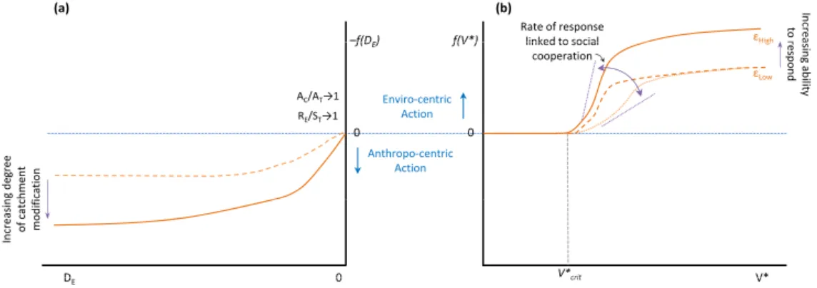
Theχ response function that determines the overall im-petus for action is designed to have a positive value to indi-cate a stimulus towards more enviro-centric measures, and a negative value to denote a drive towards more anthropocen-tric measures. In the simplest sense this can be composed as (Fig. 5)
χ=f V∗−f (DE) , (5)
whereV∗is a normalised sensitivity metric developed below.
As a general premise, decreasing sensitivity levels would be expected to be associated with higher annual rates of water extraction, land clearing and dam building, to a point, while the converse is expected to hold true for increases in sen-sitivity levels. The sensen-sitivity–response link has been made in the literature previously (Leichenko and O’Brien, 2002) and is broadly consistent with what has been observed in the development trajectories of river basins outlined earlier. Al-though this deals with the direction of an expected shift in the
χ function, a number of further hypotheses are put forward in terms of the timing and magnitude of such shifts. Firstly, it is believed that upward (i.e. positive) movements will be observably more “sticky” and demonstrate a greater time lag in response when compared with downward (i.e. negative) movements inχ, as the former seeks to “reverse” behaviour. Secondly, it is expected that a catchment’s baseline sensitiv-ity levels will affect the magnitude and timing of manage-ment action. For instance, catchmanage-ments operating at generally higher levels of the sensitivity scale (e.g. arid rural catch-ments) that experience an increase in sensitivity level over a period might be expected to show a more immediate and severe management response, relative to catchments operat-ing at the lower end of the sensitivity scale experiencoperat-ing the same absolute increase in sensitivity level. Finally, it is ex-pected that there will be points at both ends of the sensitivity scale beyond which there will be no observable change in management action.
(a)
εHigh
(b) Incre
a
to
r
Rate of response
linked to social ƒ(V*)
–ƒ(DE)
RE/ST→1
AC/AT→1 Enviro‐centric Action
High
εLow
a
sing
ability
respond
linked to social
cooperation ƒ(V )
ƒ(DE)
0 E/T
0
Anthropo‐centric Action
g
degree
hment
cation
V* V*crit
D 0
Increasin
of
catc
modifi
V crit
DE 0
Figure 5.A hypothetical illustration of how the Behavioural Response functions vary according to:(a)the change in catchment demand for
expansion,DE, and;(b)the change in collective community sensitivity,V∗. The functions can be customised according to factors such as
community cooperation or technological capability for enacting modifications to the catchment as indicated by the different lines.
modelled here as f V∗=
0 for V∗ ≤Vcrit∗
χmaxV
(V∗)σ
kVσ+(V∗)σ
f (ε) for V∗ > Vcrit∗ , (6a) whereχis proposed to follow a sigmoidal response function based onV∗, calculated at timetas
V∗= 1V
Vmax−Vt
, (6b)
where Vmax is an arbitrary constant reflecting the maxi-mum sensitivity of the particular community, and the term
Vmax−Vt scales the incremental change in sensitivity to in-creaseχas the baseline sensitivity approaches the maximum. In Eq. (6a),σ is a co-operativity function used to modify the rate at which χ will change (Schwarz and Ernst, 2009). It is intended to be related to the degree to which the commu-nity will collectively respond to a change in sensitivity levels, and can be calculated based on the defector fraction within the community,ω, or other relevant proxy, such as the per-centage of the catchment population holding memberships in social organisations. The termf (ε)captures the propensity for action based upon the national capacity to act in terms of financial and technological resources (based on the country’s level of development, whereby ε=EcN
EcS such that it reflects
the national rate of development beyond a baseline subsis-tence economy).
The second driver of theχ function can be thought of as the degree of inducement for agricultural expansion (DE). It is composed of two primary driving components (population growth and the relative importance and growth of agriculture in the economy) which may act independently or in tandem, limiting variables relating to the available land and water re-sources, and a moderating variable reflecting efficiency im-provements in resource utilisation. Such an approach is sim-ilar to that found by Barbier (2004) to adequately reflect the rate of land-use change in favour of agriculture in developing economies. The population will thus be motivated to change their interaction with the catchment land surface and water
balance in response to the demand for agricultural develop-ment as follows:
f (DE)=χmaxD
DE
(kD+DE)
, (7a)
where the Monod equation above is proposed to reflect the response function based onDE. This is calculated at timet
as
DE=
1P
n
Pt n
+f (ZC)
1−AC AT
1−RE ST
f (ζ ) , (7b)
where 1Pn
Pt
n is the population growth rate (similar to
Bar-bier’s (2004) rural population growth rate) andf (ZC)is a function of structural driving variables that could comprise agricultural export share, growth in agricultural value added, and/or agricultural crop yield (Barbier, 2004). The extent of development is mitigated by the extent of “capacity usage” of underlying natural resources within the catchment, namely land (AC/AT)and water (RE/ST)resources. The capacity us-age factor is included as manus-agement decisions are progres-sively less likely to acquiesce to expansion pressures as usage levels approach the capacity (i.e. land limited,AC/AT→1; or water limited,RE/ST→1). The variableζ is a composite efficiency metric that captures the improvement in existing land and water utilisation as a result of implementing effi-ciency measures (e.g. rainwater harvesting or agricultural in-tensification through the application of more efficient farm-ing technologies). It therefore acts to mediate demand for the underlying resources by enabling a degree of expansion that is not reliant on further resource exploitation. This term is thus driving humans to more actively modify the catchment water balance in favour of development, and will slow down as opportunities for further development reduce.
annual change in storage capacity. Each of the management response equations would then take the form, for example, of
dRE
dt =ηREfRE(χ ) (8a)
dAC
dt =ηACfAC(χ ) (8b)
dSmax
dt =ηSmaxfSmax(χ ) , (8c)
which then each feed into the hydrology model. In the above equations,ηis the translation factor that captures the extent to whichχmanifests in this particular water management ac-tion. The closure relationships used in Eq. (8) will be highly specific to any given context, thus each of these must be de-fined upon local catchment conditions, and are therefore left for practitioners to determine on a case-by-case basis. By way of example,fAC(χ )in Eq. (8b) might be parameterised as fAC(χ )=χafor case study site A, whereas it may take the form fAC(χ )= 2χ1/bfor case study site B, due to the distinctness of circumstances and response patterns between the sites.
4 The conceptual framework in practice
To demonstrate how the generic conceptual framework can be applied to analysing the evolution of different catchments, two agricultural catchments located in Australia have been selected for further illustration: the Murrumbidgee catch-ment in New South Wales and the Toolibin catchcatch-ment in Western Australia. The case studies have been chosen for illustration purposes based on differences in size and wa-ter balance drivers in each agricultural catchment. The Mur-rumbidgee catchment is examined as a large-scale irrigated river basin catchment, whilst the Lake Toolibin catchment provides a contrasting small-scale rainfed lake catchment. In light of these differences, case-study-specific manifestations of the generic conceptual framework are made possible, and tailored application of the model to unique catchment his-tories can be explored. Prior to full implementation of the model for these case studies, this paper outlines the approach to parameterisation of the above framework, and in particular the necessary closure relationships described above in gen-eral terms. Table 1 summarises how the differences between these two catchments are to be captured through application of the conceptual framework and how parameterisation of the closure relationships could be pursued. A stylised model that incorporates several of the above components of the frame-work is run for a 110-year timescale (1900–2010) for each catchment using various simplifying assumptions and some generic parameterisations to demonstrate the approach to ap-plication of the model.
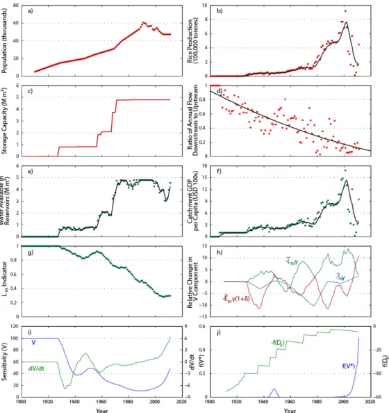
4.1 Murrumbidgee catchment
The trajectory of the Murrumbidgee catchment, an area of 8.4 million hectares located within the greater Murray– Darling River basin in southern New South Wales, has been described in detail by Kandasamy et al. (2014). The nation’s capital city, Canberra, is located within the catchment, along with numerous other regional towns and inland cities. The Murrumbidgee River, at 1600 km long, supports a diverse range of fish and bird species, along with numerous seasonal wetlands, nature reserves and riparian vegetation. The catch-ment is predominantly used for grazing and irrigated crop farming. The advent of increasingly extensive environmental problems in recent decades, including the adverse impacts of nutrient runoff and salinisation, has prompted concerted re-medial efforts at local, regional and state levels. It therefore presents a compelling case study for the implementation of the socio-hydrology framework on a large-scale area.
In addition to the extensive clearing of native vegetation to make way for agricultural expansion, humans vastly altered natural flow regimes throughout the catchment as a conse-quence of the large-scale development of dams and weirs for irrigation farming, which occurred up to 1970 (Kandasamy et al., 2014). A number of environmental problems began to appear in the latter half of the 20th century, and became progressively more serious. The considerable reallocation of water to irrigation led to the first major environmental crisis facing the sustained health of riverine and wetland ecosys-tems, with the diversion of up to 90 % of the Murrumbidgee river’s natural flow to irrigation causing a sharp decline in residual flows to the environment (Kandasamy et al., 2014). Marked reductions were recorded in water bird and native fish populations in the Murrumbidgee basin as a result.
The second major issue to arise pertained to the exces-sive discharge of nutrients from sewage treatment plants and farming practices into the Murray River, causing a sharp de-cline in water quality and threatening riverine ecosystems. In fact, one of the worst blue-green algal blooms anywhere on record occurred along more than 1000 km of the Murray– Darling rivers in the summer of 1991–1992. Furthermore, the widespread replacement of deep-rooted native vegeta-tion with shallow-rooted agricultural crops caused a rise in groundwater tables throughout the catchment, thereby dis-solving salts stored in the soil profile and transporting them to the surface. This led to the third key issue – land salinisa-tion – which threatened agricultural productivity, local liveli-hoods and the useful life of existing infrastructure, as well as having detrimental impacts on riverine ecology. This predica-ment was exacerbated by the use of irrigation, which created pervasive waterlogging (Kandasamy et al., 2014).