Abstract— In this work, the electrical signals obtained by
application of microwaves in chemical and bone tissues are analyzed and classified using techniques of signal processing and pattern recognition. For this, Wavelet Transform is applied as a method to extract relevant features of signal and KNN is used as a classification technique. The results showed that microwave signals can be analyzed using Wavelet Transform, which can be used to reconstruct the signals with minimal error rate and KNN showed satisfactory results.
Index Terms— Bone tissue, Microstrip antennas, Statistical pattern recognition, Wavelet transform.
I. INTRODUCTION
The increase in life expectancy of humans has awaking the interest of researchers for illnesses that
may arise as a result of this high estimate. Among these diseases stands Osteoporosis. The World
Health Organization (WHO) defines Osteoporosis as a disease characterized by deterioration of bone
tissue with the reduction of low bone density [1]. It is a condition that affects more women than men
because they have a less dense bone mass and an earlier bone loss [2]. In Brazil, Osteoporosis affects
approximately five million people. It is estimated that among women over 50 years, one in four
suffers from this problem. With respect to men, one in eight have developed the disease [3].
Several methods have been used to characterize and classify patterns obtained from medical signals
such as Wavelet, Fractal Theory, Statistical Methods, Fuzzy Theory, Artificial Neural Networks
(ANN), among others [5]. This paper presents an analysis and classification system of bone tissue and
bone meal using microwaves. To do this, Wavelet Transform was applied as a method to extract
features able to reconstruct the signals with minimum error and KNN was applied as a method to
classify the bone tissue in two groups: tissue with normal mass and tissue with reduced mass.
Characterization of Bone Tissue by
Microwaves Using Wavelets and KNN
Jannayna Domingues Barros1, José Josemar de Oliveira Júnior2, Sandro Gonçalves da Silva1, Robson Fernandes de Farias3
1
Programa de Pós Graduação em Engenharia Elétrica e Computação – UFRN
2
Escola de Ciências e Tecnologia – UFRN
3
Departamento de Química – UFRN
Campus Universitário, 59072-970, Natal-RN, Brazil
II. BONE TISSUE
The human body is divided into four types of tissue: connective tissue, nervous tissue, epithelial
tissue and muscle tissue. Connective tissues of the adult body are divided into proper connective
tissues and specialized connective tissues. Bone tissue is a specialized connective tissue characterized
by vascularization and hard consistency. It is the main tissue of mature bones. The hardness of bone
tissue is due to the large amount of mineral salts and collagen fibers in extracellular matrix. This
tissue is composed by three types of cell: osteoblasts, osteoclasts and osteocytes [2].
Our skeleton is made up of two hundred and six bones, divided in two types: cortical (compact) and
trabecular (spongy). Approximately 80% of all bone mass in skeleton is composed by cortical bone
and 20% of trabecular bone [3]. Figure 1 illustrates the difference between cortical and trabecular
bones.
Fig. 1. Types of Bones: 1 - Cortical, 2 - Trabecular [1].
The term osteoporosis was used for the first time in the nineteenth century in France and Germany
to describe the histological findings of bones in an elderly human, emphasizing the apparent porosity
[2]. Figure 2 presents a comparison between a normal bone and a bone with the disease.
Fig.2. A - Bone more dense and compact, considered normal; B – Spongy bone and less dense, characteristic of bones with Osteoporosis [2].
Osteoporosis affects more women than men because men have bones with more density and less
prone to fractures [2]. In literature, there is no evidence that isolated bone loss causes symptoms, so
that Osteoporosis is called "silent epidemic" [3]. Because of that, first clinical manifestations of
Osteoporosis are noticeable after 30% to 40% of bone mass loss. There is no consensus about the
other hand the diagnosis based on bone density allows the recognition of the disease at an early stage.
Osteoporosis can be considered a public health problem. The costs with treatment, diagnosis and
fractures rehabilitation are very high. A solution to this problem would be the use of methods to
diagnose the disease in its early stages, to prevent loss bone and to avoid fractures.
III. WAVELETS IN SIGNAL PROCESSING
Wavelet Transform is defined as one nonlinear operation used in analysis of non-stationary signals
in order to extract relevant information related to variations in frequency and time domains. This dual
location, combined with efficient algorithms to analysis and synthesis, allows the application of
wavelet in different areas [5].
Wavelets are widely used in characterization of signals in Digital Signal Processing (DSP) area
[5]. The initial researches on Wavelet Transform had the goal of creating basis functions that could be
used to describe mathematical functions or to analyze signals. Another aim was related to
multiresolution analysis, defined as one technique originated in signal processing area, to analyze
signals in multiple frequency bands [5]. In context of wavelets, multiresolution analysis is one
standard way to generate basis functions and models to wavelet transform in computer [7].
Wavelet Transform applied to continuous signal is calculated by Equation 1:
,
( , )
( )
j k( )
F a b
=
∫
f t
ψ
t dt
(1)where j and k represent the scaling and translation factors, respectively.
The function called wavelet is derived from a mother function . The combination of
scaling and translation properties applied to mother function generates daughter wavelet functions by
changing j and k. The wavelet term refers to all functions in the form of small waves created by
scaling and translation applied to one mother wavelet given by Equation 2:
, 0
1
( ) ; 0
j k
t k
t j
j j
ψ
=ψ
− ≠ (2)
where j and k, as mentioned previously, are the scaling and translation factors, respectively.
The daughter wavelets are generated by:
0 1 ( ) j t t scaling j j
ψ
=ψ
→ (3)
(
)
0
( )
k
t
t
k
translation
ψ
=
ψ
−
→
(4)Where is a constant of energy normalization, defined to each daughter wavelet. This term is
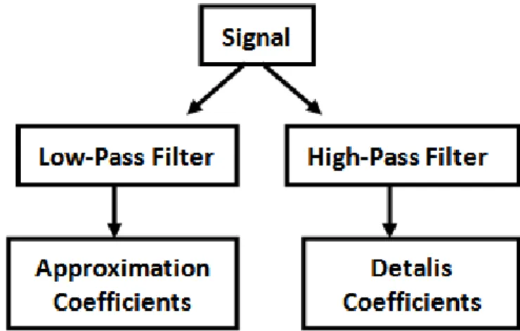
The wavelet transform could be implemented in an efficient way using the multiresolution
technique developed by Mallat [7]. This technique can be compared as the combination of high-pass
and low-pass filters, in which the function is related to high-pass filter, which produces the wavelet
coefficients of details, and other function, denominated scaling function, is related to low-pass
filter which produces the wavelet coefficients of approximation [5], as illustrated in Figure 3.
The main functions known as mother wavelets are Daubechies, Haar, Morlet and Meyer [7].
Fig. 3. Process of signal decomposition using multiresolution analysis.
In biomedical area, the wavelets analysis constituted an important tool with applicability in
different fields of medicine. In Maia [4], Wavelet Transform is used in the process of speech
recognition and signals compression. Two procedures were analyzed to evaluate wavelet performance
in these contexts: in the first, the signal was acquired and split in two sub-series and only one was
used in compression task. The second procedure consisted of acquiring, analyzing and comparing
signals with a words database. In signal processing several wavelets families were used: Haar,
Daubechies and Symlet. The results were considered satisfactory with Symlet 1, where compression
and word recognition rates stayed around 90%.
In Ferreira [8], the wavelets are used to extract and select features from mammograms in order to
identify the occurrence of cancer. The experiments were developed with two wavelets families: Haar
and Daubechies 4. Results showed that Haar wavelet was more accurate to classify images than
Daubechies. Application of wavelet in image classification was also presented in Soares [6]. This
work applied the wavelet analysis at images of skin cancer in different scales, to extract features such
as color, shape and texture. The Daubechies wavelet presented the best results.
In Orthopedic Medicine, studies using wavelet transform are also found. Krug et al. [9] applied
wavelets to characterize trabecular bone. The wavelets were used in images and the results were
compared with MRI analysis, which proved effectiveness of wavelet in image processing, because it
In Xu [10], wavelet analysis was used in ultrasound to bone characterization. This work
investigates analysis of ultrasonic signals using time-frequency techniques to determine density and
bone strength. Measurements were performed on three samples of human vertebral trabecular bones
using a transducer at frequency of 1 MHz. The data were processed using Mallat algorithm. The
obtained wavelet representation is compared to one similar obtained from a reference signal. The
time-frequency relationship was calculated and the results indicate that this ratio could be used to
discriminate several biophysical states.
In this work, wavelets are used to extract relevant features that could be used to reconstruct
electromagnetic signals with minimum error. These signals were obtained from non-ionizing radiation
using microwave applied to bone tissue and bone meal.
IV. KNN – K NEAREST NEIGHBORS
The techniques of pattern recognition based on statisticals are used in the design of commercial
systems for recognition. These techniques can be applied in different areas, such as data mining,
multimedia data retrieval, face recognition, word recognition and other applications that require
efficient and robust techniques [14]. In Pattern Recognition with statistical approaches, each pattern is
represented in terms of features and could be seen as a point in d-dimensional space. The
classification is based on concepts of statistical decision theory that defines the boundaries of decision
between classes of patterns based on probability distribution.
Although there are different approaches to classification, all have the same goal: minimize the
classification errors and reduce the computational cost. A classifier is considered ideal when it obtains
a high accuracy rate with speed and efficiency. K-Nearest Neighbors (KNN) is one kind of statistical
classifier chosen in this work because it has simple implementation and good results. It creates
complex boundaries from a set of training patterns with known classes. Thus, given a certain
unknown pattern x, its class is calculated by the distance between x and the other training patterns.
The unknown pattern is compared with the k closest patterns to x and it is associated to class more
often between the k patterns. To calculate this distance, we use the Euclidean distance or other
measure.
This classifier builds a decision rule directly without estimating the conditional probability
densities, providing a simple and efficient method, widely used in practice [15]. The main advantage
of KNN is the creation of an adaptive boundary decision to training data distribution. This
characteristic allows obtaining good recognition rates [14]. Among the limitations of this classifier,
we highlighted that the number of neighbors (k) is considered a critical point and there is no analytical
solution for this. We recommended the application of trial and error strategy to its definition. Another
limitations are related to problems of indecision when occurs a tie, and the high computational cost
due to the high number of operations needed to classify a pattern because it considers the attribute
V. METHODOLOGY
This article uses wavelet transform to extract relevant features in order to reconstruct the original
signal with precision and KNN is used to classify the signals into two categories: bone tissue with
normal mass and bone tissue with reduced mass. For feature extraction, we used three types of
wavelets known in the literature [5]: Daubechies 6, Daubechies 7 and Symlet 4. For each signal, it
was decomposed into 3, 6 and 9 levels in order to determine the wavelet family and level of
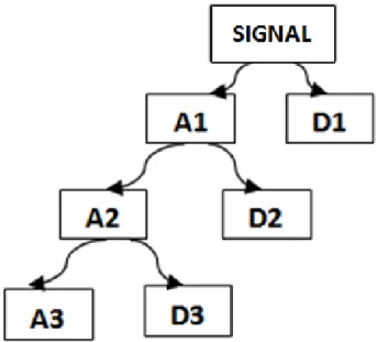
decomposition with the best result in the reconstruction process. Figure 4 illustrates a tree of wavelet
decomposition in three levels, the approximation coefficients are decomposed three times in other
coefficients of approximation and details, increasing the resolution of signal analyzed.
Fig. 4. Wavelet decomposition tree with three levels of approximation and details coefficients.
For classification stage, we use KNN assigning three values for k: k = 1, k = 3 and k = 5. The
classifier was applied on the coefficients from wavelet Daubechies 6 and Symlet 4. The experiments
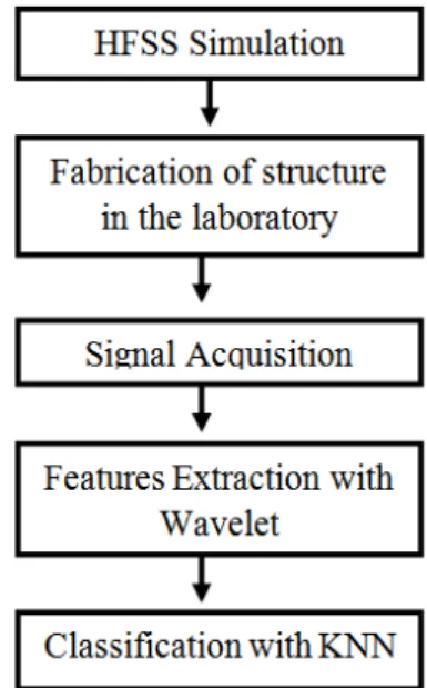
Fig. 5. Block diagram used in bone tissue characterization.
Initially, the antennas were designed using commercial software (Ansoft HFSS® [11]) with the
goal of verify the behavior of these antennas at the frequency range desired. Figure 6 presented the
Smith Chart with information about impedance matching and Figure 7 shows the return loss. These
results were extracted from HFSS. The projected antennas show a good impedance matching for the
resonance frequency (2.44 GHz). The maximum resonance point occurs in 2.41 GHz with attenuation
of -20 dB that can be considered one good value of attenuation [12].
5.00 2.00 1.00 0.50 0.20 5.00 -5.00 2.00 -2.00 1.00 -1.00 0.50 -0.50 0.20 -0.20 0.00 -0.00 0 10 20 30 40 50 60 70 80 90 100 110 120 130 140 150 160 170 180 -170 -160 -150 -140 -130 -120 -110
-100 -90 -80 -70 -60 -50 -40 -30 -20 -10
Ansoft Corporation Smith Plot 1 HFSSDesign1
m1 m 2
Curve Info
S(LumpPort1,LumpPort1) Setup1 : Sw eep1
Name Freq Ang Mag RX
m1 2.4000 6.8323 0.1171 1.2625 + 0.0357i
m2 2.4100 64.7638 0.0980 1.0695 + 0.1915i
2.00 2.20 2.40 2.60 2.80 3.00 Freq [GHz] -25.00 -20.00 -15.00 -10.00 -5.00 0.00 d B (S (L u m p P o rt 1 ,L u m p P o rt 1 ))
nsoft Corporation XY Plot 1 HFSSDesign1
m1 m2
Curve Info dB(S(LumpPort1,LumpPort1)) Setup1 : Sw eep1
Name X Y
m1 2.4100 -20.1748
m2 2.4000 -18.6295
Fig.7. Return loss of microstrip antenna simulated in HFSS.
Then, the antennas were manufactured in laboratory. The structure proposed to the patch has
rectangular geometry, with one resonance frequency of 2.44 GHz, fed by a microstrip line with an
effective length of 3.09 cm. This frequency is allocated in the frequency range released by Anatel
(Brazilian FCC) for Medical, Industrial and Scientific Applications. The antenna construction was
made using the substrate of fiberglass or FR4 with permittivity of 4.4. Fig. 8 illustrates the antennas
used to acquire the signals. In sequence, the antennas were measured on Network Analyzer (HP
8714C model).
Fig.8. Microstrip antennas manufactured in laboratory.
The experiments were conducted using two types of materials: five samples of bone meal
compound with silica and six bovine femora. Non-ionizing radiation were applied to both material at
the same frequency range from 2.0 to 2.8 GHz. Initially, the experiments were performed in bone
be used to determine variations in the level of attenuation accordingly to different amounts of bone
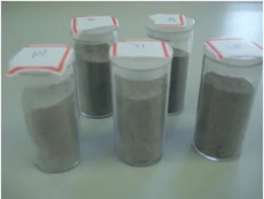
meal. For this, we used five samples with different quantities of bone meal and silica. Figure 9
illustrates the samples used.
Fig.9. Samples of bone meal compound with silica.
Table I shows the quantities of bone meal and silica to each sample.
TABLE I.QUANTITIES OF BONE MEAL AND SILICA TO EACH SAMPLE
Sample Bone Meal (mL) Silica(mL)
1 25 5
2 20 10
3 15 15
4 10 20
5 5 25
The bone meal was purchased in specialized shops and it presents high levels of Calcium (Ca) and
Phosphorus (P). The chemical compound silicon dioxide, also known as Silica, is an oxide of silicon
with the chemical formula of SiO2. The silica can be found in crystalline form, as in quartz, topaz and
amethyst, and amorphous form, as silica gel or colloidal silica [13]. In this work, the silica gel was
used in experiments. The silica gel is an inorganic polymer composed by siloxane groups (Si-O-Si)
inside and silanol groups (Si-OH) on its surface [7].
The samples were placed in acrylic cylinders with a diameter of 3.0 cm and 6.0 cm tall. The acrylic
was chosen because it is "transparent" to radiation in range used at the study, so any variation observed
can be attributed solely to sample.
The second part of experiments was performed using six bovine femora. In some cases, the
experiments on animals can be the best option, since animal model reproduces satisfactorily aspects of
the disease in humans. This fact is used at the work because bovine bone has one high similarity with
Fig.10. Bovine bones used in experiment.
VI. RESULTS
A. Bone meal and silica
The samples were submitted to radiation and the electromagnetic signals were analyzed to verify
their attenuation. The results obtained for samples 2, 3 and 4 present similar behaviors at frequency
range from 2.4 to 2.5 GHz, but in samples 1 and 5, which have the biggest variation in the proportion
of silica and bone meal, occur a variation of 0.6 dB in attenuation. Figure 11 shows the attenuation
obtained.
After that, wavelet transform has been applied to extract features of such signals, for this, Matlab
software was used in both processes of decomposition through filters and reconstruction of signals.
The reconstruction was done by generating an approximation of the original signal using the
coefficients obtained in decomposition. For each sample analyzed one curve of attenuation and three
Fig.11. Attenuation versus frequency obtained in different samples of bone meal and silica in the range of 2400 and 2500 MHz.
The number of coefficients generated by wavelet decomposition at 3, 6 and 9 levels is presented in
Table II.
TABLE II. NUMBER OF COEFFICIENTS GENERATED BY WAVELET DECOMPOSITION
Wavelet 3 levels 6 levels 9 levels
Daubechies 6 56 88 121
Daubechies 7 63 101 140
Symlet 4 45 65 86
Tables III, IV and V shows the reconstruction errors of each signal, decomposed in 3, 6 and 9
TABLE III. WAVELET WITH 3 LEVELS OF DECOMPOSITION
Samples Daubechies 6 Daubechies 7 Symlet 4
1 1.88e-11 1.70e-11 2.38e-12
2 1.24e-11 1.30e-11 2.66e-12
3 1.72e-11 1.56e-11 2.22e-12
4 1.13e-11 1.22e-11 2.85e-12
5 1.46e-11 1.46e-11 2.77e-12
TABLE IV. WAVELET WITH 6 LEVELS OF DECOMPOSITION
Samples Daubechies 6 Daubechies 7 Symlet 4
1 6.56e-11 7.44e-11 2.17e-11
2 6.21e-11 6.46e-11 1.39e-11
3 6.09e-11 7.25e-11 2.00e-11
4 6.68e-11 6.53e-11 1.14e-11
5 5.10e-11 5.83e-11 1.51e-11
TABLE V. WAVELET WITH 9 LEVELS OF DECOMPOSITION
Samples Daubechies 6 Daubechies 7 Symlet 4
1 1.52e-10 1.38e-10 3.56e-11
2 1.12e-10 1.31e-10 3.47e-11
3 1.22e-10 1.31e-10 3.51e-11
4 1.05e-10 1.37e-10 3.78e-11
5 1.10e-10 1.13e-10 2.96e-11
Analyzing the tables, we conclude that wavelet Symlet 4 with three levels of decomposition
obtained the best result, because the signals were reconstructed with the lowest error.
B. Bovine Bone
The signals obtained from bovine bone were submitted to the same procedure described above.
Initially, the bones with normal mass were subjected to microwave radiation. In these cases was
verified that the maximum attenuation occurred in range of 2.4 GHz to 2.5 GHz, varying between -30
and -40 dB. After that, the samples were drilled for reduce their bone mass. Table VI shows the bone
mass before and after drilling for each sample.
TABLE VI.BONEMASSBEFOREANDAFTERDRILLING
Bone Initial mass (g) Mass after drilling (g)
1 246 169
2 260 151
3 265 198
4 274 141
5 309 237
6 270 207
It can be observed that the attenuation to these samples with bone mass reduced have the highest
attenuation in range of 2.5 to 2.6 GHz, varying between -10 and -20 dB. Figure 12 illustrates the
Fig.12. Attenuation versus frequency obtained in different samples of bovine bones in range of 2400 to 2600 MHz. In blue solid line, the attenuations of samples with normal mass. In red circles, the attenuations of samples with reduced mass.
Tables VII, VIII and IX present the results obtained with Wavelet decomposition.
TABLE VII. WAVELET WITH 3 LEVELS OF DECOMPOSITION
Samples Daubechies 6 Daubechies 7 Symlet 4
1 5.85e-11 8.54e-11 2.15e-11
2 2.31e-11 3.43e-11 7.87e-12
3 2.23e-11 1.77e-11 1.18e-12
4 7.26e-11 9.08e-11 2.08e-11
5 4.09e-11 3.63e-11 4.91e-11
6 4.00e-11 6.29e-11 1.65e-11
TABLE VIII. WAVELET WITH 6 LEVELS OF DECOMPOSITION
Samples Daubechies 6 Daubechies 7 Symlet 4
1 8.81e-11 1.51e-10 4.64e-11
2 5.65e-11 8.07e-11 2.35e-11
3 5.72e-11 5.47e-11 1.44e-11
4 9.47e-11 1.56e-10 4.99e-11
5 7.49e-11 7.91e-11 2.49e-11
6 8.57e-11 1.33e-10 3.94e-11
TABLE IX. WAVELET WITH 9 LEVELS OF DECOMPOSITION
Samples Daubechies 6 Daubechies 7 Symlet 4
1 9.01e-11 1.50e-10 5.09e-11
2 7.39e-11 9.41e-11 2.65e-11
3 8.15e-11 7.18e-11 1.68e-11
4 9.46e-11 1.51e-10 5.47e-11
5 1.01e-11 9.28e-11 2.69e-11
6 1.08e-10 1.50e-10 4.35e-11
smallest reconstruction error when compared to other wavelet families. Figure 13 exemplifies the
decomposition and reconstruction of one signal using wavelet.
Fig.13. Example of the signal decomposition and reconstruction using the wavelet.
After extraction of wavelet coefficients, signals were subjected to the process of pattern
recognition using KNN. For this, we used the wavelet coefficients from Daubechies 6 and Symlet 4,
both with three levels of decomposition. These coefficients were applied in KNN for signals obtained
in two frequency bands: 2.4 to 2.5 GHz (frequency range released by Anatel (Brazilian FCC) for
Medical, Industrial and Scientific Applications) and 2.4 to 2.6 GHz, being the range which occurs the
biggest attenuation for both groups. Tables X and XI show the results for k = 1, k = 3 and k = 5.
TABLE X.RECOGNITIONRATEOBTAINEDUSINGDAUBECHIES6TODIFFERENTVALUESOFK
Frequency (GHz) K=1 K=3 K=5
2.4 – 2.5 70.83% 66.66% 62.5% 2.4 – 2.6 45.83% 54.16% 54.16%
TABLE XI.RECOGNITIONRATEOBTAINEDUSINGSYMLET4TODIFFERENTVALUESOFK
Frequency (GHz) K=1 K=3 K=5
2.4 – 2.5 54.16% 58.33% 58.33% 2.4 – 2.6 58.33% 62.5% 58.33%
With these results, we conclude that the best accuracy rate was obtained with Daubechies 6 in
frequency range of 2.4 to 2.5 GHz using k = 1. The increase in value of k in this frequency range
decreases the recognition rate. The outcome was different in frequency range of 2.4 to 2.6 GHz
because in this case the best recognition rate was obtained using Symlet 4 and k = 3, although this rate
VII. CONCLUSION
In this study, we conclude that microwaves are able to identify variations in bone density based on
different levels of attenuation observed in the analyzed samples. The Wavelet Transform was applied
to electromagnetic signals and it can be used to extract relevant features of these signals and their
coefficients can be used to represent it in a compact form. These signals were obtained from
experiments with bone meal mixed with silica and bovine bones. The results of decomposition and
reconstruction using wavelet shown Symlet 4 presents the smallest error in all experiments. KNN was
a good method for classification of signals. In classification, the best result was obtained using KNN
with k = 1 and wavelet coefficients of Daubechies 6 family with 70.83% of accuracy rate. Future
work will apply the wavelet coefficients in a bone mass classification system using Artificial Neural
Networks.
ACKNOWLEDGMENT
TO UFRN AND CNPQ FOR THE FINANCIAL SUPPORT OF THIS WORK.
REFERENCES
[1] De POLLI, Yasmara Conceição. Caracterização da Anisotropia na Permissividade de Osso Cortical Utilizando o Método da Impedância. USP - São Paulo, 2008.
[2] SZEJNFELD, Vera Lúcia. Osteoporose: Diagnóstico e Tratamento. São Paulo: Sarvier, 2000.
[3] GALI, Julio Cesar. Atualização em Osteoporose. Revista da Faculdade de Ciência Médicas, Sorocaba - SP, v.4; n.1-2; p.1-5, 2002. [4] MAIA, Joaquim Miguel. Sistema Ultra-Sônico para Auxílio ao Diagnóstico da Osteoporose. Master Thesis. UNICAMP – Campinas, 2001.
[5] OLIVEIRA, Hélio Magalhães. Análise de Sinais para Engenheiros – Uma abordagem via Wavelets. Rio de Janeiro: Brasport, 2007. [6] SOARES, Heliana Bezerra. Análise e Classificação de Imagens de Lesões da Pele por Atributo de Cor, Forma e Textura utilizando Máquina de Vetor de Suporte. PhD Thesis. UFRN – RN, 2008.
[7] SILVA, A. V.; EYNG, J. Wavelets e Wavelet Packets. UFSC,2000.
[8] FERREIRA, C. R.; BORGES, D. L. Uma Estratégia de Seleção de Subconjunto Mínimo de Características Wavelets em uma Abordagem Multirresolução para Classificação de Tumores em Mamogramas. IV SQBS – V Workshop de Informática Médica. Porto Alegre, RS, 2005.
[9] KRUG, R. et al. Wavelet Based Characterization of Vertebral Trabecular Bone Structure from MR Images of Specimen at 3 Tesla Compared to MicroCT Measurements. Engineering in Medicine and Biology 27th Annual Conference. Pages 7040-7043, vol. 1, Shanghai, China, 2005.
[10] XU, W. et al. Applications of Wavelet Analysis to Ultrasonic Characterization of Bone. Signals, Systems and Computers. Pages 1090 – 1094, vol. 2, Pacific Grove, CA, 1994.
[11] MRABET, O. High Frequency Structure Simulator (HFSS) – Tutorial. France, 2006. [12] VOLAKIS, J. L. Antenna Engineering Handbook. 4th Edition: McGraw-Hill Companies, 2007.
[13] AIROLDI, C.; FARIAS, R. F.. O Uso de Sílica Gel Organofuncionalizada como Agente Sequestrante para Metais. Química Nova, Vol. 23, No.4, São Paulo, 2000.
![Fig. 1. Types of Bones: 1 - Cortical, 2 - Trabecular [1].](https://thumb-eu.123doks.com/thumbv2/123dok_br/18887555.424184/2.892.259.648.417.656/fig-types-bones-cortical-trabecular.webp)