HESSD
8, 11171–11232, 2011Amazon discharge simulation using ORCHIDEE forced by
new datasets
M. Guimberteau et al.
Title Page
Abstract Introduction
Conclusions References
Tables Figures
◭ ◮
◭ ◮
Back Close
Full Screen / Esc
Printer-friendly Version
Interactive Discussion
Discussion
P
a
per
|
Dis
cussion
P
a
per
|
Discussion
P
a
per
|
Discussio
n
P
a
per
Hydrol. Earth Syst. Sci. Discuss., 8, 11171–11232, 2011 www.hydrol-earth-syst-sci-discuss.net/8/11171/2011/ doi:10.5194/hessd-8-11171-2011
© Author(s) 2011. CC Attribution 3.0 License.
Hydrology and Earth System Sciences Discussions
This discussion paper is/has been under review for the journal Hydrology and Earth System Sciences (HESS). Please refer to the corresponding final paper in HESS if available.
Discharge simulation in the sub-basins of
the Amazon using ORCHIDEE forced by
new datasets
M. Guimberteau1,2, G. Drapeau1,2,3,4, J. Ronchail1,2,3, B. Sultan1,2,5, J. Polcher2,6, J.-M. Martinez7, C. Prigent8, J.-L. Guyot7, G. Cochonneau7, J. C. Espinoza9,10, N. Filizola11, P. Fraizy12, W. Lavado10,13, E. De Oliveira14, R. Pombosa15, L. Noriega16, and P. Vauchel12
1
Laboratoire d’Oc ´eanographie et du Climat: exp ´erimentations et approches num ´eriques (LOCEAN), UMR7159, Paris, France
2
Institut Pierre Simon Laplace (IPSL), France
3
Universit ´e Paris Diderot, Sorbonne Paris Cit ´e, France
4
P ˆole de Recherche pour l’Organisation et la Diffusion de l’Information G ´eographique (PRODIG), Paris, France
5
Institut de Recherche pour le D ´eveloppement (IRD), France
6
Laboratoire de M ´et ´eorologie Dynamique (LMD), CNRS, Paris, France
7
HESSD
8, 11171–11232, 2011Amazon discharge simulation using ORCHIDEE forced by
new datasets
M. Guimberteau et al.
Title Page
Abstract Introduction
Conclusions References
Tables Figures
◭ ◮
◭ ◮
Back Close
Full Screen / Esc
Printer-friendly Version
Interactive Discussion
Discussion
P
a
per
|
Dis
cussion
P
a
per
|
Discussion
P
a
per
|
Discussio
n
P
a
per
|
8
Laboratoire d’Etudes du Rayonnement et de la Mati `ere en Astrophysique (LERMA), Observatoire de Paris, CNRS, Paris, France
9
Instituto Geofisico del Per ´u (IGP), Lima, Per ´u
10
Universidad Agraria La Molina (UNALM), Lima, Per ´u
11
Universidad Federal do Amazonas (UFAM), Manaus, Brazil
12
Institut de Recherche pour le D ´eveloppement (IRD), Lima, Per ´u
13
Servicio Nacional de Meteorolog´ıa e Hidrolog´ıa (SENAMHI), Lima, Per ´u
14
Ag ˆencia Nacional de ´Aguas (ANA), Brasilia, Brazil
15
Instituto Nacional de Meteorolog´ıa e Hidrolog´ıa (INAMHI), Quito, Ecuador
16
Servicio Nacional de Meteorolog´ıa e Hidrolog´ıa, La Paz, Bolivia
HESSD
8, 11171–11232, 2011Amazon discharge simulation using ORCHIDEE forced by
new datasets
M. Guimberteau et al.
Title Page
Abstract Introduction
Conclusions References
Tables Figures
◭ ◮
◭ ◮
Back Close
Full Screen / Esc
Printer-friendly Version
Interactive Discussion
Discussion
P
a
per
|
Dis
cussion
P
a
per
|
Discussion
P
a
per
|
Discussio
n
P
a
per
Abstract
The aim of this study is to evaluate the ability of the ORCHIDEE land surface model to simulate streamflows over each sub-basin of the Amazon River basin. For this purpose, simulations are performed with a routing module including the influence of floodplains and swamps on river discharge and validated against on-site hydrological
measure-5
ments collected within the HYBAM observatory over the 1980–2000 period. When forced by the NCC global meteorological dataset, the initial version of ORCHIDEE shows discrepancies with HYBAM measurements with underestimation by 15 % of the annual mean streamflow at ´Obidos hydrological station. Consequently, several im-provements are incrementally added to the initial simulation in order to reduce those
10
discrepancies. First, values of NCC precipitation are substituted by HYBAM daily situ rainfall observations from the meteorological services of Amazonian countries, in-terpolated over the basin. It highly improves the simulated streamflow over the northern and western parts of the basin, whereas streamflow over southern regions becomes overestimated, probably due to the extension of rainy spots that may be exaggerated
15
by our interpolation method, or to an underestimation of simulated evapotranspiration when compared to flux tower measurements. Second, the initial map of maximal frac-tions of floodplains and swamps which largely underestimates floodplains areas over the main stem of the Amazon River and over the region of Llanos de Moxos in Bo-livia, is substituted by a new one with a better agreement with different estimates over
20
the basin. Simulated monthly water height is consequently better represented in OR-CHIDEE when compared to Topex/Poseidon measurements over the main stem of the Amazon. Finally, a calibration of the time constant of the floodplain reservoir is per-formed to adjust the mean simulated seasonal peak flow at ´Obidos in agreement with the observations.
HESSD
8, 11171–11232, 2011Amazon discharge simulation using ORCHIDEE forced by
new datasets
M. Guimberteau et al.
Title Page
Abstract Introduction
Conclusions References
Tables Figures
◭ ◮
◭ ◮
Back Close
Full Screen / Esc
Printer-friendly Version
Interactive Discussion
Discussion
P
a
per
|
Dis
cussion
P
a
per
|
Discussion
P
a
per
|
Discussio
n
P
a
per
|
1 Introduction
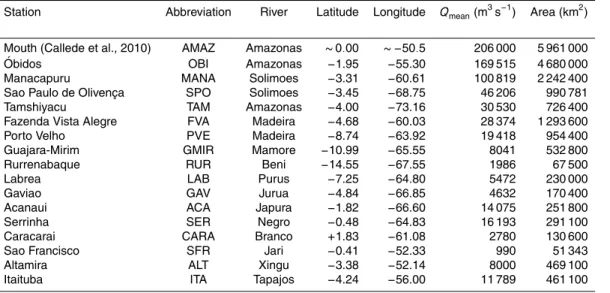
The Amazon River basin, the largest basin in the world with an area of approximately 6.0 million km2, has the highest average discharge (206 000 m3s−1) (Callede et al., 2010) and it contributes to about 15–20 % of the fresh water transported to the oceans (Richey et al., 1986). The present functioning of this basin is especially complex due
5
to four elements: its expansion over large ranges of latitude, longitude and altitude that organize its mean hydrological characteristics, the presence of extensive inunda-tion zones that contribute to runoff control at annual and interannual time scale, the influence of the Atlantic and Pacific oceans that partly control the hydrological vari-ability at different time scales, and the land use changes that are increasing since
10
the seventies and drive modification in the radiative and hydrological balances of the basin. Yet, a good understanding of the present hydrological response of the Amazon River basin to various forcings is required to evaluate future changes. This can be partly achieved by using numerical models relying on hydroclimatological databases. So far, regional discharge simulation in the Amazon River basin has been conducted
15
by different groups. V ¨or ¨osmarty et al. (1989) and Costa and Foley (1997) initiated the simulation efforts in the Amazon River basin. Coe et al. (2002) simulated discharge in 121 stations of the Amazon River basin using an integrated biosphere simulator cou-pled to a hydrological routing algorithm and obtained good results for Brazilian basins. However, a discharge underestimation was found in the basins pertaining to other
Ama-20
zonian countries, due to the lack of reliable rainfall information except for Brazil. Other deficiencies of the model, related to the river and floodplain morphology, have been corrected in Coe et al. (2007) and allowed a great improvement of the simulation of discharge, water height and flooded area. In Coe et al. (2009), the same authors used the model to characterize the role of deforestation on runoffevolution. Also using ISBA
25
HESSD
8, 11171–11232, 2011Amazon discharge simulation using ORCHIDEE forced by
new datasets
M. Guimberteau et al.
Title Page
Abstract Introduction
Conclusions References
Tables Figures
◭ ◮
◭ ◮
Back Close
Full Screen / Esc
Printer-friendly Version
Interactive Discussion
Discussion
P
a
per
|
Dis
cussion
P
a
per
|
Discussion
P
a
per
|
Discussio
n
P
a
per
river discharge observations. At the beginning of the 20th century, a distributed Large Basin Simulation Model, called MGB-IPH (an acronym from the Portuguese for Large Basins Model and Institute of Hydraulic Research), was developed by Collischonn and Tucci (2001). Applications of this model were initially developed for the La Plata basin (Allasia et al., 2006) and then for some Amazonian rivers, the Madeira (Ribeiro et al.,
5
2005), the Tapajos, where satellite-derived rainfall information is being used to run the model (Collischonn et al., 2008), and the Negro river, where spatial altimetry data is being used to complement the validation of the simulation (Getirana, 2010; Getirana et al., 2010). The comparison of different rainfall products used to force MGB-IPH in the Negro basin shows that observed data give the most adequate discharge results
10
(Getirana et al., 2011). Recently, developments towards a better representation of floodplains in the upper Parana River (Pantanal region) have been presented in Paz et al. (2010). Beighley et al. (2009) focused on the representation of water storage in the Amazon River basin and the factors accounting for its variability. Finally, Paiva et al. (2011) show that it is possible to employ full hydrodynamic models within
large-15
scale hydrological models even using limited data for river geometry and floodplain characterization.
This present work aims to evaluate the simulation of discharge in the Amazon main stem and in its principal tributaries by the hydrological module SECHIBA (Sch ´ematisation des EChanges Hydriques `a l’Interface Biosph `ere-Atmosph `ere,
20
Ducoudr ´e et al., 1993) of the land surface model (LSM) ORCHIDEE (ORganising Car-bon and Hydrology In Dynamic EcosystEms) considering a 11-level hydrology (De Ros-nay, 1999; De Rosnay et al., 2002; d’Orgeval, 2006; d’Orgeval et al., 2008), using a routing module (Polcher, 2003) and the representation of floodplains and swamps by d’Orgeval (2006). All these characteristics of the model are described in Sect. 2.
25
HESSD
8, 11171–11232, 2011Amazon discharge simulation using ORCHIDEE forced by
new datasets
M. Guimberteau et al.
Title Page
Abstract Introduction
Conclusions References
Tables Figures
◭ ◮
◭ ◮
Back Close
Full Screen / Esc
Printer-friendly Version
Interactive Discussion
Discussion
P
a
per
|
Dis
cussion
P
a
per
|
Discussion
P
a
per
|
Discussio
n
P
a
per
|
simulations forced by this new 53-yr NCC data is better than the former ones forced by the GSWP2 (Global Soil Wetness Project 2, Dirmeyer et al., 2002; Zhao and Dirmeyer, 2003) forcing dataset. However, the discharge simulations forced by NCC pointed out some discrepancies in the annual cycles in some tributaries of the Amazon River basin and over- or underestimations of the mean discharge in the southern and western
5
tributaries, respectively (Ronchail et al., personal communication). Improvements to former simulations may be expected thanks to the recent availability of a comprehen-sive observed precipitation dataset for the Amazon River basin made available within the framework of the ORE (Environmental Research Observatory) HYBAM (Geody-namical, hydrological and biogeochemical control of erosion/alteration and material
10
transport in the Amazon River basin, Cochonneau et al., 2006) and of new satellite-derived maps of floodplains and swamps distribution (Martinez and Le Toan, 2007; Prigent et al., 2007). These new data datasets are described in Sect. 3.3. Our aim is to verify whether ORCHIDEE, forced by these new datasets, properly reproduces the different specificities of the main stem and of some large sub-basins of the
Ama-15
zon when compared with observations (described in Sect. 3.2). Therefore, the new datasets are incrementally added to the initial simulation (ORCH1) performed with NCC and initial maps of flooded areas distribution. First, in simulation ORCH2, we test in Sect. 4 the impact of HYBAM precipitation on simulated water budget (Sect. 4.1) and simulated streamflow (Sect. 4.2) over the basin. The different characteristics of the
20
simulated discharges (accuracy of the mean annual value, precision of the seasonal cycle and representation of the interannual variability) are studied in the different loca-tions of the basin. Finally, the impact of the new spatial distribution of flooded areas on the time position of flooding and the water height of the floodplains is investigated through simulation ORCH3 in Sect. 5. Those improvements allowed us to calibrate the
25
HESSD
8, 11171–11232, 2011Amazon discharge simulation using ORCHIDEE forced by
new datasets
M. Guimberteau et al.
Title Page
Abstract Introduction
Conclusions References
Tables Figures
◭ ◮
◭ ◮
Back Close
Full Screen / Esc
Printer-friendly Version
Interactive Discussion
Discussion
P
a
per
|
Dis
cussion
P
a
per
|
Discussion
P
a
per
|
Discussio
n
P
a
per
by Callede et al. (2004) and Marengo (2004) but may be also a consequence of the climatic change described for South America by the IPCC (Solomon et al., 2007).
2 The land surface model ORCHIDEE
2.1 Hydrological module and vegetation
SECHIBA is the hydrological module of ORCHIDEE that simulates the fluxes between
5
the soil and the atmosphere through the vegetation, and computes runoffand drainage, which are both discharged to the ocean. The hydrological module used in this study is based on developments by De Rosnay et al. (2000, 2002) and d’Orgeval (2006). Physical processes of vertical soil flow are represented by a diffusion-type equation resolved on a fine vertical discretization (11 levels) and the partitioning between surface
10
infiltration and runoff is represented in the model. The hydrological module is fully described by De Rosnay (1999); De Rosnay et al. (2002); d’Orgeval (2006); d’Orgeval et al. (2008).
In order to reduce noise in our simulation of streamflow, no complex scenario such as deforestation, land use or forest fire are taken into account in this study.
Vegeta-15
tion distribution and LAI seasonality are prescribed in the model through global maps. In each grid-cell, up to thirteen Plant Functional Types (PFTs) can be represented si-multaneously according to the International Geosphere Biosphere Programme (IGBP, Belward et al., 1999) and the Olson classification (Olson et al., 1983). Values of LAI come from the Normalized Difference Vegetation Index (NDVI) observations (Belward
20
HESSD
8, 11171–11232, 2011Amazon discharge simulation using ORCHIDEE forced by
new datasets
M. Guimberteau et al.
Title Page
Abstract Introduction
Conclusions References
Tables Figures
◭ ◮
◭ ◮
Back Close
Full Screen / Esc
Printer-friendly Version
Interactive Discussion
Discussion
P
a
per
|
Dis
cussion
P
a
per
|
Discussion
P
a
per
|
Discussio
n
P
a
per
|
2.2 Routing module
The routing scheme (Polcher, 2003), described in Ngo-Duc et al. (2007), is activated in the model in order to carry the water from runoffand drainage simulated by SECHIBA to the ocean through reservoirs, with some delay. The routing scheme is based on a parametrization of the water flow on a global scale (Miller et al., 1994; Hagemann
5
and Dumenil, 1998). Given the global map of the main watersheds (Oki et al., 1999; Fekete et al., 1999; V ¨or ¨osmarty et al., 2000) which delineates the boundaries of sub-basins and gives the eight possible directions of water flow within the pixel, the surface runoffand the deep drainage are routed to the ocean. The resolution of the basin map is 0.5◦, higher than usual resolution used when LSMs are applied. Therefore, we can
10
have more than one basin in SECHIBA grid cell (sub-basins) and the water can flow either to the next sub-basin within the same grid cell or to the neighboring cell. In each sub-basin, the water is routed through a cascade of three linear reservoirs which do not interact with the atmosphere. The water balance within each reservoir is computed using the following continuity equation:
15
dVi
dt =Q
in
i −Q
out
i (1)
whereVi (kg) is the water amount in the reservoiri considered (i=1, 2 or 3),Q
in
i and
Qouti (both in kg day−1) are, respectively the total inflow and outflow of the reservoiri.
The slow and deep reservoir (i =3) collects the deep drainage D (water moving downward from surface water to groundwater) computed by the land surface scheme,
20
HESSD
8, 11171–11232, 2011Amazon discharge simulation using ORCHIDEE forced by
new datasets
M. Guimberteau et al.
Title Page
Abstract Introduction
Conclusions References
Tables Figures
◭ ◮
◭ ◮
Back Close
Full Screen / Esc
Printer-friendly Version
Interactive Discussion
Discussion
P
a
per
|
Dis
cussion
P
a
per
|
Discussion
P
a
per
|
Discussio
n
P
a
per
can be written for each of the three reservoirs as below: dV1
dt =
X
x
Qinx−Qout1 (2)
dV2
dt =R−Q
out
2 (3)
dV3
dt =D−Q
out
3 (4)
whereQxin(kg day−
1
) is the total inflow coming from the neighboring cells or sub-basins
5
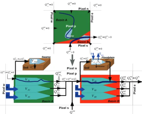
xandR andD(both in kg day−1) are, respectively surface runoffand deep drainage. The flow chart in Fig. 1 represents the routing channel modeling in SECHIBA through an example of two sub-basins (A and B) included in a same grid cell p. Three reservoirs are allocated to each sub-basins. At each routing time step ∆t=1 day, the routing scheme computes water flows as follows: the sum of the surface runoffand the deep
10
drainage is spread in the grid cell p over the two sub-basins, proportionally to their surface. The surface runoffof the sub-basins A and B (respectivelyRAp andRBp) flows
into their respective fast reservoirs of volumeVA2andVB2. The deep drainageDAp and
DB
p flows into the slow reservoirs of volume VA3 and VB3. The water amount of the
river is represented by the stream reservoir. The stream reservoir of the sub-basin A is
15
assumed to be empty in this example (VA1=0), the outflows from the neighboring pixels
x(x=sw,w,nw,n,ne) to sub-basin A being null (P
xQ
out
x =0). The stream reservoir of
the downstream sub-basin B of volumeVB1 collects the sum of the outflowsQ out Ap from
the three reservoirs of the sub-basin A (see Eq. 5) and the outflowQouts coming from the pixel s (Eq. 6).
20
QoutA p =
3
X
i=1
QoutAi
HESSD
8, 11171–11232, 2011Amazon discharge simulation using ORCHIDEE forced by
new datasets
M. Guimberteau et al.
Title Page
Abstract Introduction
Conclusions References
Tables Figures
◭ ◮
◭ ◮
Back Close
Full Screen / Esc
Printer-friendly Version
Interactive Discussion
Discussion
P
a
per
|
Dis
cussion
P
a
per
|
Discussion
P
a
per
|
Discussio
n
P
a
per
|
whereQoutA
p (kg day
−1
) is the total outflow from the sub-basin A in the pixel p andQoutAi p
(kg day−1) the outflow from each reservoiri of the sub-basin A in the pixel p.
QinB p=Q
out Ap +Q
out
s (6)
where QinB
p (kg day
−1
) is the total inflow of the sub-basin B in the pixel p and Qouts
(kg day−1) the total outflow from the pixel s.
5
The sum of the outflows from the reservoirs of the sub-basin B in the pixel p goes to the pixel e. Runoffand drainage are routed through this cascade of reservoirs. In our model, the volume of waterVi into the reservoir i is assumed to be linearly related to its outflowQouti :
Vi=(gi·k)·Qouti (7)
10
wheregi (day m−
1
) is a property of the reservoiri andk (m) a water retention index. The water travel simulated by the routing scheme is dependent on a water retention indexk, given by a 0.5◦ resolution map for each pixel performed from a simplification
of Manning’s formula (Dingman, 1994; Ducharne et al., 2003):
k= s
d3
∆z (8)
15
whered (m) is the river length from one subgrid basin to the next subgrid, and∆z (m) the height lost over the path of the river.
The value of g in the Eq. (7) has been calibrated for the three reservoirs over the Senegal river basin only, during the 1◦ NCC resolution simulations (Ngo-Duc et al., 2005; Ngo-Duc, 2006) and generalized for all the basins of the world. The “slow
reser-20
voir” and the “fast reservoir” have the highest value (g2=g3=3.0 days m− 1
) in order to simulate the groundwater. The “stream reservoir”, which represents all the water of the stream, has the lowest value (g1=0.24 day m−
1
HESSD
8, 11171–11232, 2011Amazon discharge simulation using ORCHIDEE forced by
new datasets
M. Guimberteau et al.
Title Page
Abstract Introduction
Conclusions References
Tables Figures
◭ ◮
◭ ◮
Back Close
Full Screen / Esc
Printer-friendly Version
Interactive Discussion
Discussion
P
a
per
|
Dis
cussion
P
a
per
|
Discussion
P
a
per
|
Discussio
n
P
a
per
basins of the world. The resulting productgi·k represents the time constantTi (day)
which is an e-folding time, the time necessary for the water amount in the stream reser-voir to decrease by a factor e. Hence, it gives an order of magnitude of the travel time through this reservoir between the sub-basin considered and its downstream neighbor.
2.3 Floodplains and swamps module
5
Floodplains are land areas adjacent to streams that are subject to recurring inundation. The stream overflows its banks onto adjacent lands. Moreover, water can be stored in swamps, it saturates and infiltrates into the soil and does not return to the river. These inundated areas mainly correspond to flooded forest areas in the Amazon River basin. Thus, the module of floodplains/swamps developed in ORCHIDEE by d’Orgeval (2006)
10
is used for this study in order to better represent the timing of flow in some regions of the Amazon River basin strongly affected by inundations. The parametrization is described in detail by d’Orgeval (2006); d’Orgeval et al. (2008). A map of maximal fractions of floodplains (MFF) and swamps (MFS) derived from the Global Lakes and Wetlands Database (GLWD, Lehner and D ¨oll, 2004) is initially prescribed to the model.
15
Floodplains and swamps in the model derive, respectively from three types of water surfaces (Reservoir, Freshwater marsh-Floodplain and Pan-Brackish/Saline wetland) and one type (Swamp forest-Flooded forest) according to GLWD database.
Over floodplains areas, the streamflowQinB
pfrom head waters of the reservoirs of the
basin A flows into a reservoir of floodplains (QinB p=Q
in
Fd) instead of the stream
reser-20
voir of volumeVB1 of the next downstream (Fig. 1). The surface SFd of the floodplain
depends on the shape of the bottom of the floodplain in order to simulate the timing between the rise of water level and its expansion. Finally, water from the floodplains reservoir that has not evaporated or reinfiltrated the soil flows into the stream reservoir of volume VB1 of the basin B after a delay. This delay is characterized by the time
HESSD
8, 11171–11232, 2011Amazon discharge simulation using ORCHIDEE forced by
new datasets
M. Guimberteau et al.
Title Page
Abstract Introduction
Conclusions References
Tables Figures
◭ ◮
◭ ◮
Back Close
Full Screen / Esc
Printer-friendly Version
Interactive Discussion
Discussion
P
a
per
|
Dis
cussion
P
a
per
|
Discussion
P
a
per
|
Discussio
n
P
a
per
|
constantTFd(day) function of the surface of the floodplainsSFd:
TFd=gFd·SFd SB
(9)
wheregFd=4.0 days is a property of the floodplain reservoir, SFd (m2) the surface of the floodplain andSB (m
2
) the surface of the basin.
The value ofgFd has been calibrated through observations in the Niger Inner Delta
5
and can thus be different for the Amazon River basin as it will be shown in Sect. 5.1. Over swamp areas, a fraction of waterα=0.2 is uptaken from the stream reservoir of volumeVA1(Q
in
Swp=αQ in
Ap). It is transferred into soil moisture (Fig. 1) and thus does not
return directly to the river. The swamp storage enhances transpiration of forest where the soil is saturated, reducing bare soil evaporation.
10
3 Datasets
In this section, the datasets used in this work are presented: the atmospheric forcing, the validation data and the new rainfall and flooded areas distribution datasets used to force ORCHIDEE.
3.1 Atmospheric forcing
15
The atmospheric data set used as input to ORCHIDEE is NCC (NCEP/NCAR Cor-rected by CRU data, Ngo-Duc et al., 2005) based on the NCEP/NCAR reanalysis project (Kistler et al., 2001) and in-situ observations. The spatial resolution is 1◦
×1◦
for the whole globe. The temporal resolution is six hours and the time series cover the 1948–2000 period. All variables present in the forcing are summarized in Table 1.
20
HESSD
8, 11171–11232, 2011Amazon discharge simulation using ORCHIDEE forced by
new datasets
M. Guimberteau et al.
Title Page
Abstract Introduction
Conclusions References
Tables Figures
◭ ◮
◭ ◮
Back Close
Full Screen / Esc
Printer-friendly Version
Interactive Discussion
Discussion
P
a
per
|
Dis
cussion
P
a
per
|
Discussion
P
a
per
|
Discussio
n
P
a
per
of the reanalysis product. The data has allowed to simulate the 50-yr river flows over the planet (Ngo-Duc et al., 2005).
3.2 Data of validation
3.2.1 ORE HYBAM gauge stations
Discharge data has been gathered and complemented within the frame of the ORE
5
(Environmental Research Observatory) HYBAM (Geodynamical, hydrological and bio-geochemical control of erosion/alteration and material transport in the Amazon River basin – http://www.ore-hybam.org/), a partnership which associates the meteorologi-cal and hydrologimeteorologi-cal services of the Amazonian countries (Ag ´encia Nacional de ´Aguas Water National Office/ANA in Brazil (http://www2.ana.gov.br/), Servicio Nacional de
10
Meteorolog´ıa e Hidrolog´ıa/National Meteorology and Hydrology Service/SENAMHI in Peru (http://www.senamhi.gob.pe/) and Bolivia (http://www.senamhi.gob.bo/), Instituto Nacional de Meteorolog´ıa e Hidrolog´ıa / National Meteorology and Hydrology Insti-tute/INAMHI in Ecuador (http://www.inamhi.gov.ec/)) and the French Institute of Re-search for Development (IRD – http://www.ird.fr/). The rating curves have been
de-15
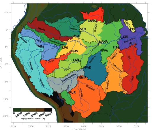
termined using the stream gauging measurements, recently with Acoustic Doppler Current Profiler (ADCP), and have been used to convert the water level series into discharge data. The daily water level data was corrected when necessary, eventually complemented using its correlation with data of upstream or downstream stations. Six-teen stations out of eighty were chosen to realize the comparison with simulated data
20
(Fig. 2 and Table 2). The choice of these stations depended on:
– the length of the records. Those beginning in the late seventies were preferred to the others in order to get longer common series with the simulated data. How-ever, in order to have information about most sub-basins, some short series were retained in places where no other record exists.
HESSD
8, 11171–11232, 2011Amazon discharge simulation using ORCHIDEE forced by
new datasets
M. Guimberteau et al.
Title Page
Abstract Introduction
Conclusions References
Tables Figures
◭ ◮
◭ ◮
Back Close
Full Screen / Esc
Printer-friendly Version
Interactive Discussion
Discussion
P
a
per
|
Dis
cussion
P
a
per
|
Discussion
P
a
per
|
Discussio
n
P
a
per
|
– the proximity of the stations. A choice was made between close stations as a func-tion of the reliability of the records (absence of lacking value).
– the size of the river. Some very small rivers were not recognizable with OR-CHIDEE due to the coarse resolution.
3.2.2 Topex/poseidon measurements
5
Surface monitoring by satellite altimetry has been performed on the whole Earth since 1993 (Cr ´etaux et al., 2011). Altimetry datasets are available over the main stem of the Amazon and the Rio Negro-Branco rivers for a time period common to ours (1993– 2000) thanks to Topex/Poseidon satellite mission. These measurements are used to assess the accuracy of ORCHIDEE to simulate floodplain height variability.
10
3.3 New basis of observations over the Amazon River basin
In order to simulate the streamflow with higher accuracy over the Amazon River basin, a new set of observations of precipitation is used to force ORCHIDEE and validate NCC. A new map of MFF and MFS based on observations is also tested and com-pared with the initial map prescribed to the model. The details of the construction and
15
implementation of these new datasets are described in this section.
3.3.1 HYBAM precipitation
Global rainfall datasets usually rely on very sparse in-situ observations over the Ama-zon River basin. Consequently, the AmaAma-zonian precipitation is often poorly represented in such datasets, especially regarding the plain of the Andean countries (Espinoza
20
HESSD
8, 11171–11232, 2011Amazon discharge simulation using ORCHIDEE forced by
new datasets
M. Guimberteau et al.
Title Page
Abstract Introduction
Conclusions References
Tables Figures
◭ ◮
◭ ◮
Back Close
Full Screen / Esc
Printer-friendly Version
Interactive Discussion
Discussion
P
a
per
|
Dis
cussion
P
a
per
|
Discussion
P
a
per
|
Discussio
n
P
a
per
retained with data covering more than five-year continuous periods, and the lowest probability of errors in their series. Because a few extremely rainy spots located on the foothills of the Eastern Andes bring large amounts of water to the western and south-western parts of the basin (Killeen et al., 2007), we then chose to replace miss-ing values of these particular stations by estimated values usmiss-ing linear regressions or
5
by long-term climatological means. A strong underestimation of the rainfall input is thus avoided for the periods when records of one or several of these wet spots are missing. The concerned locations are the Chapare region in Bolivia (Cristal Mayu and Misicuni stations), the Manu-Tambopata area (Quincemil and San Gaban stations) and the Selva Central region (Tingo Maria station) in Peru. In-situ observations were
after-10
ward spatially interpolated to the resolution of NCC (1◦
×1◦). Geostatistics have been
widely used to interpolate environmental variables such as rainfall (Goovaerts, 2000; Hevesi et al., 1992). Ordinary kriging has notably been shown to provide better es-timates than conventional methods, as it takes into account the spatial dependence between neighbouring observations, which is expressed by a semi-variogram. In this
15
study, ordinary kriging was thus performed to generate an observation-based gridded daily rainfall dataset. Finally, because other NCC variables were available at a 6-h tem-poral resolution, daily rainfall grids were segmented at this resolution following a diurnal cycle as described in NCC precipitation data. If the NCC precipitation is null for the four 6 h time-steps in the day, the HYBAM daily value is spread equally over the time-steps.
20
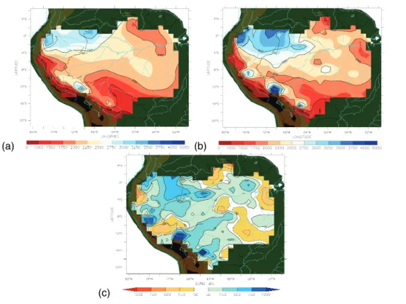
Mean annual value of NCC precipitation over the basin is about 2044 mm yr−1 whereas HYBAM precipitation shows a higher value than NCC (2190 mm yr−1 i.e. +7.1 %). The mean annual spatial distribution in precipitation is shown over the Ama-zon River basin for both datasets in Fig. 3a,b and their difference is calculated (Fig. 3c). In both datasets, the spatial distribution of precipitation of the Amazon River basin is
25
quite similar. The rainiest regions (3000 mm yr−1 and more) are located in the
HESSD
8, 11171–11232, 2011Amazon discharge simulation using ORCHIDEE forced by
new datasets
M. Guimberteau et al.
Title Page
Abstract Introduction
Conclusions References
Tables Figures
◭ ◮
◭ ◮
Back Close
Full Screen / Esc
Printer-friendly Version
Interactive Discussion
Discussion
P
a
per
|
Dis
cussion
P
a
per
|
Discussion
P
a
per
|
Discussio
n
P
a
per
|
Northwest of the Amazon to the Subtropical South Atlantic (Vera et al., 2006). Rainfall decreases toward the tropics, reaching less than 1500 mm yr−1in the Peruvian-Bolivian plain and toward the north in the Roraima Brazilian state. Rainfall also diminishes with altitude: in the Andes, over 2000 m, annual rainfalls lower than 1000 mm are the most frequent. However, some differences in precipitation rate exist between the two
5
datasets. HYBAM depicts a sharp increase by 250 to 750 mm yr−1 of the amount of rainfall in the north-west of the basin toward the southern and eastern part of this area. Extremely high values can be measured in the wet spots of the Eastern Andes foothills, in positions that favor strong air uplift; in these very rainy spots scattered along the Cordillera, annual rainfall reaches 5000 to 6000 mm with HYBAM (regions of
Chu-10
ruyacu in Colombia, of the Reventador Volcano in Ecuador, of San Gab ´an and Tingo Maria in Peru, of the Chapar ´e in Bolivia) whereas these spots of precipitation are much less significant in NCC dataset. Finally, drier regions are present in HYBAM compared to NCC over the south-east of the basin, the region of the Amazon mouth, the extreme north of the basin and over Ecuador and Central Peru.
15
3.3.2 Map of maximal fractions of floodplains and swamps
Initially, the maps of MFF and MFS prescribed to ORCHIDEE were derived from the GLWD dataset of Lehner and D ¨oll (2004) (hereafter called “GLWD”). In this study, a new map (hereafter called “PRIMA”) is produced where MFF and MFS are, respec-tively derived from Prigent et al. (2007) and Martinez and Le Toan (2007) dataset at
20
0.25◦
×0.25◦ and interpolated at 0.5◦×0.5◦ for ORCHIDEE. Prigent et al. (2007)
es-timated monthly inundated fractions over the world by multisatellite method for eight years (1993–2000). Then, for each 0.5◦ pixel of the Amazon River basin, as we need it for ORCHIDEE, we determine the maximal value that has been recorded during the 8 yr observation. As there is no distinction between floodplains and swamps in
Pri-25
HESSD
8, 11171–11232, 2011Amazon discharge simulation using ORCHIDEE forced by
new datasets
M. Guimberteau et al.
Title Page
Abstract Introduction
Conclusions References
Tables Figures
◭ ◮
◭ ◮
Back Close
Full Screen / Esc
Printer-friendly Version
Interactive Discussion
Discussion
P
a
per
|
Dis
cussion
P
a
per
|
Discussion
P
a
per
|
Discussio
n
P
a
per
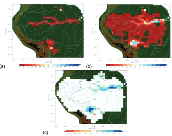
The GLWD and PRIMA maps are compared for floodplains (Fig. 4) and swamps (Fig. 5). For both water surfaces, the difference between the two maps is performed. For both datasets, floodplains are located along the main stem of the Solimoes-Amazon River, in the southern region of the basin in Llanos de Moxos and to a lesser extent along the Ireng river (in GLWD) or the Branco river (in PRIMA) in the
northern-5
most region of the basin (Fig. 4). However, MFF of PRIMA map are globally higher than GLWD (respectively about 4.2 and 2.6 % of the total area of the Amazon River basin according to Table 3). Moreover, in PRIMA map, many MFF lower than 5 % within the mesh cover almost all the basin whereas GLWD does not give data over these regions. The difference in MFF between the two maps is particularly high along the main stem
10
of the Solimoes-Amazon River and especially near the mouth (between+5 to+15 % before Manacapuru to more than +70 % around ´Obidos (see Fig. 2 and Table 2 for localization of the two stations)). We note that a small percentage of this difference (up to about 2 % around Obidos) is explained by the fact that Prigent et al. (2007)’s data take into account the surface of the river while Lehner and D ¨oll (2004) data does not.
15
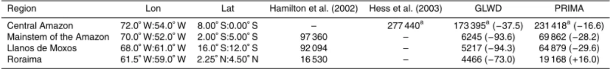
In the south, the region of Llanos de Moxos shows the same order of increase in MFF with PRIMA dataset particularly over the Mamor ´e river in Bolivia. In Llanos de Moxos and along the main stem of the Solimoes-Amazon River, PRIMA is in better agreement with Hamilton et al. (2002)’s estimates with an underestimation of MFF by 30 % which is much lower than GLWD (near 100 %) according to Table 4. In the North, at Roraima
20
region, PRIMA is again in better agreement with Hamilton et al. (2002)’s estimates (about+15 %) than GLWD (about−70 %). For MFS, PRIMA presents half the extent of
GLWD across the river basin (Table 3). According to Fig. 5c, this decrease is observed over the western part of the basin and mainly in the Northern Peruvian region (up to 45 % more over some pixels), the south-easternmost part of the basin and along the
25
HESSD
8, 11171–11232, 2011Amazon discharge simulation using ORCHIDEE forced by
new datasets
M. Guimberteau et al.
Title Page
Abstract Introduction
Conclusions References
Tables Figures
◭ ◮
◭ ◮
Back Close
Full Screen / Esc
Printer-friendly Version
Interactive Discussion
Discussion
P
a
per
|
Dis
cussion
P
a
per
|
Discussion
P
a
per
|
Discussio
n
P
a
per
|
To summarize, combining floodplains and swamps, the total maximal fractions in PRIMA are lower on average over the Amazon River basin when compared to GLWD (Table 3). Estimates over Central Amazon were performed by Hess et al. (2003) for the flood period May–August 1996 where water surfaces have been differentiated and classified. We sum the two classes “Non vegetated-flooded” and “Non woody-flooded”
5
for comparison with our “Floodplains” class and “Woody-flooded” class is considered to be equivalent to “Swamps”. On average over the Central Amazon, PRIMA shows an underestimation of less than by 20 % of total MFF and MFS compared to Hess et al. (2003)’s estimates whereas GLWD underestimation is near by 40 % (Table 4). Moreover, according to Hess et al. (2003), flooded forest (i.e. swamps) constituted
10
nearly 70 % of the entire wetland area during high water period in this region. The distribution of swamps according to PRIMA is close to this estimate with a value of 61 % whereas GLWD largely overestimates it (95 %). Fig. 6 shows a comparison in MFF and MFS between Hess et al. (2003)’s estimates, GLWD and PRIMA datasets in three points over the main stem of the Amazon River. MFF with GLWD is systematically
15
underestimated throughout the main stem whereas PRIMA is in better agreement with estimates even if MFF remains lower than the estimates by Hess et al. (2003). MFS in PRIMA is well distributed at Curuai (about 20 %) and Cabaliana (about 40 %) but for the western region of the main stem, GLWD gives much higher MFS (about 65 %) than PRIMA (about 35 %) in agreement with estimates (about 70 %).
20
4 Simulated water budget and streamflows over the basin: impact of NCC
precipitation corrected by HYBAM
4.1 Simulated water budget
The study of water budget led to many estimates from models, reanalysis and lately measurements of fluxes. A non-exhaustive list of the annual values from some
esti-25
HESSD
8, 11171–11232, 2011Amazon discharge simulation using ORCHIDEE forced by
new datasets
M. Guimberteau et al.
Title Page
Abstract Introduction
Conclusions References
Tables Figures
◭ ◮
◭ ◮
Back Close
Full Screen / Esc
Printer-friendly Version
Interactive Discussion
Discussion
P
a
per
|
Dis
cussion
P
a
per
|
Discussion
P
a
per
|
Discussio
n
P
a
per
Amazonia (LBA) measurements) is given in Table 5 in average over the Amazon River basin and in different regions of the basin. In comparison, results from simulations ORCH1 (ORCHIDEE forced by NCC) and ORCH2 (ORCHIDEE forced by NCC cor-rected by HYBAM precipitation) are shown. According to the different estimates, the water budget components over the whole basin are about 6.2±1.1 mm d−1 in precip-5
itationP, 3.9±0.7 mm d−1 in evapotranspiration (ET) and 2.99 mm d−1 in runoff (R).
We note that the uncertainty is high in the estimations inP andE (their standard de-viations are around 1.0 mm d−1). Runo
ff is estimated from one value from Callede et al. (2010)’s estimate with an error of 6 %. Moreover, according to Marengo (2006), the different estimates of areas of the Amazon River basin generate uncertainty in the
10
estimations of runoff at the mouth of the Amazon. Thus, an uncertainty also exists in comparison with simulated runoff. In the model, it is computed from a total sur-face of basin equal to 5 853 804 km2(Fekete et al., 1999) which is lower (−1.8 %) than
Callede et al. (2010)’s estimate (5 961 000 km2). Precipitation over the whole basin is about 5.6 mm d−1 according to NCC. It is underestimated when compared to the
av-15
erage value of the estimations. Furthermore, it is also lower than the median of the observations (5.9 mm d−1). NCC value is higher than GPCP estimate (5.2 mm d−1),
equal to CMAP but underestimated when compared to the five other estimates. HY-BAM data (6.0 mm d−1) is closer to the average value and the median of the esti-mations. It is equal to CRU average value and close to the estimates by Marengo
20
(2005) (5.8 mm d−1) and LW (5.9 mm d−1). Simulated ET over the whole basin (about 2.8 mm d−1) seems to be underestimated when compared to the average value given by Da Rocha et al. (2009). ET variation between the two simulations is not signifi-cant. ET is more limited by the amount of incident energy, which is the same in both simulations, rather than by precipitation change. The resulting simulated runoffat the
25
HESSD
8, 11171–11232, 2011Amazon discharge simulation using ORCHIDEE forced by
new datasets
M. Guimberteau et al.
Title Page
Abstract Introduction
Conclusions References
Tables Figures
◭ ◮
◭ ◮
Back Close
Full Screen / Esc
Printer-friendly Version
Interactive Discussion
Discussion
P
a
per
|
Dis
cussion
P
a
per
|
Discussion
P
a
per
|
Discussio
n
P
a
per
|
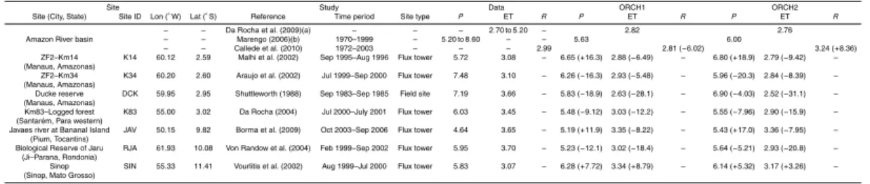
in the model. SimulatedP and ET are also compared with measurements (Table 5) from six LBA flux towers and one field site. They are located along the main stem of the Amazon River and over the south-eastern part of the basin (see Fig. 7 for the local-ization). The results confirm the underestimation in simulated ET for both simulations in the central region of the basin (K14, K34, DCK and K83) and in the south (RJA and
5
JAV). The underestimation at JAV is only 8 % but may be more sinceP in the model is high compared to observation (+12 to +17 %). Moreover, the low underestimation at JAV and the slight overestimation at SIN (+3 to 9 %) in ET compared to measure-ments occur in a region facing deforestation. However, in this region, the tropical forest covers 98 % of the grid cell area in the model, whereas the measurements have been
10
performed over a transitional tropical forest. Thus, as long as ORCHIDEE does not take into account deforestation, the comparison with observation in this region may be biased where simulated ET can be overestimated.
Regarding the underestimation in ET near Manaus, measurements of precipitation and ET are available for two years (September 1983–September 1985) (Shuttleworth,
15
1988). Moreover, evaporation over leaves (Ev) and transpiration (Tv) data are
distin-guished. Table 6 shows a comparison of the annual rate of these variables between the two simulations and observations. First, the results in precipitation show an un-derestimation in annual rate between observations and both simulations. However, underestimation is lower (−4 %) when NCC is corrected by HYBAM data. Moreover, 20
a better accuracy in variability is found compared to measurements (r2of ORCH1 and ORCH2 are, respectively 0.66 and 0.71). Both forcings give less precipitation than ob-served at the end of 1984 and particularly in December (Fig. 8a). Then, ORCH2 is in better agreement with measurements during the dry period. During the next wet pe-riod in 1985, the variability of precipitation is not well represented in both simulations.
25
HESSD
8, 11171–11232, 2011Amazon discharge simulation using ORCHIDEE forced by
new datasets
M. Guimberteau et al.
Title Page
Abstract Introduction
Conclusions References
Tables Figures
◭ ◮
◭ ◮
Back Close
Full Screen / Esc
Printer-friendly Version
Interactive Discussion
Discussion
P
a
per
|
Dis
cussion
P
a
per
|
Discussion
P
a
per
|
Discussio
n
P
a
per
the ratio between evaporation of water over the leaves (Ev) and transpiration (Tv). Vari-ation of Ev during the time period is improved in ORCH2 compared to ORCH1 (the
coefficients of correlation with observations are, respectively 0.6 and 0.7 with ORCH1 and ORCH2, Table 6) where a low seasonality was simulated throughout the period (Fig. 8b). Moreover,Ev overestimation observed with ORCH1 (+77 %) is reduced by
5
more than half (+27.5 %) on average over the period with ORCH2 (Table 6). As Ev
is reduced,Tv increases with ORCH2 but remains underestimated (respectively about
54 and 66 % for ORCH1 and ORCH2 according to Table 6) throughout the time pe-riod (Fig. 8c). However, the seasonal variation is in agreement with observations (r2
is, respectively 0.7 and 0.8 with ORCH1 and ORCH2 according to Table 6) where dry
10
season and wet season are well differentiated (Fig. 8c).
The precipitation over the Amazon River basin is improved by the use of HYBAM daily dataset. However, ET does not change between the two simulations and remains underestimated compared to observations. This discrepancy may be attributed to the low transpiration simulated by the model that has been pointed out at Manaus. In
15
ORCH2, the resulting simulated runoff at the mouth of the Amazon is consequently overestimated. In the next section, the annual simulated streamflow variation will be studied in the main sub-basins of the Amazon. Moreover, results in streamflow will be discussed when the observations of precipitation and floodplains/swamps distribution are implemented in the forcing of the model.
20
4.2 Simulated river discharge at ´Obidos and over the sub-basins of the Amazon
River
The mean annual streamflow estimated at the mouth of the Amazon River basin is about 206×103m3s−1(2.99 mm d−1) with an error of 6 % due to the method, for a total
area of 5 961 000 km2 and the time period 1972–2003 (Callede et al., 2010).
Sim-25
HESSD
8, 11171–11232, 2011Amazon discharge simulation using ORCHIDEE forced by
new datasets
M. Guimberteau et al.
Title Page
Abstract Introduction
Conclusions References
Tables Figures
◭ ◮
◭ ◮
Back Close
Full Screen / Esc
Printer-friendly Version
Interactive Discussion
Discussion
P
a
per
|
Dis
cussion
P
a
per
|
Discussion
P
a
per
|
Discussio
n
P
a
per
|
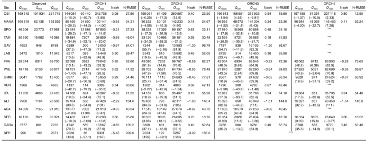
(191×103m3s−1) compared to Callede et al. (2010)’s estimates (−7.42 %) whereas
with ORCH2, an overestimation is found (220×103m3s−1i.e.+6.56 %). We note that
the differences in streamflow between simulation and observation are of the same or-der than the estimated error in observation. The increase of about 15 % in streamflow of the Amazon between ORCH1 and ORCH2 is mainly due to the increase in
precipita-5
tion (+6.75 %) (ET did not change) when NCC data is corrected by HYBAM. At the OBI station, which is the nearest gauged station from the outlet of the basin, mean annual simulated streamflow with ORCH1 is highly underestimated (−15 %) compared to
BAM discharge measurements, whereas with ORCH2 it is in good agreement with HY-BAM (−0.25 %) (Table A1). Thus, between OBI and the mouth of the Amazon, a large 10
quantity of water, overestimated in both simulations, comes from the south-eastern river basins (Xingu and Tapajos Rivers) as found at ITA (+20 %) and ALT (more than +90 %) according to Table A1 (see Fig. 2 and Table 2 for localization of the stations).
At OBI station, about 20 % of discharge comes from southern basins (FVA), 20 % from northern basins (ACA, SER, CARA), 30 % from western/south-western basins
15
(SPO, GAV, LAB) and 30 % from central residual basins (between SPO and MANA (hereafter called “MANA*”) and between MANA and OBI (hereafter called “OBI*”)) (Es-pinoza et al., 2009a) (see Fig. 2 and Table 2 for localization of the stations). With simulation ORCH1, the underestimation of streamflow at OBI is mainly due to the low streamflow over western/south-western regions of the basin (near−35 % at TAM) and 20
over the two central residual basins (between−25 to more than−35 %) (Fig. 9a). The
streamflow coming from the south is close to the observations but it is a compensation between the overestimation at RUR and GMIR and the underestimation over the two southern residual basins (hereafter called “PVE*” and “FVA*”). Simulated streamflow in northern stations like ACA and SER is close to the observations and an
overestima-25
tion is observed over the northernmost region of the basin at CARA. The correction of NCC precipitation by HYBAM data leads to a decrease of the error with observation over Andean sub-basins (−24 % at TAM) and over the residual basin of MANA* where
HESSD
8, 11171–11232, 2011Amazon discharge simulation using ORCHIDEE forced by
new datasets
M. Guimberteau et al.
Title Page
Abstract Introduction
Conclusions References
Tables Figures
◭ ◮
◭ ◮
Back Close
Full Screen / Esc
Printer-friendly Version
Interactive Discussion
Discussion
P
a
per
|
Dis
cussion
P
a
per
|
Discussion
P
a
per
|
Discussio
n
P
a
per
residual basin of OBI* is not improved. It can be due to the lack of available rainfall gauges for kriging over this region (see Fig. 1 of Espinoza et al., 2009b). The overes-timation of streamflow over all the southern sub-basins (except RUR) by 25 % to more than 35 %, mainly due to the increase of the rainy spots, leads to an excess of water at FVA. Consequently, simulated streamflow from ORCH2 at OBI station, close to the
ob-5
servations, is a result of a compensation between southern and western/south-western regions.
The observed streamflow at OBI has a pronounced seasonality during the year (Fig. 10a). It points out an average high-flow during May and June with a maximal value of about 230×103m3s−1. Then, a decrease occurs during five months until the 10
low-flow in November (near 103×103m3s−1). Simulated streamflow is time shifted in
both simulations compared to the observations (Fig. 10a). In fact, according to cross-correlation statistic (see Appendix for more details), cross-correlation between simulated and observed discharges would be optimal if a time lag of 1 month was applied (dt=1
andrcross=0.91,rcross=0.93 for ORCH1 and ORCH2, respectively). However, Nash
15
coefficient (see Appendix for more details) is increased when ORCHIDEE is forced by NCC precipitation corrected by HYBAM (0.08 and 0.40, respectively for ORCH1 and ORCH2 according to Table A1) indicating a significant improvement of the simulation in streamflow at OBI when HYBAM precipitation is used. The simulated interannual variation in streamflow is better captured with ORCH2 according to the coefficient of
20
variation of the root mean squared error (see Appendix for more details) which is lower (22.5 %) than with ORCH1 (28 %). The simulated low-flow is improved (−17 % with
ORCH2 compared to−41 % with ORCH1) but remains underestimated for most years
whereas simulated high-flow is slightly overestimated with ORCH2 (+5 %) even more during some dry years (1981, 1985, 1992) (Fig. 10b).
25
HESSD
8, 11171–11232, 2011Amazon discharge simulation using ORCHIDEE forced by
new datasets
M. Guimberteau et al.
Title Page
Abstract Introduction
Conclusions References
Tables Figures
◭ ◮
◭ ◮
Back Close
Full Screen / Esc
Printer-friendly Version
Interactive Discussion
Discussion
P
a
per
|
Dis
cussion
P
a
per
|
Discussion
P
a
per
|
Discussio
n
P
a
per
|
underestimated everywhere except in the north at ACA and SER. The improvement of the seasonal cycles at TAM and SPO is pointed out when precipitation is corrected by HYBAM data. The underestimation in low-flow is reduced by about 50 %. The Nash coefficient becomes positive in these stations, reaching 0.5. This mainly contributes to the increase in low flow at OBI with ORCH2 compared to ORCH1 and becomes
5
in better agreement with observations. Moreover, the increase in precipitation in the north-western part of the basin induces a better seasonality. At station ACA, no change in Nash coefficient is shown but at SER, the seasonality is well captured when com-pared to observations (Nash coefficient reaches about 0.80). Interannual variation of streamflow at this station is also well simulated as shown in Fig. 12 (N-RMSE for
10
ORCH1 and ORCH2 are, respectively about 27 % and 19 %). A better capture of high-flow with ORCH2 is shown (−1 % of mean annual relative error with observations) and
high-flow of each year from 1986 to 1993 is in better agreement with observations than with ORCH1 where they are systematically underestimated. In northern and north-eastern regions, simulated streamflow is improved (high-flow indeed) by the decrease
15
in precipitation at CARA and SFR. Interannual variation of high-flow is better captured at CARA with ORCH2 (Fig. 13): the coefficient of correlation with observations is about 0.86 compared to 0.74 with ORCH1. Improvements are less pronounced for stations in south-eastern regions (ALT and ITA) where a decrease in precipitation was intro-duced. Concerning southern stations, simulated streamflow is degraded following the
20
increase in precipitation. The overestimation in high flow simulated with ORCH1 is ac-centuated except for RUR where streamflow seasonality is well simulated (−1.3 % of
mean annual relative error with ORCH2). One can expect an underestimation in ET by ORCHIDEE over southern regions of the Amazon River basin as far as HYBAM precipitation is satisfactory.
HESSD
8, 11171–11232, 2011Amazon discharge simulation using ORCHIDEE forced by
new datasets
M. Guimberteau et al.
Title Page
Abstract Introduction
Conclusions References
Tables Figures
◭ ◮
◭ ◮
Back Close
Full Screen / Esc
Printer-friendly Version
Interactive Discussion
Discussion
P
a
per
|
Dis
cussion
P
a
per
|
Discussion
P
a
per
|
Discussio
n
P
a
per
5 Impact of the new distribution in maximal fractions of floodplains and
swamps on river discharge
5.1 Discharge at ´Obidos and model calibration
The introduction of a new map of MFF and MFS (simulation ORCH3), improves the seasonality of the streamflow at OBI (ORCH3 Nash coefficient is higher (0.54) than
5
ORCH2 one (0.40) and N-RMSE is lower (19.6 compared to 22.50) according to Ta-ble A1). The increase in MFF over the main stem of the Amazon smoothes the increase in streamflow similarly to the observations (Fig. 14a) but delays the high-flow by one month (dt=−1 andrcross=0.90). In order to improve the timing of the high-flow, a
cal-ibration of the time constant of the floodplains reservoir, which was evaluated over the
10
Niger Inner Delta (gFd=4.0 days), is performed in simulation ORCH4. The delay is
corrected with a value of 2.5 days for the parametergFd (dt=0 and rcross=0.91) as shown in Fig. 14b, leading to a value of high-flow similar to observation (+2 % of error in Qmax). The Nash coefficient is consequently increased (0.80).
The increase in MFF over the region of Llanos de Moxos delays the peak of high-flow
15
to March–April in agreement with observations leading to a better capture of low-flow period from August to November (Fig. 15a). Moreover, the mean annual streamflow at GMIR decreases in ORCH3 (about 500 m3s−1) due to increased swamps area in
PRIMA map. The same effect is simulated inside the basin of the upper Rio Branco with ORCH3. A delay of the peak flow by one month occurs and a better capture of
20
high-flow evolution during June to August is performed (Fig. 15b). The calibration at OBI does not change significantly the streamflows at the other stations compared to the previous results obtained with ORCH3 (see Table A1).
5.2 Simulated water height of the floodplains
Streamflow seasonality of the Amazon can be highly affected by floodplains
distribu-25
HESSD
8, 11171–11232, 2011Amazon discharge simulation using ORCHIDEE forced by
new datasets
M. Guimberteau et al.
Title Page
Abstract Introduction
Conclusions References
Tables Figures
◭ ◮
◭ ◮
Back Close
Full Screen / Esc
Printer-friendly Version
Interactive Discussion
Discussion
P
a
per
|
Dis
cussion
P
a
per
|
Discussion
P
a
per
|
Discussio
n
P
a
per
|
transferred through the floodplains (Bonnet et al., 2008). Thus, variations of water height of the floodplains simulated in ORCHIDEE are compared with observations from Topex/Poseidon. Flooded fraction extension cannot be compared with observations as long as the swamps do not have a spatio-temporal variability simulated in ORCHIDEE. That would be an interesting perspective for further development of the model, but high
5
uncertainties exist for this representation according to the poorly known topography in forested areas. Over the period 1993–2000, 8 locations of Topex/Poseidon measure-ments are distributed along the main stem of the Amazon, the Rio Branco and the Rio Negro (Fig. 16).
Results from simulation ORCH4 are compared to these estimates for the same time
10
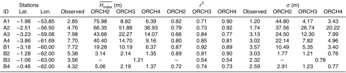
period. The effect of the change from the old distribution of the MFF (ORCH2) to the new one (ORCH3) and the effect of the calibration at OBI (ORCH4) on the simulated water level height is also shown (Table 7). Water height of the floodplains is not directly considered because ORCHIDEE does not take into account the height of the river bed. Then, an index of water height variation is performed for simulation and observations
15
data. The minimal value of the water height during the 8 yr is considered as the height of the river bed and it is consequently subtracted each month to the water level height from the simulated and observed data.
Over the main stem, water height level is highly overestimated at the four stations (A1 to A4) with the old distribution of MFF (ORCH2) according to Table 7. Moreover,
20
the overestimated standard deviation indicates a too-high variation in simulated water height through the year, despite a good correlation with observations. The new distri-bution of MFF (ORCH3) increases the rate of MFF over the main stem and logically reduces the water height of the floodplains. The calibration (ORCH4) improves the mean water height for the four stations (Table 7) and gives better correlations with
ob-25
HESSD
8, 11171–11232, 2011Amazon discharge simulation using ORCHIDEE forced by
new datasets
M. Guimberteau et al.
Title Page
Abstract Introduction
Conclusions References
Tables Figures
◭ ◮
◭ ◮
Back Close
Full Screen / Esc
Printer-friendly Version
Interactive Discussion
Discussion
P
a
per
|
Dis
cussion
P
a
per
|
Discussion
P
a
per
|
Discussio
n
P
a
per
with Topex/Poseidon measurements with a small overestimation. This corroborates the findings by Hess et al. (2003) who estimate only 5 % more of MFF than ORCHIDEE at Cabaliana near MANA (see Fig. 6).
Over the Rio Negro, the change of the distribution in MFF does not improve the correlation with measurements which is good near the main stem at B1 and B2 (about
5
0.9) and low at B3 and B4 (between 0.5 and 0.7) (Table 7). We note that no fraction of floodplains were present in the old map at station B3, whereas the new distribution now enables a comparison with observations. The water height is underestimated at all the stations when compared to measurements, for all the simulations except B1 close to the main stem. In fact, the interannual seasonality of water height of floodplains is
10
well captured at this station with ORCH4 compared to measurements during the eight years (Fig. 17). The old distribution in MFF largely overestimates the water height in flooded areas.
6 Summary and final remarks
In this work, the simulation by ORCHIDEE of discharge values in the main tributaries of
15
the Amazon River basin and in the last gauged station ´Obidos has benefited from two major inputs. A first improvement results from the introduction of a comprehensive daily rainfall observations derived from HYBAM dataset, that includes data from upstream regions of the basin, especially in Bolivia, Peru, Ecuador and Colombia that were not taken into consideration in former simulations. Indeed, the addition of high rainfall in
20
the northwestern equatorial region and in some rainy spots spread along the Andes tends to improve the mean rainfall over the basin (ORCH2) that was previously un-derestimated (ORCH1). Simulated evapotranspiration remains unun-derestimated when using HYBAM rainfall forcing, but the use of daily values in precipitation seems to highly improve the seasonal variation of evaporation of water over the leaves (ORCH2) when
25