www.hydrol-earth-syst-sci.net/19/3771/2015/ doi:10.5194/hess-19-3771-2015
© Author(s) 2015. CC Attribution 3.0 License.
Transit times from rainfall to baseflow in headwater catchments
estimated using tritium: the Ovens River, Australia
I. Cartwright1,2and U. Morgenstern3
1School of Earth, Atmosphere and Environment, Monash University, Clayton, Vic. 3800, Australia
2National Centre for Groundwater Research and Training, GPO Box 2100, Flinders University, Adelaide, SA 5001, Australia 3GNS Science, Lower Hutt 5040, New Zealand
Correspondence to: I. Cartwright ([email protected])
Received: 29 April 2015 – Published in Hydrol. Earth Syst. Sci. Discuss.: 11 June 2015 Revised: 28 August 2015 – Accepted: 31 August 2015 – Published: 8 September 2015
Abstract. Headwater streams contribute a significant propor-tion of the total flow to many river systems, especially dur-ing summer low-flow periods. However, despite their impor-tance, the time taken for water to travel through headwater catchments and into the streams (the transit time) is poorly understood. Here,3H activities of stream water are used to define transit times of water contributing to streams from the upper reaches of the Ovens River in south-east Australia at varying flow conditions. 3H activities of the stream water varied from 1.63 to 2.45 TU, which are below the average
3H activity of modern local rainfall (2.85 to 2.99 TU). The
highest 3H activities were recorded following higher win-ter flows and the lowest3H activities were recorded at sum-mer low-flow conditions. Variations of major ion concentra-tions and3H activities with streamflow imply that different stores of water from within the catchment (e.g. from the soil or regolith) are mobilised during rainfall events rather than there being simple dilution of an older groundwater com-ponent by event water. Mean transit times calculated using an exponential-piston flow model range from 4 to 30 years and are higher at summer low-flow conditions. Mean transit times calculated using other flow models (e.g. exponential flow or dispersion) are similar. There are broad correlations between3H activities and the percentage of rainfall exported from each catchment and between3H activities and Na and
Cl concentrations that allow first-order estimates of mean transit times in adjacent catchments or at different times in these catchments to be made. Water from the upper Ovens River has similar mean transit times to the headwater streams implying there is no significant input of old water from the alluvial gravels. The observation that the water contributing
to the headwater streams in the Ovens catchment has a mean transit time of years to decades implies that these streams are buffered against rainfall variations on timescales of a few years. However, impacts of any changes to land use in these catchments may take years to decades to manifest themselves in changes to streamflow or water quality.
1 Introduction
Documenting the timescales over which rainfall is transmit-ted through catchments to streams (the transit time) is critical for understanding catchment hydrology and for the protec-tion and management of river systems. While there has been an increasing number of studies that have estimated transit times (e.g. Kirchner et al., 2010; McDonnell et al., 2010; Morgenstern et al., 2010, 2015; Hrachowitz et al., 2013), the time taken for water to be transformed from rainfall to stream baseflow remains poorly understood in many catch-ments. Likewise the factors that control variations in transit times between catchments are not well documented.
sys-tems. The observation that many headwater streams continue to flow over prolonged dry periods indicates, however, that these catchments contain stores of water in soils, weathered rocks, or fractures with retention times of at least a few years (e.g. Maloszewski and Zuber, 1982; Maloszewski et al., 1992; Rice and Hornberger, 1998; Maloszewski, 2000). However, the transit times of water within these stores and whether different stores are more active at different times, for example during high vs. low rainfall periods, is not well known.
At times of low flow, much of the water in streams and rivers is likely derived from long-term stores such as ground-water (Sophocleous, 2002; McCallum et al., 2010; Cook, 2013). Less well understood is the extent to which older wa-ter rather than event wawa-ter (i.e. that derived from recent rain-fall) contributes to higher streamflows. In some catchments at least, rainfall appears to displace water from the soils and regolith and increase groundwater inflows to streams due to hydraulic loading. In these cases relatively old water may still contribute a significant volume of water to the river at higher streamflows (Sklash and Farvolden, 1979; Rice and Horn-berger, 1998; Kirchner, 2009; Hrachowitz et al., 2011).
Understanding the timescales of water movement within headwater catchments is an essential part of water manage-ment. Headwater streams contribute a significant proportion of the total flow of many river systems (Freeman et al., 2007). Thus the water provided by headwater streams is that which may be eventually used downstream for domestic use, recre-ation, agriculture, and/or industry. Many headwater catch-ments retain native vegetation; however, increasing popula-tion growth and economic development has seen progressive changes of land use, including plantation forestry, agricul-ture, and urban development. The impacts of such develop-ment on the headwater catchdevelop-ments, and consequently on the river systems as a whole, is currently poorly understood.
Identifying first-order controls on transit times aids the prediction of likely transit times in adjacent catchments. Ge-ology, vegetation, and soil types, which influence recharge rates and groundwater fluxes, may be important controls on transit times. Catchment area and the drainage density (the length of stream per unit area of catchment) may also be im-portant controls on transit times (Morgenstern et al., 2015). Larger catchments are likely to have longer flow paths which result in longer transit times. However, if the catchment con-tains a higher density of streams there may be numerous short flow paths between recharge areas and discharge points in the streams. Additionally, transit times may correlate with the proportion of rainfall exported from the catchment by the stream (the runoff coefficient). This is because catchments with low runoff coefficients are likely to have higher evap-otranspiration rates which lead to low infiltration rates and relatively slow passage of water through the catchment.
1.1 Determining water transit times
There are several methods that may be used to estimate the time taken for water to transit through a catchment to the stream. The temporal variation of stable isotope ratios and/or major ion concentrations in rainfall become attenuated with increasing transit times as mixing of water derived from dif-ferent rainfall episodes occurs within the catchment (Kirch-ner, 2009; Kirchner et al., 2010; Hrachowitz et al., 2013). When combined with lumped parameter models that describe the distribution of residence times along flow paths in a catchment (e.g. Maloszewski and Zuber, 1982; Maloszewski, 2000), the variation in geochemistry at the catchment out-let can be used to quantify water transit times. While this methodology has been applied with some success, there are some limitations. Firstly, it requires detailed (preferably at least weekly) stable isotope and/or major ion geochemistry data for rainfall collected over a period which exceeds that of the transit times of water in the catchment. Such data are not commonly available, especially where transit times are more than a few years. Secondly, a single estimate of the transit time is commonly estimated for the catchment whereas water with different transit times may contribute to the stream at low and higher flows (e.g. Morgenstern et al., 2010, 2015). Seasonal variations in flow within the catch-ment may also attenuate variations in the concentrations of these tracers (Kirchner, 2015). Finally, these tracers are pro-gressively more ineffective where transit times are in ex-cess of 4-5 years as the temporal variations are smoothed out (Stewart et al., 2010).
Tritium (3H), which has a half-life of 12.32 years, may also be used to determine transit times of relatively young (<100 years) groundwater into streams using lumped pa-rameter models. 3H is part of the water molecule and its abundance in water is only affected by initial activities and radioactive decay, and not by reactions between the water and the aquifer matrix, as is the case with some solute trac-ers such as14C or32Si. Other potential tracers such as3He, the chlorofluorocarbons, and SF6 are gases that equilibrate
with the atmosphere and are difficult to use in streams. The
3H activities in rainfall have been measured globally for
the Southern Hemisphere have decayed well below those of modern rainfall. This situation results in unique transit times being estimated from single3H measurements (Morgenstern et al., 2010; Morgenstern and Daughney, 2012), which in turn permits the transit time of water contributing to streams at specific flow conditions to be determined.
There is always uncertainty in calculating transit or res-idence times using lumped parameter models as they are a simplification of the flow system. However, since the bomb-pulse 3H has mostly disappeared in the Southern Hemi-sphere,3H activities reflect relative transit times that do not depend on the applicability of the assumed model (i.e. wa-ter with low3H activities has longer mean transit times than water with high 3H activities). This allows 3H activities to be readily compared with other parameters (e.g. streamflow or major ion compositions). By contrast, as discussed above, for Northern Hemisphere waters individual3H activities do not yield unique residence times and comparisons can only be made with transit times derived from time series of 3H activities that are inherently model dependant.
1.2 Qualitative water transit time indicators
In many catchments, including the Ovens, the concentration of major ions in groundwater increases with time (Edmunds et al., 1982; Bullen et al., 1996; Zuber et al., 2005; Mor-genstern et al., 2010; Cartwright and MorMor-genstern, 2012). Thus, major ion concentrations in stream water can also pro-vide an indication of the relative transit time of water that contributes to the stream. There may also be a correlation between streamflow and transit times (Morgenstern et al., 2010). As major ion concentrations and streamflow data are easier to obtain than3H activities and commonly already ex-ist, such correlations offer the possibility of providing first-order estimates of transit times in adjacent catchments or to periods when no3H activities were measured.
1.3 Aims and objectives
The aim of this paper is to understand the transit times of baseflow, here defined as including all non-surface wa-ter sources including soil wawa-ter, inwa-terflow, and groundwawa-ter, contributing to headwater streams in the Ovens catchment, south-east Australia using 3H activities and major ion con-centrations. Specifically, we use these data to test the follow-ing hypotheses. Firstly, that transit times in individual catch-ments vary with streamflow as different water stores in the catchments are mobilised. Secondly, that there are first-order controls on transit times, such as catchment area, geology, land use, catchment size, or the runoff coefficient. Finally, that the concentration of major ions will increase with resi-dence time in the catchment and can be used as proxies for the transit time. While this study is based in the Ovens catch-ment, understanding the first order controls on water transit times or whether there are proxies that may be used to
es-Wa
Br
UBK LBK MY
BR
UMC SM
Sampling Site Locality My
25 km
SA QLD
VIC
NSW
a
Granite
Shepparton Ordovician-Devonian
Alluvial Sediments
LMC
OWB SC
OEB Mt B
RP
MY
RP
Catchment Boundary
River
Basement
}
OvensVictorian Alps 37oS
36o 20’S
147oE 146o 20’E
36o 40’S
146o 60’E
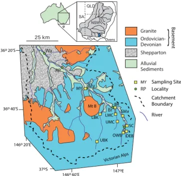
Figure 1. Summary geological and location map of the Ovens catchment, data from Energy and Earth Resources (2015). Sam-pling sites: BR=Bright, LBK=Lower Buckland, LMC=Lower Morses Creek, MY=Myrtleford, OEB=Ovens East Branch, OWB=Ovens West Branch, SC=Simmons Creek, SM=Smoko, UBK=Upper Buckland, UMC=Upper Morses Creek. Localities: Br=Bright, Ha=Harrietville, My=Myrtleford, Mt B=Mount Buffalo; RP=Rocky Point, Wa=Wangaratta. Inset map shows location of Ovens Valley relative to the Murray-Darling Basin
(shaded); NSW=New South Wales, QLD=Queensland,
SA=South Australia, VIC=Victoria.
timate transit times has an application to other catchments globally.
2 Setting
The Ovens River is part of the Murray-Darling River sys-tem (Lawrence, 1988). The Ovens River is perennial with a length of approximately 200 km and its headwaters extend into the Victorian Alps (Fig. 1). It has a single channel con-fined within a steep-sided valley south (upstream) of Myrtle-ford and then develops into a network of meandering and anastomosing channels north of Wangaratta prior to its con-fluence with the Murray River. This study concentrates on the upper reaches of the Ovens catchment upstream of Myrtle-ford (Fig. 1), which includes several headwater tributaries, notably the Buckland River, Morses Creek, and the East and West Branches of the Ovens River.
weathered zones mainly close to the land surface (Shugg, 1987; van den Berg and Morand, 1997). The basement rocks are overlain by sediments of the Quaternary Shepparton For-mation and the Holocene Coonambidgal ForFor-mation that in this area are contiguous and indistinguishable. These two for-mations occur in the river valleys and comprise unconsoli-dated and generally poorly sorted immature fluvio-lacustrine sands, gravels, silts and clays (Tickell, 1978; Shugg, 1987; Lawrence, 1988). The Shepparton and Coonambidgal For-mations increase in thickness away from the Victorian Alps and reach a maximum thickness of 170 m in the lower Ovens Valley; however, where present in the upper Ovens catch-ment, they are<50 m thick and thin out considerably in the tributary valleys. The hydraulic conductivity of the Shep-parton and Coonambidgal Formations varies from 0.1 to 60 m day−1 with typical values of 0.2 to 5 m day−1
(Tick-ell, 1978; Shugg, 1987). Alluvial fans that are locally tens of metres thick and which comprise of coarse-grained poorly sorted immature sediments commonly occur between the basement rocks and the floodplain.
The upper reaches of the Ovens River and its tributaries are characterised by narrow steep-sided valleys that are dom-inated by native eucalyptus forest with subordinate pine plan-tations. The Ovens Valley broadens downstream of Harri-etville (Fig. 1) and alluvial flats up to 2 km wide are devel-oped adjacent to the Ovens River and in the lower reaches of the tributaries. These alluvial flats together with some of the alluvial fans have been cleared for agriculture, which includes cattle grazing, orchards, vineyards, hops, and fruit farms. The population of the upper Ovens Valley is∼7500, mainly in the towns of Myrtleford, Bright, and Harrietville. This part of the Ovens catchment contains no reservoirs and, while there is some use of surface and groundwater, the flow regimes in the upper Ovens catchment are considered to be little impacted (Goulburn-Murray Water, 2015).
Average precipitation decreases from 1420 mm yr−1in the alpine region to 1170 mm yr−1at Bright (Bureau of Meteo-rology, 2015). Approximately 45 % of the annual precipita-tion occurs in the austral winter (June to September) with a proportion of the winter precipitation occurring as snow on the higher peaks, while March has the lowest precipita-tion (5 to 6 % of the annual total). Streamflow in the Ovens River at Bright (Fig. 1) between 1924 and 2014 was between 1000 and 3.28×10⁷m3day−1with high flows occurring in winter (Department of Environment and Primary Industries, 2015).
3 Sampling and analytical methods 3.1 Sampling sites
The sampling sites in this study have been designated as being from headwater catchments or floodplain areas. The headwater catchment areas are dominantly composed of
basement rocks covered with eucalyptus forest and subor-dinate plantation forest. Alluvial sediments in these catch-ments are restricted to zones of a few metres to tens of me-tres wide immediately adjacent to the streams. The Ovens East Branch (catchment area of 72 km2), Ovens West Branch (catchment area of 42 km2), and Simmons Creek (catchment area of 6 km2) were sampled at Harrietville close to where these streams enter the floodplain of the Ovens Valley. The upper Buckland River (catchment area of 77 km2) and upper Morses Creek (catchment area of 32 km2) are from the up-per reaches of those tributaries that are largely undeveloped. The lower Buckland River (catchment area of 435 km2) and lower Morses Creek (catchment area of 123 km2) have some land clearing on the lower parts of alluvial fans and the flood-plain. Together these streams represent the main tributaries in the upper Ovens Valley (Fig. 1).
The floodplain sites are on the main Ovens River (Fig. 1, Table 1). Here the floodplain is up to 2 km wide and is un-derlain by coarse-grained alluvial sediments that are up to 50 m thick. The floodplain and some of the lower slopes of the alluvial fans have been cleared while the upper slopes are still dominated by eucalyptus forests with subordinate pine plantations. The Smoko (catchment area of 267 km2) and Bright (catchment area of 302 km2) sampling sites are upstream of the junction with Morses Creek and downstream of the Ovens East Branch, Ovens West Branch and Simmons Creek tributaries. The Myrtleford sampling site (catchment area of 1240 km2) is downstream of the junction with the Buckland River and upstream of the junction with the Buf-falo River (not sampled in this study). Sampling took place in four rounds (Table 1, Fig. 2) that represent a variety of flow conditions.
3.2 Streamflow measurements
Streamflow is monitored at or close to the Myrtleford, Bright, Ovens West Branch (until 1989), Simmons Creek, Lower Buckland, and Lower Morses Creek sampling sites (Depart-ment of Environ(Depart-ment and Primary Industries, 2015). A gauge at Harrietville (Fig. 1) records the combined streamflow from the Ovens West Branch and Ovens East Branch tributaries. The average daily combined streamflow at Harrietville and that of the Ovens West Branch are well correlated over a wide range of flows (n=1012, R2=0.97) allowing the stream-flow of the Ovens West Branch for the sampling rounds in this study to be calculated from the Harrietville streamflow. In turn, this enables the contribution of Ovens East Branch tributary to the combined flows to be estimated.
3.3 Geochemical sampling
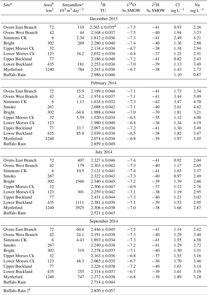
Table 1. Geochemistry of the Ovens River and tributaries.
Sitea Areab Streamflowc 3H δ18O δ2H Cl Na
km2 103m3day−1 TU ‰ SMOW ‰ SMOW mg L−1 mg L−1
December 2013
Ovens East Branch 72 110 2.265±0.035d −7.5 −41 0.93 2.26
Ovens West Branch 42 44 2.168±0.037 −7.5 −40 1.94 3.23
Simmons CK 6 2.34 1.812±0.036 −7.3 −41 2.49 4.21
Bright 302 269 2.280±0.040 −7.4 −40 1.36 2.88
Upper Morses Ck 32 2.134±0.036 −6.7 −38 1.18 2.94
Lower Morses Ck 123 34.2 2.032±0.036 −6.8 −37 1.25 2.91
Upper Buckland 77 2.186±0.040 −7.2 −41 0.82 3.43
Lower Buckland 435 181 2.253±0.036 −7.0 −39 1.13 3.49
Myrtleford 1240 784 2.243±0.036 −6.7 −38 1.43 2.72
Buffalo Rain 2.986±0.046 1.10 0.87
February 2014
Ovens East Branch 72 15.9 2.189±0.046 −7.1 −41 1.73 3.34
Ovens West Branch 42 4.2 1.974±0.037 −7.1 −41 3.44 5.49
Simmons CK 6 1.13 1.634±0.032 −7.3 −42 3.47 4.78
Smoko 267 2.088±0.042 −7.1 −40 2.61 4.62
Bright 302 64.6 1.988±0.044 −7.0 −39 1.81 3.21
Upper Morses Ck 32 5.59 1.920±0.034 −6.5 −35 1.12 4.08
Lower Morses Ck 123 1.980±0.040 −6.4 −36 1.34 4.19
Upper Buckland 77 33.7 2.097±0.036 −7.2 −41 1.36 3.49
Lower Buckland 435 85.8 2.039±0.036 −6.5 −38 1.82 3.47
Myrtleford 1240 2.074±0.036 −6.8 −39 1.97 3.45
Buffalo Rain 2.859±0.049
July 2014
Ovens East Branch 72 407 2.327±0.046 −7.4 −41 0.92 2.04
Ovens West Branch 42 179 2.303±0.042 −7.3 −40 1.17 2.65
Simmons CK 6 10.5 2.121±0.041 −7.4 −41 1.63 3.37
Smoko 267 2.322±0.043 −7.3 −40 0.97 2.49
Bright 302 1566 2.340±0.045 −7.2 −39 1.39 2.66
Upper Morses Ck 32 2.306±0.047 −6.9 −37 1.12 2.76
Lower Morses Ck 123 301 2.259±0.042 −7.1 −38 1.19 2.95
Upper Buckland 77 2.431±0.044 −7.3 −40 1.21 3.02
Lower Buckland 435 1111 2.381±0.039 −7.1 −39 1.53 2.95
Myrtleford 1240 3925 2.306±0.038 −7.0 −38 1.66 2.87
Buffalo Rain 2.521±0.043
September 2014
Ovens East Branch 72 60.6 2.446±0.045 −7.5 −41 1.14 2.42
Ovens West Branch 42 24.1 2.191±0.038 −7.3 −40 1.29 3.40
Simmons CK 6 4.43 1.893±0.034 −7.3 −41 1.55 4.58
Smoko 267 2.240±0.038 −7.2 −41 1.29 2.72
Bright 302 319 2.278±0.037 −7.1 −40 1.50 3.31
Upper Morses Ck 32 2.163±0.036 −6.8 −37 1.55 3.16
Lower Morses Ck 123 48.3 2.065±0.035 −6.7 −36 1.70 3.46
Upper Buckland 77 2.226±0.038 −7.2 −40 1.63 3.14
Lower Buckland 435 255 2.314±0.037 −6.7 −39 1.61 3.19
Myrtleford 1240 747 2.272±0.038 −6.8 −39 1.89 3.28
Buffalo Rain 2.714±0.044
Buffalo Rain 2f 2.850±0.057
aLocalities on Fig. 1.bArea of catchment upstream of sampling site.cRiver discharge. Discharge for Ovens East Branch and Ovens West Branch
estimated from the Harrietville gauge as discussed in text.dThe tritium error is individually calibrated and calculated for each sample as described by
5x10⁴
100
0 10 20 30 40 50 60 70 80 90 100 Dec 13 Feb 14 Jul 14 Oct 14
Str
eamflo
w (m
3 da
y
-1)
Year % Time Exceeded
a b
Bright 5x10⁶
5x10⁵
101 102 103 104
2010 2011 2012 2013 2014
Sampling campaigns
Figure 2. (a) Flow of the Ovens River at Bright between 2009 and 2014, arrows show timing of sampling campaigns. (b) Flow duration curve for Bright. Data from Department of Environment Primary Industries (2015).
using a ThermoFinnigan ICP-OES or ICP-MS on samples that had been filtered through 0.45 µm cellulose nitrate filters and acidified to pH<2 using double-distilled 16 M HNO3.
Anions were analysed on filtered unacidified samples using a Metrohm ion chromatograph at Monash University. The pre-cision of anion and cation analyses based on replicate anal-yses is±2 % and the accuracy based on analysis of certified water standards is±5 %. While a range of major ion concen-trations were measured only Cl and Na, which represent the major anion and cation in surface water and groundwater, are discussed here. Additional major ion data are from the Department of Environment and Primary Industries (2015).
Stable isotopes were measured at Monash University using Finnigan MAT 252 and ThermoFinnigan DeltaPlus Advan-tage mass spectrometers. δ18O values were determined via equilibration with He-CO2 at 32◦C for 24–48 h in a
Ther-moFinnigan Gas Bench.δ2H was measured by reaction with Cr at 850◦C using an automated Finnigan MAT H/Device. δ18O andδ2H values were measured relative to internal stan-dards calibrated using IAEA SMOW, GISP and SLAP. Data were normalized following (Coplen, 1988) and are expressed relative to V-SMOW. Precision (1σ) based on replicate anal-ysis is δ18O= ±0.1 ‰ and δ2H= ±1 ‰. 3H activities are expressed in tritium units (TU) where 1 TU represents a
3H /1H ratio of 1
×10−18. Samples for3H were vacuum dis-tilled and electrolytically enriched prior to being analysed by liquid scintillation spectrometry using Quantulus ultra-low-level counters at GNS, New Zealand. Following from Mor-genstern and Taylor (2009) the sensitivity is now further in-creased to a lower detection limit of 0.02 TU via tritium richment by a factor of 95, and reproducibility of tritium en-richment of 1 % is achieved via deuterium-calibration for ev-ery sample. The precision (1σ) is∼1.8 % at 2 TU (Table 1). 3.4 Estimating mean transit times using3H
Water flowing through an aquifer follows flow paths of varying length, which results in the water discharging into streams having a range of transit times rather than a dis-crete age. The mean transit times may be calculated us-ing the lumped parameter models described by Maloszewski
and Zuber (1982, 1992), Cook and Bohlke (2000), Mal-oszewski (2000) and Zuber et al. (2005) that treat the dis-charging water as comprising numerous aliquots each of which has followed a different flow path and thus taken a dif-ferent amount of time to pass through the aquifer. For steady-state groundwater flow, the activity of3H in water discharg-ing into the stream at timet(Co(t )) is related to the input of 3H (C
i) over time via the convolution integral:
Co(t )= ∞ Z
0
Ci(t−τ )g(τ )e−λτdτ, (1)
whereτ is the transit time,t−τ is the time that the water entered the flow system,λis the decay constant (0.0563 yr−1 for3H), andg(τ )is the response function that describes the distribution of flow paths and transit times in the system.
The exponential flow model describes the mean transit time in homogeneous unconfined aquifers of constant thick-ness that receive uniform recharge and where flow paths from the entire aquifer thickness discharge to the stream. Piston flow assumes linear flow with no mixing within the aquifer, such that all water discharging to the stream at any one time has the same transit time. The exponential-piston flow model describes mean transit times in aquifers that have regions where flow paths have an exponential distribution and re-gions where flow paths have a linear distribution. For the exponential-piston flow modelg(τ )in Eq. (1) is given by: g(τ )=0 forτ < τm(1−f ) (2a)
g(τ )=(f τm)−1e−τ/f τm+1/f−1forτ > τm(1−f ), (2b)
whereτm is the mean transit time and f is the proportion
an alternative lumped parameter model based on the one-dimensional advection-dispersion transport in a semi-infinite medium. The response function for this model is:
g(τ )= 1 τ√4π DPτ/τm
e−
(1−τ/τm)2
4DPτ/τm
, (3)
where DP is the dispersion parameter (unitless), which is
the inverse of the more commonly reported Peclet Number. DP=D/(v x), wherev is velocity (m day−1),x is distance
(m), and D is the dispersion coefficient (m2day−1). While the dispersion model is considered to be a less realistic con-ceptualisation of flow systems, it commonly reproduces the observed distribution of radioisotopes within aquifers (Mal-oszewski, 2000).
3.5 Mass balance calculations
If groundwater and rainfall have different major ion con-centrations, stable isotope ratios, or3H activities, variations in these parameters with streamflow may be used to assess the degree of mixing of baseflow with event water (Sklash and Farvolden, 1979; Uhlenbrook et al., 2002; Godsey et al., 2009). In the case where baseflow to the stream remains rel-atively constant and increases in streamflow are due to addi-tional event water, the proportion of baseflow in the stream (Xbf) is given byQbf/QwhereQis the measured
stream-flow andQbf is the streamflow at baseflow conditions. The
concentration of a component in the stream (Cst) at higher
streamflows is given by:
Cst=XbfCbf+(1−Xbf) Cew, (4)
whereCbfandCeware the concentrations in the baseflow and
event water, respectively.
4 Results
4.1 Streamflow variations
Figure 2a summarises the variation in streamflow at Bright between 2010 and 2014 and Fig. 2b shows the distribution of the sampling rounds relative to the flow frequency curve for 1980 to 2014 daily streamflow at Bright. The July 2014 sampling round was during a recession period from winter high flows and the streamflow of 1.57×10⁶m3day−1
rep-resents the 5.5 percentile of streamflow (i.e. streamflow of this value or higher was recorded on 5.5 % of days during 1980 to 2014). The December 2013 and October 2014 sam-pling rounds represent periods of intermediate streamflow of 2.69×10⁵and 3.19×10⁵m3day−1, which correspond to the 46.3 and 42.1 percentiles of streamflow, respectively. The February 2014 sampling round represents typical late austral summer low-flow conditions. The streamflow at Bright dur-ing this sampldur-ing round of 6.46×10⁴m3day−1was close to
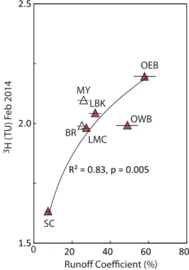
R² = 0.83, p = 0.005
1.5 2.0 2.5
20 40 60 80
Runoff Coefficient (%) 3H (
TU) F
eb 2014
SC
OEB
OWB BR
MY
LMC LBK
0
Figure 3. Runoff coefficient vs.3H activities for February 2014. Bars show range of runoff coefficients arising from the likely range of rainfall in the catchments, line is a logarithmic fit to the data that has an R2 of 0.83. Open symbols are sampling sites on the main Ovens River, closed symbols are from the headwater tributaries. BR=Bright, LBK=Lower Buckland, LMC=Lower Morses Creek, OEB=Ovens East Branch, OWB=Ovens West Branch, SC=Simmons Creek. Data from Tables 1 and 2; precision of3H activities (Table 1) is approximately the size of the symbols.
the minimum streamflow for the 2013 to 2014 summer of 5.44×10⁴m3day−1 (Department of Environment and Pri-mary Industries, 2015) and represents the 86.4 percentile of streamflow between 1980 and 2014.
f: Lower Buckland River d: Bright
1.4 1.6 1.8 2 2.2 2.4 2.6 2.8 3
e: Lower Morses Creek
1.4 1.6 1.8 2 2.2 2.4 2.6 2.8 3
c: Simmons Creek
b: Ovens West Branch
1.4 1.6 1.8 2 2.2 2.4 2.6 2.8 3
a: Ovens East Branch
1.4 1.6 1.8 2 2.2 2.4 2.6 2.8 3
g: Myrtleford
Dec 13 Feb 14 Jul 14 Oct 14
Streamflow (m3 day-1) 3H (
TU) 103 104 105
103 104 105 106
103 104 105 106
104 105 106 107
104 105 106 107
104 105 106 107
104 105 106
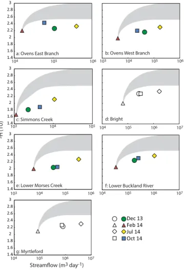
Figure 4. 3H activities vs. streamflow for the main Ovens River (open symbols) and its headwater tributaries (closed symbols); data from Table 1. Shaded fields depict mixing between baseflow, which is assumed to have a3H activity of the lowest streamflow at each site, and rainfall with a 3H activity of between 2.5 and 3.0 TU, which spans the range of rainfall3H activities in Table 1 constructed using Eq. (4). The mixing model overestimates the 3H activities recorded at higher flows at all sites.
4.2 3H activities
The rainfall sample from December 2013 represents a
∼17 month aggregate sample from Mount Buffalo and has a 3H activity of 2.99 TU (Table 1). A second 12 month aggregate sample collected from a different site on Mount Buffalo in March 2015 has a 3H activity of 2.85 TU (Ta-ble 1). These 3H activities are close to those expected for modern rainfall in south-east Australia (Tadros et al., 2014). Shorter timescale (2 to 5 month) rainfall samples collected from Mount Buffalo in February 2014, July 2014, and Octo-ber 2014 have3H activities between 2.52 and 2.89 TU. The lowest3H activities from the rainfall are from rainfall col-lected between February and July 2014 in the austral autumn. Autumn and winter rains are commonly depleted in3H (Mor-genstern et al., 2010; Tadros et al., 2014) as the main3H
in-1.5 2 2.5 3
1 10 100 1000 10,000
Dec 13 Feb 14 Jul 14 Oct 14
Catchment area (km2) 3H (
TU)
MY LBK BR SM
SC
UMC OWB UBK OEB
LMC
17 month average
Rainfall
12 month average
Figure 5. 3H activities vs catchment area for the main Ovens River (open symbols) and its headwater tributaries (closed sym-bols) and the range of rainfall3H activities (aggregated rainfall samples shown by solid arrows, other rainfall samples by dashed arrows); data from Table 1. BR=Bright, LBK=Lower Buckland, LMC=Lower Morses Creek, MY=Myrtleford, OEB=Ovens East Branch, OWB=Ovens West Branch, SC=Simmons Creek, SM=Smoko, UBK=Upper Buckland, UMC=Upper Morses Creek. Precision of3H activities (Table 1) is approximately the size of the symbols.
jection into the troposphere occurs in early spring. Stream water samples have3H activities between 1.63 and 2.43 TU (Table 1), which are lower than all of the rainfall samples.
The highest3H activities of stream water at each sampling site are generally from the high-flow conditions in July 2014, while the lowest 3H activities are from the February 2014 low-flow period (Table 1, Figs. 4 and 5). The 3H activi-ties from the three floodplain sites are similar to those of the headwater streams and there are no systematic down-stream trends along the main Ovens River. Likewise there is little systematic variation in3H activities downstream in the Buckland River and Morses Creek. There is also not a positive correlation between catchment area and3H
activ-ities (Fig. 5); indeed, Simmons Creek, which is the small-est catchment, records the lowsmall-est3H activities in each sam-pling round. There is, however, a broad correlation between the runoff coefficient and3H activities as illustrated for the February 2014 samples in Fig. 3, with a similar relationship apparent in the other sampling campaigns (Tables 1 and 2). 4.3 Major ion and stable isotope geochemistry
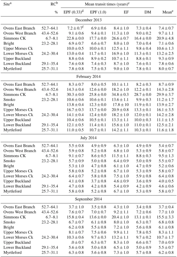
Table 2. Calculated mean transit times for the Ovens River baseflow.
Sitea RCb Mean transit times (years)c
% EPF (0.33)d EPF (1.0) EF DM Meane
December 2013
Ovens East Branch 52.7–64.1 7.2±0.7f 6.9±0.6 8.4±1.0 7.3±0.4 7.4±0.7
Ovens West Branch 43.4–52.6 9.1±0.6 9.4±0.1 11.3±1.0 9.0±0.2 9.7±1.1
Simmons CK 6.7–8.1 22.8±0.0 17.7±0.0 26.6±0.7 16.4±0.0 20.9±4.8
Bright 23.2–28.1 6.9±0.7 6.6±0.7 8.0±1.0 7.0±0.4 7.1±0.6
Upper Morses Ck 10.0±0.5 10.0±0.1 12.5±1.1 9.8±0.4 10.6±1.3
Lower Morses Ck 24.2–30.4 13.0±0.4 11.7±0.1 16.9±1.0 11.3±0.1 13.2±2.5
Upper Buckland 8.8±0.6 8.9±0.2 10.7±1.1 8.8±0.1 9.3±0.9
Lower Buckland 29.1–35.4 7.6±0.8 7.4±0.3 8.7±1.0 7.6±0.1 7.8±0.6
Myrtleford 25.7–31.1 7.8±0.8 7.5±0.3 9.0±1.0 7.8±0.1 8.0±0.7
February 2014
Ovens East Branch 52.7–64.1 8.3±0.7 8.0±0.5 10.1±1.1 8.2±0.3 8.7±0.9
Ovens West Branch 43.4–52.6 14.3±0.4 12.6±0.0 18.2±1.0 12.2±0.1 14.3±2.8
Simmons CK 6.7–8.1 30.3±0.0 25.8±0.0 34.8±0.3 28.7±0.0 29.9±3.7
Smoko 23.2–28.1 10.6±0.6 10.6±0.1 13.6±1.1 9.9±0.3 11.2±1.7
Bright 13.8±0.4 12.3±0.0 17.8±10 11.9±0.1 13.9±2.7
Upper Morses Ck 16.7±0.3 13.7±0.0 20.9±0.8 13.3±0.1 16.1±3.5
Lower Morses Ck 24.2–30.4 14.1±0.4 12.4±0.0 18.2±1.0 12.0±0.1 14.2±2.8
Upper Buckland 10.4±0.6 10.5±0.1 13.3±1.1 10.0±0.3 11.1±1.5
Lower Buckland 29.1–35.4 12.1±0.5 11.4±0.1 15.6±1.0 11.0±0.1 12.5±2.1
Myrtleford 25.7–31.1 11.0±0.5 10.7±0.1 14.2±1.1 10.3±0.1 11.6±1.8
July 2014
Ovens East Branch 52.7–64.1 5.5±0.8 4.9±0.9 6.3±1.0 4.9±0.9 5.4±0.7
Ovens West Branch 43.4–52.6 5.9±0.8 5.2±0.8 6.8±1.0 5.3±0.9 5.8±0.7
Simmons CK 6.7–8.1 9.1±0.7 8.6±0.5 11.5±1.1 8.8±0.3 9.5±1.3
Smoko 23.2–28.1 5.7±0.9 5.0±0.8 6.4±0.9 5.0±0.9 5.5±0.7
Bright 5.3±1.0 4.7±0.8 6.1±1.0 4.7±0.9 5.2±0.6
Upper Morses Ck 5.8±0.8 5.2±0.8 6.7±1.0 5.3±0.9 5.8±0.7
Lower Morses Ck 24.2–30.4 6.4±0.7 5.8±0.8 7.5±1.0 5.9±0.8 6.4±0.8
Upper Buckland 4.1±0.8 3.7±0.8 4.6±0.9 3.6±0.9 4.0±0.5
Lower Buckland 29.1–35.4 4.7±0.8 4.2±0.8 5.4±0.9 4.2±0.9 4.6±0.6
Myrtleford 25.7–31.1 5.8±0.8 5.2±0.8 6.7±1.0 5.3±0.9 5.8±0.7
September 2014
Ovens East Branch 52.7–64.1 3.7±1.0 3.5±0.8 4.3±1.0 3.4±0.8 3.7±0.4
Ovens West Branch 43.4–52.6 7.6±0.7 7.0±0.7 9.2±1.1 7.2±0.6 7.7±1.0
Simmons CK 6.7–8.1 15.8±0.4 13.6±0.0 20.4±1.0 13.1±0.1 15.5±3.3
Smoko 23.2–28.1 6.7±0.7 6.1±0.8 8.0±1.0 6.3±0.7 6.8±0.8
Bright 6.2±0.8 5.5±0.8 7.2±1.0 5.6±0.8 6.1±0.8
Upper Morses Ck 8.1±0.7 7.5±0.6 9.9±1.1 7.8±0.5 8.3±1.1
Lower Morses Ck 24.2–30.4 10.3±0.6 9.7±0.3 13.2±1.1 9.7±0.2 10.7±1.7
Upper Buckland .0±0.7 6.3±0.7 8.3±1.0 6.6±0.7 7.0±0.9
Lower Buckland 29.1–35.4 5.6±0.8 5.0±0.8 6.5±1.0 5.0±0.9 5.5±0.7
Myrtleford 25.7–31.1 6.3±0.8 5.6±0.8 7.3±1.0 5.7±0.8 6.2±0.8
aSites on Fig. 1.bRunoff coefficient, range reflects likely rainfall range in catchments.cLumped parameter models: EF=exponential
-46 -42 -38 -34
-8.0 -7.0 -6.0 -5.0
Dec 13 Feb 14 Jul 14 Oct 14 GMWL
δ18O (‰ V-SMOW)
δ
2H (‰
V
-SMOW
)
slope = 5.5
Figure 6.δ18O vs.δ2H values for the main Ovens River (open sym-bols) and its headwater tributaries (closed symsym-bols) in the four sam-pling rounds; GMWL=Global Meteoric Water Line. Data from Ta-ble 1.
to local climatic factors (Ivkovic et al., 1998; Leaney and Herczeg, 1999; Cartwright et al., 2012).
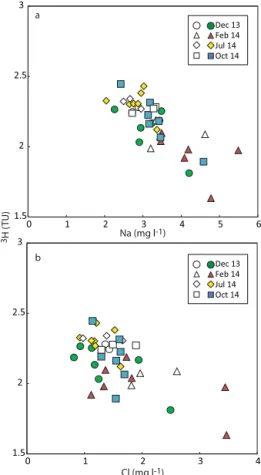
Na and Cl concentrations from the rainfall sample at Mount Buffalo are 0.97 and 1.1 mg L−1, respectively (Ta-ble 1), which are similar to the Na concentrations of 0.9 to 1.3 mg L−1and Cl concentrations 1.2 to 1.4 L−1reported for rainfall in this region of south-east Australia by Blackburn and McLeod (1983). Na and Cl concentrations in stream wa-ter from the Ovens catchment range from 2.4 to 5.5 mg L−1 and 0.82 to 3.5 mg L−1, respectively (Table 1). The con-centrations of these and other major ions are higher dur-ing low-flow periods (February 2014) than durdur-ing periods of higher flow. Na / Cl mass ratios of the stream samples are between 1.4 and 4.2 which are higher than the Na / Cl ra-tios of local rainfall of 0.7 to 0.9 (Table 1; Blackburn and McLeod, 1983). Since 3H activities are inversely correlated with streamflow (Figs. 4 and 5), there is also a broad inverse correlation between 3H activities and Cl and Na concentra-tions (Fig. 7).
A correlation between major ion concentrations and streamflow is also apparent on a longer timescale. Figure 8a shows the variation of streamflow and Na concentrations at Harrietville made as part of routine geochemical measure-ments (Department of Environment and Primary Industries, 2015). The Na concentrations range from 1.3 to 2.2 mg L−1 at high flows to∼4.4 mg L−1at low flows. As noted earlier, the Harrietville gauge records the combined streamflow from the Ovens East Branch and Ovens West Branch; however, the Na vs. streamflow trends for these two tributaries are similar to that from the Harrietville gauge (Fig. 8a), albeit with far less data.
5 Discussion
The combination of streamflow data, major ion concentra-tions, stable isotope geochemistry, and3H activities allow an
1.5 2 2.5
3
0 1 2 3 4 5 6
1.5 2 2.5
3
0 1 2 3 4
Dec 13 Feb 14 Jul 14 Oct 14
3H (
TU)
Cl (mg l-1)
Na (mg l-1)
a
b
Dec 13 Feb 14 Jul 14 Oct 14
Figure 7.3H activities vs. Na (a) and Cl (b) concentrations for the main Ovens River (open symbols) and its headwater tributaries (closed symbols) in the four sampling rounds. Data from Table 1.
understanding of the hydrogeology of the upper Ovens catch-ment to be made.
5.1 Changes to water stores with streamflow
One fundamental question relating to catchment hydrology is the extent to which water in streams at high flows is event wa-ter largely derived from recent rainfall rather than older wawa-ter displaced from stores within the catchment (Sklash and Far-volden, 1979; Rice and Hornberger, 1998; Uhlenbrook et al., 2002; Kirchner et al., 2010). Resolution of this question is important to interpreting3H activities. If significant dilution with event water occurs, any increases in3H activities in the stream with increasing flow (e.g. Figs. 4 and 5) may be the result of mixing between high3H event water and an older baseflow component, and the3H activities may be used to estimate the proportions of these two components (Morgen-stern et al., 2010). By contrast, if water is displaced from the catchment during high rainfall events, the3H activities will reflect the mean transit time of that water and differences in
3H activities with streamflow may reflect the mobilisation of
0 1 2 3 4 5 6
103 104 105 106
0 1 2 3 4 5 6 7
104 105 106 107 108
a: Harrietville
b: Rocky Point
Na (mg l
-1)
Streamflow (m3 day-1)
OWB OEB
Figure 8. Na concentrations vs. streamflow for Harrietville (a) and Rocky Point (b), data from the Department of Environment and Pri-mary Industries (2015). (a) also shows Na vs streamflow for the Ovens East Branch (OEB) and Ovens West Branch (OWB) tribu-taries which join just upstream of the Harrietville gauge (Fig. 1). Shaded fields depict mixing between baseflow, which is assumed to have a Na concentration of the lowest streamflow at each site, and rainfall with a Na concentration of 0.9 to 1.3 mg L−1calculated us-ing Eq. (4). The mixus-ing model underestimates the Na concentration recorded at higher flows at both locations.
In the upper Ovens Valley only the Harrietville gauge, which records the combined East Branch and West Branch streamflow, has sufficient major ion data to assess the de-gree of mixing of baseflow with event water. Figure 8a shows the calculated Na vs. streamflow trends resulting from the mixing of event water and baseflow at the Harrietville gauge using Eq. (4) and the following assumptions: (1) Na concentrations at the lowest streamflow represents the Na concentrations of baseflow; (2) the baseflow remains con-stant at the value of the minimum streamflow, in this case 6600 m3day−1; and (3) rainfall has an Na concentration
be-tween 0.9 and 1.3 mg L−1 (Blackburn and McLeod, 1983).
The calculated Na vs. mixing trend underestimates the ob-served Na concentrations in the stream at Harrietville. A similar conclusion is also made for Na concentrations at the Rocky Point gauge, which is∼25 km downstream of Myrtle-ford (Fig. 8b).
Similar conclusions may be made from the 3H activities, albeit the data sets are much smaller. Figure 4 shows
pre-dicted3H activities vs. streamflow trends constructed using
Eq. (4) with similar assumptions to those above, namely: (1) at low-flow conditions the streams derive all their water from baseflow that has 3H activities of the February 2014 sampling campaign; (2) baseflow remains constant at the streamflow recorded in February 2014; and (3) rainfall has a3H activity between 2.5 and 3.0 TU which spans the range of activities in Table 1. For all catchments the mixing trends overestimate the3H activities of the stream water.
That the Na / Cl ratios of all stream samples, even those at high streamflow, exceed those of rainfall implies that some Na is derived from the dissolution of minerals, probably predominantly plagioclase feldspar, from the soils, regolith, or bedrock. As mineral dissolution occurs over timescales months to years (Edmunds et al., 1982; Bullen et al., 1996; Morgenstern et al., 2010; Cartwright and Morgenstern, 2012) this observation is also consistent with the interpretation that much of the water in the stream has been mobilised from within the catchment.
δ18O andδ2H values of stream water define arrays with slopes of 4–6 (Table 1, Fig. 6) that most likely reflects a combination of instream evaporation, especially in Febru-ary 2014, and possibly the altitude effect where stream wa-ter derived from rainfall at higher altitudes has lowerδ18O andδ2H values (cf. Clark and Fritz, 1997). The observation that theδ18O andδ2H values are similar at different flows is consistent with the water contributing to the stream having been resident within the catchment for sufficient time that any seasonal variations in rainfallδ18O andδ2H values have homogenised by mixing.
Taken together the3H activities, major ion concentrations, and stable isotope values are most consistent with a signifi-cant component of water in the stream at all flow conditions being derived from stores within the catchment that have a transit time of several years. High rainfall results in increased recharge that displaces older water from the soils, regolith, and sediments into the stream. The variation in3H activities with streamflow (Fig. 4) probably reflects the variation in the transit times (discussed below) of water within these different stores and the variations in Na and Cl concentrations (Fig. 7) reflect differences in chemistry between the water stores in the catchment.
5.2 Transit times of stream water in the Ovens catchment
pis-0 5 10 15 20 25 30 35
0 1 2 3 4 5 6
MY LBK BR
SM SC UMC OWB UBK OEB
LMC
Na (mg l-1)
M
ean T
ransit T
ime
(yr)
Figure 9. Mean transit times calculated using the Exponential-Piston Flow model vs. Na concentrations for the sites in the Ovens catchment (data from Tables 1 and 2). There is a broad correlation between mean transit time and Na con-centration. BR=Bright, LBK=Lower Buckland, LMC=Lower Morses Creek, MY=Myrtleford, OEB=Ovens East Branch, OWB=Ovens West Branch, SC=Simmons Creek, SM=Smoko, UBK=Upper Buckland, UMC=Upper Morses Creek.
ton flow (Cook and Bohlke, 2000; Morgenstern et al., 2010). Initial calculations were carried out for f=0.75 (EPM ra-tio=0.33). Based on the variations of geochemistry with streamflow (Figs. 3 and 8) it was assumed that the water con-tributing to the streams during all sampling campaigns was from baseflow. If the stream contains some event water that is diluting the baseflow, this approach will yield a minimum transit time for the baseflow component.
The3H input function is based on the annual average3H activities of rainfall in Melbourne collected for the Interna-tional Atomic Energy Agency Global Network of Isotopes in Precipitation program as summarised by Tadros et al. (2014). The3H activities of the two aggregated rainfall samples from the Ovens Valley of 2.85 and 2.99 TU (Table 1) are used to bracket the present-day rainfall3H activities. Rainfall3H activities reached∼62 TU in 1965 and then declined expo-nentially to present-day values by ∼1995.3H activities of 2.85 and 2.99 TU were also used for the pre-atmospheric nu-clear test precipitation.
The exponential-piston flow model yields unique mean transit times for the range of measured3H activities in the Ovens catchment (Table 2, Fig. 9). The longest mean tran-sit times at each tran-site are from the low-flow period in Febru-ary 2014 and range from 8 years at Ovens East Branch to 30 years at Simmons Creek. Stream water from the two Morses Creek sites has mean transit times of 14 to 17 years while mean transit times of stream water from the two Buck-land River sites are 10 to 12 years. Mean transit times from the high-flow period (July 2014) calculating using the same
exponential-flow model are between 4 years at Upper Buck-land and 9 years at Simmons Creek (Table 2, Fig. 9). Mean transit times in the intermediate flow periods are between 7 and 23 years for December 2013 and 4 and 16 years for September 2014. In both these sampling campaigns Sim-mons Creek recorded the longest mean transit times while the shortest mean transit times were at Bright (December 2013) and Ovens East Branch (September 2014).
There are several uncertainties in these calculations that need to be assessed. Firstly, the calculated transit times vary with the choice of model (Table 2). Using the exponential-piston flow model withf=0.5 (EPM ratio=1), which rep-resents an aquifer system with equal portions of piston and exponential flow, yields mean transit times that range from 8 to 26 years in February 2014 and 4 to 9 years in July 2014. Using the exponential flow model (f=1, EPM ratio=0), yields mean transit times that range from 10 to 35 years in February 2014 and 5 to 12 years in July 2014. The dispersion model withDP=0.1 yields mean transit times between 8 and
29 years in February 2014 and 4 to 9 years in July 2014. The absolute difference between the results from the models in-creases with the mean transit time. For the highest3H activity of 2.45 TU (Ovens East Branch in September 2014) the aver-age mean transit time from the four models is 3.7±0.4 years. For the lowest 3H activity of 1.63 TU (Simmons Creek in February 2014) the average mean transit time from the four models is 29.9±3.8 years.
Allowing the 3H activity of modern rainfall to vary be-tween 2.85 and 2.99 also results in uncertainties in the calculated mean transit times. For the exponential-piston flow model with f=0.75, the standard deviation of the mean transit times decreases from ∼1.0 years at 4 years to <0.1 years at >20 years, while the standard deviation of the mean transit times for the exponential-piston flow model with f=0.5 decreases from ∼0.9 years at 4 years to<0.1 years at >10 years. The standard deviation of the mean transit times in the exponential flow model decreases from∼0.9 years at 4 years to∼0.3 years at 35 years but has a maximum value of∼1.1 years at 10 to 15 years, whereas the standard deviation of the mean transit times in the dispersion model decreases from∼0.9 years at 4 years to<0.1 years at 12 years. These differences reflect differences in the exit-age frequency distribution in the various models (e.g. Cook and Bohlke, 2000).
The analytical uncertainty of the3H activities produces uncertainties in the calculated mean transit times. The
rainfall3H activities before and during the bomb pulse have
less impact than any uncertainties in the modern3H activities of rainfall.
Finally, the lumped parameter models are only an approx-imation of the flow through aquifer systems and real flow systems will differ to a greater or lesser extent. However, this will have little impact on the calculated variation in mean transit times in individual catchments at different stream-flows as the flow systems within a specific catchment will likely be similar over time. Hence, while there are uncertain-ties in the calculated mean transit times, the conclusions that the mean transit times at the lowest flow conditions are on the order of years to decades while at higher flow conditions the mean transit times are at least a few years remain unaffected.
5.3 Controls on transit times
The mean transit times do not increase with catchment area and the smallest catchment (Simmons Creek) records the longest transit times (up to 30 years in February 2014). There is little difference in the geology or topography of the head-water sites implying that these are not factors which ex-plain the variation in transit times between the catchments. Drainage density can influence transit times as it controls the distance between groundwater recharge areas and the nearest point of discharge in the stream (Morgenstern et al., 2015). In the case of the upper Ovens catchment, there is little differ-ence in drainage density between the catchments, and many of the larger catchments have areas that are larger than the Simmons Creek catchment (∼6 km2) which are devoid of streams that flow during summer. These observations imply that drainage density is not the main control on transit times. River water from the three floodplain sites along the main Ovens Valley (Smoko, Bright, and Myrtleford) have mean transit times that are not appreciably different from that of many of the headwater streams (Figs. 3 and 4), implying that there is not a large store of deep older groundwater con-tributing to baseflow in this stretch of the Ovens River. This conclusion is consistent with observations that the3H activ-ities of shallow (<40 m) groundwater from the alluvial sed-iments in the Ovens Valley between Myrtleford and Bright are>1 TU with most having3H activities between 1.5 and 2.5 TU (Cartwright and Morgenstern, 2012).
There is a broad correlation between transit times and the runoff coefficient (Fig. 3). Evapotranspiration during recharge is a dominant hydrological process in south-east Australia and the native eucalyptus vegetation in particular has very high transpiration rates (Allison et al., 1990; Her-czeg et al., 2001; Cartwright et al., 2012). While the catch-ments are similar, subtle differences in soil type which con-trols the rate of infiltration, vegetation density, or regolith thickness may influence evapotranspiration rates (Cartwright et al., 2006). Infiltration rates will vary inversely with the de-gree of evapotranspiration and catchments with high
evapo-transpiration rates are likely to contribute smaller volumes of relatively old water to the streams draining those catchments. Regardless of the cause, the correlation between the runoff coefficient and3H activities allows a first-order estimation of likely transit times in similar catchments to be made which is useful for management purposes. The correlation between Na and Cl concentrations and3H activities (Figs. 7 and 9) suggests that major ion geochemistry can also provide a first-order indication of the mean transit times of baseflow. That the trends in Na ion concentrations and mean transit times from the different catchments overlap (Fig. 9) indicates that this approach may be useful in adjacent catchments with sim-ilar geology, topography, and vegetation.
6 Conclusions and implications
This study has demonstrated the utility of high-precision3H measurements in determining mean transit times of water in headwater catchments. The observation that the water con-tributing to the headwater streams in the Ovens catchment has mean transit times of years to decades implies that these streams are buffered against rainfall variations on timescales of a few years, and most of these streams continued to flow through the 1996–2010 Millennium drought (Bureau of Me-teorology, 2015; Department of Environment and Primary Industries, 2015). However, the impacts of any changes to land use in these catchments or longer-term rainfall changes may take years to decades to manifest itself in changes to streamflow or water quality. If the conclusion that the mean transit times are controlled by the evapotranspiration rates in the catchments is correct, large-scale vegetation changes, for example replacing native forest by grassland that has lower transpiration rates, will cause a significant change in tran-sit times. Specifically, lower transpiration rates will increase recharge that will likely result in development of shallow flow paths with short transit times and also increase the flow velocities in the deeper flow paths due to increased hydraulic heads. Both of these factors will likely reduce the mean tran-sit times.
Author contributions. Both authors were involved in the design and
realisation of the sampling program. U. Morgenstern carried out the 3H analyses and I. Cartwright oversaw the analysis of the other
geo-chemical parameters. I. Cartwright prepared the manuscript with contributions from U. Morgenstern.
Acknowledgements. Funding for this project was provided by
helped with the geochemical analyses at Monash University. Two anonymous reviewers and the editor (M. Hrachowitz) provided encouraging and helpful comments.
Edited by: M. Hrachowitz
References
Allison, G. B., Cook, P. G., Barnett, S. R., Walker, G. R., Jolly, I. D., and Hughes, M. W.: Land clearance and river salinisation in the western Murray Basin, Australia, J. Hydrol., 119, 1–20, 1990. Blackburn, G. and McLeod, S.: Salinity of atmospheric
precipita-tion in the Murray Darling Drainage Division, Australia, Austr. J. Soil Res., 21, 400–434, 1983
Bullen, T. D., Krabbenhoft, D. P., and Kendall, C.: Kinetic and min-eralogic controls on the evolution of groundwater chemistry and 87Sr/86Sr in a sandy silicate aquifer, northern Wisconsin, USA,
Geochim. Cosmochim. Acta, 60, 1807–1821, 1996.
Bureau of Meteorology: Commonwealth of Australia Bureau of Meteorology, available at: http://www.bom.gov.au, last access: March 2015.
Cartwright, I. and Morgenstern, U.: Constraining groundwater recharge and the rate of geochemical processes using tritium and major ion geochemistry: Ovens catchment, southeast Australia, J. Hydrol., 475, 137–149, 2012.
Cartwright, I., Weaver, T. R., Cendón, D. I., Fifield, L. K., Tweed, S. O., Petrides, B., and Swane, I.: Constraining groundwater flow, residence times, inter-aquifer mixing, and aquifer properties us-ing environmental isotopes in the southeast Murray Basin, Aus-tralia, Appl. Geochem., 27, 1698–1709, 2012.
Cartwright, I., Weaver, T. R., and Fifield, L. K.: Cl / Br ratios and environmental isotopes as indicators of recharge variability and groundwater flow: An example from the southeast Murray Basin, Australia, Chem. Geol., 231, 38–56, 2006.
Clark, I. D. and Fritz, P.: Environmental Isotopes in Hydrogeology, Lewis, New York, USA, 328 pp., 1997.
Cook, P. G.: Estimating groundwater discharge to rivers from river chemistry surveys, Hydrol. Process., 27, 3694–3707, 2013. Cook, P. G. and Bohlke, J. K.: Determining timescales for
ground-water flow and solute transport, in: Environmental Tracers in Subsurface Hydrology, edited by: Cook, P. G. and Herczeg, A. L., Kluwer, Boston, USA, 1–30, 2000.
Coplen, T. B.: Normalization of oxygen and hydrogen isotope data, Chem. Geol., 72, 293–297, 1988.
Department of Environment and Primary Industries: Victoria De-partment of Environment and Primary Industries Water Moni-toring, available at: http://data.water.vic.gov.au/monitoring.htm, last access: March 2015.
Edmunds, W. M., Bath, A. H., and Miles, D. L.: Hydrochemical evolution of the East Midlands Triassic sandstone aquifer, Eng-land, Geochim. Cosmochim. Acta, 46, 2069–2081, 1982.
Energy and Earth Resources: State Government
Victo-ria Energy and Earth Resources, available at: http: //www.energyandresources.vic.gov.au/earth-resources/
maps-reports-and-data/geovic, last access: March 2015. Freeman, C. M., Pringle, C. M., and Jackson, C. R.: Hydrologic
connectivity and the contribution of stream headwaters to
eco-logical integrity at regional scales, J. Am. Water Resour. As., 43, 5–14, 2007.
Goulburn-Murray Water: Ovens Basin, available at: http://www. g-mwater.com.au/water-resources/catchments/ovensbasin, last access: April 2015.
Godsey, S. E., Kirchner, J. W., and Clow, D. W.: Concentration– discharge relationships reflect chemostatic characteristics of US catchments, Hydrol. Process., 23, 1844–1864, 2009.
Herczeg, A. L., Dogramaci, S. S., and Leaney, F. W.: Origin of dis-solved salts in a large, semi-arid groundwater system: Murray Basin, Australia, Mar. Freshwater Res., 52, 41–52, 2001. Hrachowitz, M., Bohte, R., Mul, M. L., Bogaard, T. A., Savenije,
H. H. G., and Uhlenbrook, S.: On the value of combined event runoff and tracer analysis to improve understanding of catchment functioning in a data-scarce semi-arid area. Hydrol. Earth Syst. Sci., 15, 2007–2024, doi:10.5194/hess-15-2007-2011, 2011. Hrachowitz, M., Savenije, H., Bogaard, T. A., Tetzlaff, D., and
Soulsby, C.: What can flux tracking teach us about water age dis-tribution patterns and their temporal dynamics?, Hydrol. Earth Syst. Sci., 17, 533–564, doi:10.5194/hess-17-533-2013, 2013. International Atomic Energy Association: Global Network of
Iso-topes in Precipitation, available at: http://www.iaea.org/water, last access: February 2015.
Ivkovic, K. M., Watkins, K. L., Cresswell, R. G., and Bauld, J.: A Groundwater Quality Assessment of the Upper Shepparton For-mation Aquifers: Cobram Region, Victoria, Austr. Geol. Surv. Org. Record 1998/16, Austr. Geol. Surv. Org., Canberra, Aus-tralia, 1998.
Jurgens, B.C., Bohlke, J. K., and Eberts, S. M.: Trac-erLPM (Version 1): An Excel® workbook for interpreting groundwater age distributions from environmental tracer data, US Geol. Surv. Techniques and Methods Report 4-F3, US Ge-ological Survey, Reston, USA, 60 pp., 2012.
Kirchner, J. W.: Catchments as simple dynamical systems: Catchment characterization, rainfall-runoff modeling, and do-ing hydrology backward, Water Resour. Res., 45, W02429, doi:10.1029/2008WR006912, 2009.
Kirchner, J. W.: Aggregation in environmental systems: catchment mean transit times and young water fractions under hydrologic nonstationarity, Hydrol. Earth Syst. Sci. Discuss., 12, 3105– 3167, doi:10.5194/hessd-12-3105-2015, 2015.
Kirchner, J. W., Tetzlaff, D., and Soulsby, C.: Comparing chloride and water isotopes as hydrological tracers in two Scottish catch-ments, Hydrol. Process., 24, 1631–1645, 2010.
Lawrence, C. R.: Murray Basin, in: Geology of Victoria, edited by: Douglas J. G. and Ferguson, J. A., Geological Society of Aus-tralia (Victoria Division), Melbourne, AusAus-tralia, 352–363, 1988. Leaney, F. and Herczeg, A.: The origin of fresh groundwater in the SW Murray Basin and its potential for salinisation, CSIRO Land and Water Technical Report 7/99, CSIRO, Adelaide, Australia, 1999.
Maloszewski, P.: Lumped-parameter models as a tool for deter-mining the hydrological parameters of some groundwater sys-tems based on isotope data, IAHS-AISH Publication 262, Vi-enna, Austria, 271–276, 2000.
Maloszewski, P. and Zuber, A.: On the calibration and validation of mathematical models for the interpretation of tracer experiments in groundwater, Adv. Water Resour., 15, 47–62, 1992.
Maloszewski, P., Rauert, W., Trimborn, P., Herrmann, A., and Rau, R.: Isotope hydrological study of mean transit times in an alpine basin (Wimbachtal, Germany), J. Hydrol., 140, 343–360, 1992. McCallum, J. L., Cook, P. G., Brunner, P., and Berhane, D.:
So-lute dynamics during bank storage flows and implications for chemical base flow separation, Water Resour. Res., 46, W07541, doi:10.1029/2009WR008539, 2010.
McDonnell, J. J., McGuire, K., Aggarwal, P., Beven, K. J., Biondi, D., Destouni, G., Dunn, S., James, A., Kirchner, J., Kraft, P., Lyon, S., Maloszewski, P., Newman, B., Pfister, L., Rinaldo, A., Rodhe, A., Sayama, T., Seibert, J., Solomon, K., Soulsby, C., Stewart, M., Tetzlaff, D., Tobin, C., Troch, P., Weiler, M., Western, A., Wörman, A., and Wrede, S.: How old is streamwa-ter? Open questions in catchment transit time conceptualization, modelling and analysis, Hydrol. Process., 24, 1745–1754, 2010. Morgenstern, U. and Daughney, C. J.: Groundwater age for iden-tification of baseline groundwater quality and impacts of land-use intensification – The National Groundwater Monitoring Pro-gramme of New Zealand, J. Hydrol., 456–457, 79–93, 2012. Morgenstern, U. and Taylor, C. B.: Ultra low-level tritium
mea-surement using electrolytic enrichment and LSC, Isot. Environ. Healt. S., 45, 96–117, 2009.
Morgenstern, U., Stewart, M. K., and Stenger, R.: Dating of streamwater using tritium in a post nuclear bomb pulse world: Continuous variation of mean transit time with streamflow, Hy-drol. Earth Syst. Sci., 14, 2289–2301, doi:10.5194/hess-14-2289-2010, 2010.
Morgenstern, U., Daughney, C. J., Leonard, G., Gordon, D., Donath, F. M., and Reeves, R.: Using groundwater age and hydrochemistry to understand sources and dynamics of nu-trient contamination through the catchment into Lake Ro-torua, New Zealand, Hydrol. Earth Syst. Sci., 19, 803–822, doi:10.5194/hess-19-803-2015, 2015.
Rice, K. C. and Hornberger, G. M.: Comparison of hydrochemical tracers to estimate source contributions to peak flow in a small, forested, headwater catchment, Water Resour. Res., 34, 1755– 1766, 1998.
Shugg, A.: Hydrogeology of the Upper Ovens Valley, Victoria De-partment of Industry, Technology and Resources Report 1987/5, Melbourne, Australia, 1987.
Sklash, M. G. and Farvolden, R. N.: The role of groundwater in storm runoff, J. Hydrol., 43, 45–65, 1979.
Sophocleous, M.: Interactions between groundwater and surface water: the state of the science, Hydrogeol. J., 10, 52–67, 2002. Stewart, M. K., Morgenstern, U., and McDonnell, J. J.:
Trunca-tion of stream residence time: How the use of stable isotopes has skewed our concept of streamwater age and origin, Hydrol. Process., 24, 1646–1659, 2010.
Tadros, C. V., Hughes, C. E., Crawford, J., Hollins, S. E., and Chis-ari, R.: Tritium in Australian precipitation: A 50 year record, J. Hydrol., 513, 262–273, 2014.
Tickell, S. J.: Geology and hydrogeology of the eastern part of the riverine plain in Victoria, Geological Survey of Victoria Re-port 1977-8, Melbourne, Australia, 73 pp., 1978,
Uhlenbrook, S., Frey, M., Leibundgut, C., and Maloszewski, P.: Hydrograph separations in a mesoscale mountainous basin at event and seasonal timescales, Water Resour. Res., 38, 311– 3114, 2002.
van den Berg, A. H. M. and Morand, V.: Wangaratta, Geological Survey of Victoria 1 : 250,000 Geological Map Series, Geologi-cal Survey of Victoria, Melbourne, Australia, 1997.
Winter, T. C.: Relation of streams, lakes, and wetlands to ground-water flow systems, Hydrogeol. J., 7, 28–45, 1999.