www.geosci-model-dev.net/9/2223/2016/ doi:10.5194/gmd-9-2223-2016
© Author(s) 2016. CC Attribution 3.0 License.
mizuRoute version 1: a river network routing tool for a continental
domain water resources applications
Naoki Mizukami1, Martyn P. Clark1, Kevin Sampson1, Bart Nijssen2, Yixin Mao2, Hilary McMillan3,8,
Roland J. Viger4, Steve L. Markstrom4, Lauren E. Hay4, Ross Woods5, Jeffrey R. Arnold6, and Levi D. Brekke7 1National Center for Atmospheric Research, Boulder, CO, USA
2University of Washington, Seattle, WA, USA
3National Institute of Water and Atmospheric Research, Christchurch, New Zealand 4United States Geological Survey, Denver, CO, USA
5University of Bristol, Bristol, UK
6U.S. Army of Corps of Engineers, Seattle, WA, USA 7Bureau of Reclamation, Denver, CO, USA
8San Diego State University, San Diego, CA, USA
Correspondence to:Naoki Mizukami ([email protected])
Received: 8 September 2015 – Published in Geosci. Model Dev. Discuss.: 2 November 2015 Revised: 25 March 2016 – Accepted: 1 June 2016 – Published: 23 June 2016
Abstract. This paper describes the first version of a stand-alone runoff routing tool, mizuRoute. The mizuRoute tool post-processes runoff outputs from any distributed hydro-logic model or land surface model to produce spatially dis-tributed streamflow at various spatial scales from headwater basins to continental-wide river systems. The tool can utilize both traditional grid-based river network and vector-based river network data. Both types of river network include river segment lines and the associated drainage basin polygons, but the vector-based river network can represent finer-scale river lines than the grid-based network. Streamflow estimates at any desired location in the river network can be easily ex-tracted from the output of mizuRoute. The routing process is simulated as two separate steps. First, hillslope routing is performed with a gamma-distribution-based unit-hydrograph to transport runoff from a hillslope to a catchment outlet. The second step is river channel routing, which is performed with one of two routing scheme options: (1) a kinematic wave tracking (KWT) routing procedure; and (2) an impulse re-sponse function – unit-hydrograph (IRF-UH) routing pro-cedure. The mizuRoute tool also includes scripts (python, NetCDF operators) to pre-process spatial river network data. This paper demonstrates mizuRoute’s capabilities to produce spatially distributed streamflow simulations based on river networks from the United States Geological Survey (USGS)
Geospatial Fabric (GF) data set in which over 54 000 river segments and their contributing areas are mapped across the contiguous United States (CONUS). A brief analysis of model parameter sensitivity is also provided. The mizuRoute tool can assist model-based water resources assessments in-cluding studies of the impacts of climate change on stream-flow.
1 Introduction
net-work across the domain of interest at each time step, facili-tating further spatial and temporal analysis of the estimated streamflow. As opposed to other routing models, our goal in developing mizuRoute is to provide flexibility in mak-ing routmak-ing model decisions (i.e., river network definition and routing scheme).
The paper proceeds as follows. Section 2 reviews ex-isting river routing models. Section 3 describes how the mizuRoute tool provides flexibility of routing modeling deci-sions and details the hillslope and river routing schemes used in mizuRoute. Section 4 provides an overview of the work-flow of mizuRoute from preprocessing hydrologic model output to simulating streamflow in the river network. Sec-tion 5 demonstrates streamflow simulaSec-tions in river systems over the contiguous United States (CONUS). Finally, a sum-mary and future work are discussed in Sect. 6.
2 Existing river routing models
The water resources and Earth system modeling commu-nities have developed a wide spectrum of river routing schemes of varying complexity (Clark et al., 2015). For ex-ample, the US Army Corps of Engineers (USACE) has de-veloped a stand-alone river modeling system called Hydro-logic Engineering Center – River Analysis System (HEC-RAS; Brunner, 2001). HEC-RAS offers various hydraulic routing schemes, ranging from simple uniform flow to one-dimensional (1-D) Saint-Venant equations for unsteady flow. HEC-RAS has been popular among civil engineers for river channel design and floodplain analysis where surveyed river geometry and physical channel properties are available. At the continental to global scale, unit-hydrograph approaches have been used (e.g., Nijssen et al., 1997; Lohmann et al., 1998; Goteti et al., 2008; Zaitchik et al., 2010; Xia et al., 2012), though more recent, large-scale river models use fully dynamic flow equations (e.g., Miguez-Macho and Fan, 2012; Paiva et al., 2013; Clark et al., 2015), simplified Saint-Venant equations such as the kinematic wave or diffusive wave equa-tion (e.g., Arora and Boer, 1999; Lucas-Picher et al., 2003; Koren et al., 2004; Yamazaki et al., 2011; Li et al., 2013; Yamazaki et al., 2013; Gochis, 2015; Yucel et al., 2015) or non-dynamical hydrologic routing methods such as Musk-ingum routing (e.g., David et al., 2011). Despite their com-putational cost, dynamic or diffusive wave models are attrac-tive for relaattrac-tively flat floodplain regions such as along the Amazon River where backwater effects on the flood wave are significant (Paiva et al., 2011; Yamazaki et al., 2011; Miguez-Macho and Fan, 2012). At the other end of the spec-trum, simpler, non-dynamic routing schemes, such as the unit-hydrograph approach, estimate the flood wave delay and attenuation, but do not simulate other streamflow variables such as flow velocity and flow depth.
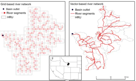
One of the key issues for large-scale river routing, besides the choice of the routing scheme, is the degree of
abstrac-tion in the representaabstrac-tion of the river network (Fig. 1). A vector-based representation of the river network refers to a collection of hydrologic response units (HRUs or spatially discretized areas defined in the model) that are delineated based on topography or catchment boundary. River segments in the vector-based river network, represented by lines, me-ander through HRUs and connect upstream with downstream HRUs. On the other hand, in the grid-based river network, the HRU is defined by a grid box and river segments con-nect neighboring grid boxes based on the flow directions. Vector-based river networks are better than coarser resolution (e.g.,>1 km) gridded river networks at preserving fine-scale features of the river system such as tortuosity and drainage area, therefore representing more accurate sub-catchment ar-eas and river segment lengths.
For large-scale applications, many studies have developed and evaluated methods to upscale fine-resolution flow direc-tion grids (∼1 km or less) to a coarser resolution (∼10 km or more) to match hydrologic model resolution and/or reduce the cost of routing computations (e.g., O’Donnell et al., 1999; Fekete et al., 2001; Olivera et al., 2002; Reed, 2003; Davies and Bell, 2009; Wu et al., 2011, 2012). Earlier work (e.g., O’Donnell et al., 1999; Fekete et al., 2001; Olivera et al., 2002) focused on preserving the accuracy of the flow direc-tion at the coarser resoludirec-tion and therefore on an accurate representation of the drainage area. Newer upscaling meth-ods are designed to also preserve fine-scale flow path length (e.g., Yamazaki et al., 2009; Wu et al., 2011). More recent river routing models have also begun to employ vector-based river networks (Goteti et al., 2008; David et al., 2011; Paiva et al., 2011; Lehner and Grill, 2013; Paiva et al., 2013; Ya-mazaki et al., 2013).
3 Runoff routing in mizuRoute
repre-Figure 1.Comparison of 1/8◦(∼12 km) gridded river network and vector river network from United States Geological Survey (USGS) Geospatial Fabric for the upper part of Snake River basin (Viger, 2014).
sentation of the river system and routing scheme differences (equations and parameters) separately.
The mizuRoute tool uses a two-step process to route basin runoff. First, basin runoff is routed from each hillslope to the river channel using a gamma-distribution-based unit hydro-graph. This allows for the representation of ephemeral chan-nels or chanchan-nels too small to be included in the river network. Second, using one of the two channel routing schemes, the delayed flow from each HRU is routed to downstream river segments along the river network. The routing time step is the same as that of the runoff output from the hydrologic model, typically an hourly or daily time step. The following sub-sections provide descriptions of the two routing steps. 3.1 Hillslope routing
Hillslope routing accounts for the time of concentration (Tc) of a HRU to estimate temporally delayed runoff (or dis-charge) at the outlet of the HRU from runoff computed by a hydrologic model.
For hillslope routing, mizuRoute uses a simple two-parameter Gamma distribution as a unit-hydrograph to route instantaneous runoff from a hydrologic model to an outlet of HRU. The Gamma distribution is expressed as
γ (t:a, θ )= 1 Ŵ (a) θat
a−1e−tθ, (1)
wheret is time [T],ais a shape parameter [–] (a >0), and θis a timescale parameter [T]. Both the shape and timescale parameters affect the peak time (mode of the distribution: (a−1)θ )and flashiness (variance of the distribution:aθ2)of the unit-hydrograph and depend on the physical HRU char-acteristics. Convolution of the gamma distribution with the runoff depth series is used to compute the fraction of runoff at the current time, which is discharged to its corresponding
river segment at each future time as follows:
q (t )= tmax Z
0
γ (s:a, θ )×R (t−s)ds, (2)
whereq is delayed runoff or discharge [L3T−1] at time step t[T],Ris HRU total runoff depth [L3T−1] from the hydro-logic model, andtmax is the maximum time length for the gamma distribution [T].
This two-parameter gamma distribution has been widely used in unit-hydrograph-based models for water resources engineering applications (e.g., Bhunya et al., 2007; Nadara-jah, 2007). Kumar et al. (2007) presented methods to esti-mate the two parameters in the gamma distribution based on geomorphological information. The gamma distribution offers a parsimonious way to describe a wide range of hillslope-to-channel responses in a computationally efficient manner, which is important for continental-scale domains. 3.2 River channel routing
Two different river channel routing schemes are implemented in mizuRoute: (1) KWT routing and (2) IRF-UH rout-ing. Both schemes are based on the one-dimensional (1-D) Saint-Venant equations that describe flood wave propagation through a river channel. The 1-D conservation equations for continuity (Eq. 3) and momentum (Eq. 4) are
∂q ∂x+
∂A
∂t =0, (3)
∂v ∂t +v
∂v ∂x+g
∂y
∂x−g(S0−Sf)=0, (4)
v is velocity [LT−1],y is depth of flow [L],S
0 is channel slope [–],Sfis friction slope [–], andgis gravitational con-stant [LT−2]. The continuity equation (Eq. 3) assumes that no lateral flow is added to a channel segment. The following sub-sections describe the two routing schemes.
3.2.1 Kinematic wave tracking (KWT)
In contrast with several other kinematic routing models that solve a kinematic wave equation with numerical schemes (e.g., Arora and Boer, 1999; Lucas-Picher et al., 2003; Koren et al., 2004), the KWT method computes a wave speed or a celerity for the runoff (or discharge) that enters an individual stream segment from the corresponding HRU at each time step using kinematic approximation (Goring, 1994; Clark et al., 2008). The runoff, represented as a particle, is propagated through the river network based on a travel time (the celerity divided by the segment length). Note that the wave celerity differs from the flow velocity, as the wave typically moves faster than water mass (McDonnell and Beven, 2014).
In the kinematic wave approximation with the assumption that the channel is rectangular and hydraulically wide (chan-nel width≫y), the wave celerity C [LT−1] is a function of channel width w[L], Manning’s coefficientn [–], chan-nel slope S0 [–], and discharge q [L3T−1]. Further details are provided in Appendix A. Among the four variables, the channel slope S0is provided by the river network data and discharge is computed with hillslope routing for the head-water basin, or/and updated via routing from the upstream segment. The other two variables, Manning’s coefficient n and river width w, are much more difficult to measure or estimate. The river width is determined with the following width–drainage area relationship (Booker, 2010):
w=Wa·Abups, (5)
where Wa is a width factor [–],Aups is the total upstream basin area [L2], andbis an empirical exponent equal to 0.5. The width factor Wa and the Manning’s coefficient n are treated as model parameters as shown in Table 1.
The KWT routing starts with ordering all the segments in the processing sequence from upstream to downstream. The KWT routing is performed at each segment in the processing order at each time step. The procedures of the KWT routing method are as follows:
1. Obtain the information on the waves that reside in the segment at a given time step: This includes the waves routed from the upstream segments, the wave that re-mains in this current segment form the previous time step, and the wave generated from the runoff from lo-cal HRUs during the current time step. Three state vari-ables of the waves are kept in the memory: (i) discharge; (ii) the time at which the wave enters the segment; and (iii) the time at which the wave is expected to exit the segment. At the first time step, only the wave from lo-cal HRUs exists. Figure 2a visualizes the discharge of
Figure 2.Visualization of waves. The top panel(a)plots a discharge of the wave [m3s−1] against its location (distance [km] from the
beginning of the 1st segment) at the beginning of five consecutive daily time steps. A vertical line indicates the river segment bound-ary. The bottom panel(b)plots a discharge of the wave [m3s−1]
against its exit time (day from 1 October) for the 4th and 13th seg-ments. A vertical line indicates the boundary of routing time step. The inserted map shows the 16 river segments used for the plots.
waves that reside in the 16 segments (16 river segments are shown in the inserted map) at the beginning of five time steps against the wave locations in the segments. 2. Remove waves in order to reduce the memory usage and
the processing time for the wave routing (the next step). The number of the waves in the segment is limited to a predefined number (20 by default). In Fig. 2, the thresh-old for the number of waves in each segment is set to 100. To determine which waves can be removed, the difference between the discharge of the wave and the linearly interpolated discharge between its two neigh-boring waves is computed for all waves, and the wave that produces the least difference (from the interpolated discharge) is removed so that loss of wave mass is min-imized. This process is repeated until the number of waves is below the threshold.
Table 1.Routing model parameters.
Parameters Routing methods Descriptions Values used in Sect. 5
a Hillslope Shape factor [–] 2.5 [–] θ Hillslope Timescale factor [T] 86 400 [s] n KWT Manning coefficient [–] 0.01 [–] W KWT River width scale factor [–] 0.001 [–] C IRF-UH Wave velocity [LT−1] 1.5 [ms−1] D IRF-UH Diffusivity [L2T−1] 800 [m2s−1]
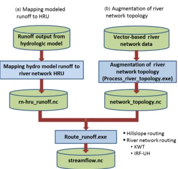
Figure 3.Overview of streamflow simulation with mizuRoute. The green cylinder and blue box denote data and computational process, respectively.
wave is expected to exit the river segment is updated. If the exit time occurs before the end of the time step, the wave is propagated to the downstream segment and flagged as “exited”. The exit time then becomes the time the wave entered the downstream segment. Otherwise, the wave is flagged as “not-exited”, and remains in the current segment. Figure 2b shows the discharge of the waves against the exit times of the corresponding waves at segments 4 and 13. As a reference, the end of each time step is shown as a vertical line.
The routing routine checks for (and corrects) the spe-cial case of a kinematic shock. A kinematic shock is a sudden rise in the flow depth, and thus an increase in the discharge at a fixed location, and occurs when a faster-moving wave successively overtakes multiple slower-waves to build a steep wave front. It occurs in models due to the kinematic approximation; in reality, diffusion would act to reduce the steepness of the wave front. Two neighboring waves are evaluated to check
if a slower wave is overtaken by a faster wave before the waves exit the river segment. If this occurs, those two waves are merged into one, and the celerity of the merged wave is updated with the following equation: Cmerge=
1q
1A=
1q
w1y, (6)
whereCmerge is the merged wave celerity [LT−1],1q and 1A are differences in discharge [L3T−1] and cross sectional flow area [L2T−1], respectively, be-tween slower and faster waves. Note that Eq. (6) is the mathematical definition of the wave celerity. Since we assume a rectangular channel, whose width is constant for each segment, the merged celerityCmergeis a func-tion of flow depthy, which is computed with Eq. (A4). 4. Finally, the time-step-averaged discharge (streamflow)
is computed by temporal integration of the discharge of all the waves that exit the segment during the time step. Temporal integral of wave discharge is visualized in Fig. 2b) as the area enclosed by the discharge curve formed by all the waves that exit during the time step. 3.2.2 Impulse response function – unit hydrograph
(IRF-UH)
The IRF-UH method mimics the river routing model of Lohmann et al. (1996), which has been used to route flows from gridded land surface models such as the Variable Infil-tration Capacity model (VIC; Liang et al., 1994). The only difference between the current tool and the Lohmann rout-ing tool is the way in which the river network is defined. The Lohmann routing model is designed as a grid-based model as shown in Fig. 1 to ease the coupling with grid-based land surface models. In mizuRoute, the same IRF-UH method can be used either on a vector- or grid-based river network. The descriptions of IRF-UH are given briefly as follows.
The mathematical developments of IRF-UH are based on 1-D diffusive wave equation derived from the 1-D Saint-Venant equations (Eqs. 3 and 4):
∂q ∂t =D
∂2q ∂x2−C
∂q
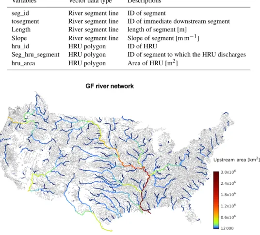
Table 2.River network information required in mizuRoute.
Variables Vector data type Descriptions
seg_id River segment line ID of segment
tosegment River segment line ID of immediate downstream segment Length River segment line length of segment [m]
Slope River segment line Slope of segment [m m−1]
hru_id HRU polygon ID of HRU
Seg_hru_segment HRU polygon ID of segment to which the HRU discharges hru_area HRU polygon Area of HRU [m2]
Figure 4. GF river network color coded by upstream drainage areas. Gray lines indicate the total upstream drainage areas less than 12 000 km2.
where parametersC andDare wave celerity [LT−1] and diffusivity [L2T−1], respectively. The complete derivation from Eqs. (3) and (4) to Eq. (7) is given in Appendix B.
Equation (7) can be solved using convolution integrals
q= t Z
0
U (t−s) h (x, s)ds, (8)
where
h (x, t )= x
2t√π Dtexp −
(Ct−x)2 4Dt
!
(9)
andU (t−s)is a unit depth of runoff generated at timet−s. This solution is a mathematical representation of the IRF used in unit-hydrograph theory. Wave celerityC and diffu-sivityDare treated as input parameters for this tool (Table 1), and ideally they can be estimated from observations of dis-charge and channel geometries at gauge locations.
Given a river segment or outlet segment, a set of unique unit-hydrographs is constructed for all the upstream seg-ments based on the distance between the upstream segment
and the outlet segment (Eq. 9). The unit-hydrograph convo-lution with delayed flow (i.e., hillslope-routed flow) is com-puted for each upstream segment and then all the routed flows from the upstream segments are summed to obtain the streamflow at the outlet segment. As opposed to the KWT routing, the IRF-UH routing does not require the segment se-quence for the routing computation. In other words, the rout-ing can be performed in any order of the segments within a river network and for a given segment the unit-hydrograph convolution can be also performed in any order of its up-stream segments.
4 mizuRoute workflow
Figure 5.Spatially distributed daily streamflow on 15 July 1986 in the GF river network simulated with mizuRoute. Gray lines indicate flow less than 100 m3s−1. The streamflow time series shown in Fig. 6 are extracted at three USGS gauges A–C.
is done by taking the area-weighted runoff of the intersecting hydrologic model HRUs. We developed the python scripts to identify the intersected hydrologic model HRUs for each river network HRU and their fractional areas to the river net-work HRU area to assist with this process.
The second data pre-processing step is augmentation of the river network data set. Typical topological information in this data set is the immediate downstream segment for each seg-ment. While a river network can be fully defined based on information about the immediate downstream segment, the river routing schemes in mizuRoute require identification of all the upstream river segments. For this purpose, we have de-veloped a program that identifies all the upstream segments for each segment in the river network data based solely on
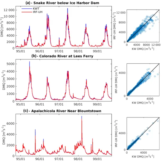
Figure 6.Daily mean streamflow (DMQ) at the three selected gauges in the GF river network. See Fig. 5 for the locations of the three gauges.
5 CONUS-wide mizuRoute simulations
The purpose of this section is to demonstrate the capa-bilities of mizuRoute to route multi-decadal runoff out-puts from hydrologic model simulations over the conti-nental domain. We use the United States Geological Sur-vey (USGS) Geospatial Fabric (GF) vector-based river net-work (Viger, 2014; http://wwwbrr.cr.usgs.gov/projects/SW_ MoWS/GeospatialFabric.html) over the CONUS. We routed the daily runoff simulations archived by Reclamation (2014) as part of their project “Downscaled CMIP3 and CMIP5 Cli-mate and Hydrology Projections” (http://gdo-dcp.ucllnl.org/ downscaled_cmip_projections/dcpInterface.html). In that project, the VIC model was forced by the spatially downscaled temperature and precipitation outputs at 1/8◦ (∼12 km) resolution from 97 global climate model outputs from 1950 through 2099. The details of the Coupled Model Intercomparison Project Phase 5 (CMIP5) are described by Taylor et al. (2011). Additionally, historical runoff simula-tions were produced at 1/8◦ resolution by the VIC model forced by meteorological forcings from Maurer et al. (2002) from 1950 through 1999 (Maurer meteorological data and
the simulated runoff with Maurer data are referred to as M02 and VIC-M02 runoff, respectively).
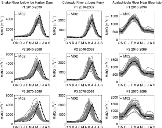
Figure 7.Monthly mean of CMIP5 projected streamflow at three locations indicated in Fig. 5. (left column- Snake River below Ice Harbor Dam, middle column – Colorado River at Lees Ferry, and right column – Apalachicola River near Blountstown). The river routing scheme is KWT. Monthly mean values are computed over three future periods (Top – P1 2010–2039, Middle – P2 2040–2069 and bottom – P3 2070– 2099). The dash line denotes streamflow estimated from runoff output from VIC forced by M02 historical data while gray lines indicate projected streamflow based on future runoff outputs from VIC forced by 28 CMIP5 RCP8.5 data.
In addition, sensitivity of the streamflow estimates to the river routing parameters is examined at selected locations. Different routing model choices (routing scheme and param-eters) will differently affect the attenuation of runoff (i.e., the magnitude of peak and rate of rising and recession limbs) and the timing of the peak flow. We also discuss the effect of dif-ferent river networks (grid-based and vector-based networks) on the results of the runoff routing.
Note that the accuracy of the routed flow is not discussed because it depends largely on the performance of the hydro-logic model that produces the distributed runoff fields and hydrologic model outputs are input to the routing model. The hydrologic simulations can have large errors, which makes a direct comparison with observations less meaningful. For this reason, we focus on an inter-comparison between the two channel routing schemes or two river network definitions. The performance of the IRF-UH approach in routing flows compared to observed flows has been discussed by Lohmann et al. (1996).
5.1 The geospatial fabric network topology
The GF data set was developed primarily to facilitate CONUS-wide hydrologic modeling with the USGS Precipi-tation Runoff Modeling System (PRMS; Leavesley and
grid-Figure 8.Sensitivity of simulated runoff at Colorado River at Lees Ferry (Location B in Fig. 5) to the two KWT parameters. The top panel shows sensitivity to width factorWawith three fixed Manning coefficientsn(from left to right:n=0.005, 0.02, and 0.05). The bottom panel shows sensitivity to Manning coefficientnwith three fixed width factorw(from left to right:Wa=0.0005, 0.0050, and 0.0100).
ded runoff outputs from VIC forced by CMIP-5 data were mapped to each GF HRU by taking the areal-weighted aver-age of the intersecting area between grid boxes and the GF HRUs. Although this paper illustrates runoff routing using GF, the mizuRoute tool can work with any other river net-work data as long as it includes information about the cor-respondence between HRUs and river segments as well as segment-to-segment topology.
5.2 Spatially distributed streamflow in the river network
The first example demonstrates mizuRoute’s capability to produce spatially distributed streamflow estimates over the continental domain. Figure 5 shows daily mean streamflow distribution estimated based on VIC-M02 runoff with KWT and IFR-UH routing methods for 15 June 1986 as an exam-ple. As shown in Fig. 5, both routing schemes produce qual-itatively the same spatial pattern of the daily streamflow.
The mizuRoute tool outputs the time series of the stream-flow estimates at all the river segments in the river network in the NetCDF output file, and modeled streamflow for the point of interest (e.g., streamflow gauge location) can be ex-tracted from the NetCDF based on the ID of the river segment (i.e., seg_id) where the point of interest is located. Figure 6
shows daily streamflow from 1 January 1995 to 31 Decem-ber 1999 extracted at three locations from the NetCDF out-put: (a) Snake River below Ice Harbor Dam, (b) Colorado River at Lees Ferry, and (c) Apalachicola River Blountstown. Temporal patterns of flow simulations with the two river rout-ing schemes are very similar, but the day-to-day differences in estimated streamflow due to the different routing choices become visible.
The next demonstration of mizuRoute’s capability is to produce an ensemble of projected streamflow estimates from the runoff simulations using CMIP5 data. Figure 7 shows the monthly mean of 28 projected streamflow estimates (using CMIP5 RCP 8.5 scenario) extracted at the three locations over three periods: (P1) from 2010 to 2039, (P2) from 2040 to 2069, and (P3) from 2070 to 2099. In this example, the results from the KWT scheme are shown in Fig. 7.
5.3 Sensitivity of streamflow estimates to river routing parameters
Figure 9.Sensitivity of simulated runoff at Colorado River at Lees Ferry (location B in Fig. 5) to IRF-UH parameters. The top panels show sensitivity to diffusivityDwith three fixed celerityCvalues (from left to right:C=1.0, 2.0, and 3.0 ms−1). The bottom panels show
sensitivity to celerityCwith three fixed diffusivityDvalues (from left to right:D=200, 1000, and 3000 ms−2).
parameter values (two parameters for each scheme). We car-ried out the parameter sensitivity analysis at the three loca-tions in Fig. 5, but found the characteristics of the parameter sensitivity are the same at all three. Therefore, we present the results for the Colorado River at Lees Ferry, where a sin-gle, distinct snowmelt runoff peak illustrates the impact of the routing parameter values on the peak timing. Figure 8 shows the effect of the width factorWain Eq. (5) (top panels) and the Manning coefficientn(bottom panels) for the KWT scheme. As expected, wider channels (largerWavalue) delay the hydrograph, because the larger flow area results in slower velocities. This effect is enhanced with larger Manning coef-ficientn, because more friction slows the water flow. A simi-lar effect is seen in the sensitivity experiments for Manning’s n(bottom panel of Fig. 8).
Figure 9 shows the sensitivity of a simulated hydrograph from 1 October 1990 to 30 September 1991 to the two IRF-UH parameters at Colorado River at Lees Ferry (top panel for sensitivity to celerityC and bottom panel for sensitivity to diffusivityD). Interestingly, the effect of diffusivityDis small while celerityC affects the timing of the hydrograph peak. This is because celerityCdirectly changes peak timing without attenuation of IRF, while diffusivityDhas little in-fluence on peak timing of IRF although it changes the degree of flashiness (Eq. 9). Due to the low sensitivity of the
hydro-graph to diffusivityD, the degree of hydrograph sensitivity to celerityC is consistent across different diffusivity values (bottom panel of Fig. 9).
5.4 Comparison between grid-based and vector-based river network
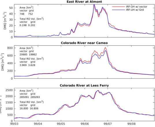
This section illustrates the effect of river network definitions (grid- or vector-based network) on simulated streamflow us-ing the upper Colorado River basin (outlet: Colorado River at Lees Ferry) and two sub-basins (outlets: Colorado River near Cameo and East River near Almont; See Fig. 10). The daily simulated streamflow from March to August 1999 is shown in Fig. 11. The IRF-UH routing scheme in mizuRoute was used to route the VIC-M02 runoff through both GF river network and 1/8◦grid-based river network.
Figure 10.1/8◦(∼12 km) grid-based river network for the upper Colorado River basin(a)and two sub-basins inside the upper Colorado– Colorado River near Cameo and East River at Almont(b). HRUs for each GF river segment are not shown for clarity in(b).
Figure 11.Comparison of IRF-UH routed flow with two river networks (1/8◦grid-based river network and GF vector-based river network)
for sub-basins and total runoff volume that is routed to the gauge as indicated in Fig. 11. Even though the basin areas and therefore flow amounts are similar at Lees Ferry for both networks, they differ for the two sub-basins. For example, the simulated streamflow at Colorado River near Cameo is larger for the vector-based network than for the grid-based network (middle panel in Fig. 11) because of a mismatch in drainage area (Fig. 10). The vector-based river network pre-serves a more accurate drainage shape or area for sub-basins than the 1/8◦grid-based network.
6 Summary and discussion
This paper presents mizuRoute (version 1.0), a river network routing tool that post-processes runoff outputs from any hy-drologic or land surface model. We demonstrated the capa-bility of mizuRoute to produce multi-decadal, spatially dis-tributed streamflow on a vector-based river network using the USGS GF river network over the CONUS. The stream-flow time series are easily extracted at any locations in the network, facilitating hydrologic modeling evaluation, and other hydrologic assessments. The tool is independent of the hydrologic simulations, making it possible to produce ensembles of streamflow estimations from multiple hydro-logic models. As an example of a practical application of mizuRoute, an ensemble of streamflow projections was pro-duced at USGS gauge points on the river systems across the CONUS from 97 runoff simulations from Downscaled CMIP5 Climate and Hydrology Projections (Reclamation, 2014). Section 5.2 shows some of the streamflow simulations based on the runoff generated with VIC forced by CMIP5 data.
Based on the simulations presented in the Sect. 5.3, the routing parameters can affect the simulated hydrograph es-pecially for the KWT method. Though more detailed investi-gations of those effects need to be performed to fully under-stand the routing model behaviors, the parameter sensitivity is substantial. More sophisticated methods to estimate rout-ing model parameters need to be developed. River physical parameters are difficult to obtain in a consistent way at the continental scale, but recent developments of the retrieval al-gorithms for river physical properties (channel width, slope etc.) with remote sensing data are promising (e.g., Pavelsky and Smith, 2008; Fisher et al., 2013; Allen and Pavelsky, 2015), and we expect to see advances in capabilities to esti-mate the hydraulic geometry of rivers over the coming years (Clark et al., 2015).
One limitation of mizuRoute is that the channel routing schemes – KWT and IRF-UH – are both 1-D approaches that do not explicitly track physical parcels of water. The 1-D approach does not allow for explicit modeling of inunda-tion extent, which can occur during flood events. Also, the wave particles that are used in the KWT approach travel at the speed of the wave (celerity) rather than the mean velocity
of the fluid. Therefore, direct use of KWT for water quality modeling such as stream temperature is not recommended. Extension of mizuRoute to simulate stream temperature and water quality can be done in one of two ways: adaptation of the existing routing methods or inclusion of an additional routing scheme that is more directly suitable for tracking wa-ter masses and their constituents.
Toward future enhancements of mizuRoute performance, both routing schemes lend themselves well for paralleliza-tion. Computing speed can be improved by implementing parallel processing directive (e.g., open MP) for routing rou-tines. While kinematic wave routing has to be done sequen-tially from upstream to downstream, the processing can be parallelized through appropriate choices of the domain de-composition. For example, sub-basins that contribute to flow along a mainsteam segment can be processed in parallel be-cause the basins are independent. On a CONUS-wide river network, individual river basins (e.g., the Colorado River and Mississippi River basins) can be processed simultaneously. For IRF-UH routing, the routing computation is performed for individual river segments independently (see Sect. 3.2.2); therefore, the parallelization for river segment loops can be made possible. Lastly, routing of an ensemble of runoff out-puts such as the CMIP5 projected runoff is easily paral-lelized.
7 Code availability
Appendix A: Derivation of wave celerity equation used in KWT
The kinematic wave approximation to the full Saint-Venant equations (Eqs. 3 and 4) uses the continuity equation com-bined with a simplified momentum equation. The simplified momentum equation is based on the assumption that the fric-tion slope is equal to the channel slope and that flow is steady and uniform. Under this assumption, Eq. (4) is reduced to S0=Sf. In other words, the gravitational force that moves water downstream is balanced with the frictional force acting on the riverbed. With this assumption, the dischargeqcan be expressed using a uniform flow formula such as Manning’s equation:
q=Ak nR
α hS
1/2
0 , (A1)
wherekis a scalar, whose value is 1 for SI units and 1.49 for Imperial units,nis the Manning coefficient,Rhis hydraulic radius [L], which is defined as the cross sectional flow area A [L2] divided by the wetted perimeter P [L], and α is a constant coefficient (α=2/3).
We assume the channel shape is rectangular and the ge-ometry is constant throughout one river segment, with width w,A=wy, andP =w+2y. Assuming the channel is wide compared to flow depth (i.e., w≫y), the hydraulic radius Rhis expressed as
Rh= A
P =
wy
w+2y ∼=y. (A2)
By substituting Eq. (A2) into Eq. (A1), the Manning equa-tion is re-written as
q=wk ny
α+1S1/2
0 . (A3)
For each stream segment within which the channel width wis constant, the wave celerityCis given by
C= dq dA=
dq d(wy)∼=
dq
wdy. (A4)
By substituting Manning’s equation (Eq. A3) into Eq. (A4), the wave celerityCcan be given by
C=(α+1)·k n
p
S0·yα (A5)
or expressed as a function of dischargeqas
C=(α+1)·(w)α−+α1 ·
k
n p
S0 α1+1
·qα+α1. (A6)
Appendix B: Derivation of 1-D diffusive equation We describe in detail the derivation of diffusive wave equa-tions from Saint-Venant equaequa-tions (Strum, 2001) that are the
basis of the UH method. The development of the IRF-UH method starts with the derivation of the diffusive wave equation from the 1-D Saint Venant equations (Eqs. 3 and 4) by neglecting inertia terms (the second term in Eq. (4) and assuming steady flow (eliminating the first term in Eq. 4). The momentum equation (Eq. 4) can therefore be reduced to ∂y
∂s =S0−Sf. (B1)
Now, Manning’s equation can be expressed in terms of channel conveyance,Kc(carrying capacity of river channel), q=Kc·
p
Sf, (B2)
whereKc=k/n·A·Rhα. SubstitutingSffrom Eq. (B2) into Eq. (B1) and differentiating with respect to time, the momen-tum equation (Eq. A1) becomes
2q K2 c
∂q ∂t −
2q2 K3 c
∂Kc ∂t = −
∂2y
∂x∂t. (B3)
Also, the continuity equation (Eq. 3) can be re-rewritten by differentiating both sides of the equation with respect to distancexas,
∂2q ∂x2+w
∂2y
∂x∂t =0 (B4)
Combining Eqs. (B3) and (B4) results in 2q
K2 c
∂q ∂t −
2q2 K3 c ∂Kc ∂t = 1 w
∂2q
∂x2. (B5)
Because the channel conveyance,Kc, is a function of flow depth,y, or flow area,A, the differentiation part of the second term of Eq. (B5) can be written as
∂Kc ∂t =
dKc dA
∂A ∂t = −
dKc dA
∂q
∂x. (B6)
Finally, inserting Eq. (B6) into Eq. (B5), results in the one-dimensional diffusive wave equation
∂q ∂t =D
∂2q ∂x2−C
∂q
∂x, (B7)
where C= q
Kc dKc
dA = dq dA
D= K
2 c 2qw =
q 2wS0
, (B8)
Acknowledgements. This work was financially supported by the U.S Army Corps of Engineers Climate Preparedness and Resilience Program.
Edited by: D. Roche
References
Allen, G. H. and Pavelsky, T. M.: Patterns of river width and surface area revealed by the satellite-derived North American River Width data set, Geophys. Res. Lett., 42, 2014GL062764, doi:10.1002/2014gl062764, 2015.
Arora, V. K. and Boer, G. J.: A variable velocity flow routing algo-rithm for GCMs, J. Geophys. Res.-Atmos., 104, 30965–30979, 1999.
Bhunya, P. K., Berndtsson, R., Ojha, C. S. P., and Mishra, S. K.: Suitability of Gamma, Chi-square, Weibull, and Beta distribu-tions as synthetic unit hydrographs, J. Hydrol., 334, 28–38, 2007. Booker, D. J.: Predicting wetted width in any river at any discharge, Earth Surf. Process. Landf., 35, 828–841, doi:10.1002/esp.1981, 2010.
Brunner, G. W.: HEC-RAS, River Analysis Ssytem Users’Manual, US Army Corps of Engineers, Hydrologic Engineering Center, 320, 2001.
Clark, M. P., Rupp, D. E., Woods, R. A., Zheng, X., Ibbitt, R. P., Slater, A. G., Schmidt, J., and Uddstrom, M. J.: Hydrological data assimilation with the ensemble Kalman filter: Use of stream-flow observations to update states in a distributed hydrological model, Adv. Water Res., 31, 1309–1324, 2008.
Clark, M. P., Fan, Y., Lawrence, D. M., Adam, J. C., Bolster, D., Gochis, D. J., Hooper, R. P., Kumar, M., Leung, L. R., Mackay, D. S., Maxwell, R. M., Shen, C., Swenson, S. C., and Zeng, X.: Improving the representation of hydrologic processes in Earth System Models, Water Resour. Res., 51, 5929–5956, doi:10.1002/2015WR017096, 2015.
David, C. H., Maidment, D. R., Niu, G.-Y., Yang, Z.-L., Habets, F., and Eijkhout, V.: River Network Routing on the NHDPlus Dataset, J. Hydrometeorol., 12, 913–934, 2011.
Davies, H. N. and Bell, V. A.: Assessment of methods for extracting low-resolution river networks from high-resolution digital data, Hydrol. Sci. J., 54, 17–28, 2009.
Fekete, B. M., Vörösmarty, C. J., and Lammers, R. B.: Scaling gridded river networks for macroscale hydrology: Development, analysis, and control of error, Water Resour. Res., 37, 1955– 1967, 2001.
Fisher, G. B., Bookhagen, B., and Amos, C. B.: Channel planform geometry and slopes from freely available high-spatial resolution imagery and DEM fusion: Implications for channel width scal-ings, erosion proxies, and fluvial signatures in tectonically active landscapes, Geomorphology, 194, 46–56, 2013.
Gochis, D. J., Yu, W., and Yates, D. N.: The WRF-Hydro model technical description and user’s guide, version 3.0. NCAR Tech-nical Document, NCAR, 120 pp., Boulder CO, 2015.
Goring, D. G.: Kinematic shocks and monoclinal waves in the Waimakariri, a steep, braided, gravel-bed river, Proceedings of the International Symposium on waves: Physical and numerical modelling, University of British Columbia, Vancouver, Canada, 336–345, 1994.
Goteti, G., Famiglietti, J. S., and Asante, K.: A Catchment-Based Hydrologic and Routing Modeling System with ex-plicit river channels, J. Geophys. Res.-Atmos., 113, D14116, doi:10.1029/2007JD009691, 2008.
Horizon Systems Corporation: NHDPlus Version 1 (NHDPlusV1) User Guide, available at: http://www.horizon-systems.com/ NHDPlus/NHDPlusV1_documentation.php (last access: 19 June 2016), 2010.
Koren, V., Reed, S., Smith, M., Zhang, Z., and Seo, D.-J.: Hydrol-ogy laboratory research modeling system (HL-RMS) of the US national weather service, J. Hydrol., 291, 297–318, 2004. Kumar, R., Chatterjee, C., Singh, R. D., Lohani, A. K., and Kumar,
S.: Runoff estimation for an ungauged catchment using geomor-phological instantaneous unit hydrograph (GIUH) models, Hy-drol. Process., 21, 1829–1840, 2007.
Leavesley, G. H. and Stannard, L. G.: The precipitation-runoff mod-eling system-PRMS. Computer Models of Watershed Hydrology, edited by: Singh, V. P., Water Resouces Publications, 281–310, 1995.
Lehner, B. and Grill, G.: Global river hydrography and network routing: baseline data and new approaches to study the world’s large river systems, Hydrol. Process., 27, 2171–2186, 2013. Li, H., Wigmosta, M. S., Wu, H., Huang, M., Ke, Y., Coleman, A.
M., and Leung, L. R.: A Physically Based Runoff Routing Model for Land Surface and Earth System Models, J. Hydrometeorol., 14, 808–828, 2013.
Liang, X., Lettenmaier, D. P., Wood, E. F., and Burges, S. J.: A simple hydrologically based model of land surface water and en-ergy fluxes for general circulation models, J. Geophys. Res., 99, 14415–14428, 1994.
Lohmann, D., Nolte-Holube, R., and Raschke, E.: A large-scale horizontal routing model to be coupled to land surface parametrization schemes, Tellus A, 48, 708–721, doi:10.3402/tellusa.v48i5.12200, 1996.
Lohmann, D., Raschke, E., Nijssen, B., and Lettenmaier, D. P.: Re-gional scale hydrology: I. Formulation of the VIC-2L model cou-pled to a routing model, Hydrol. Sci. J., 43, 131–141, 1998. Lucas-Picher, P., Arora, V. K., Caya, D., and Laprise, R.:
Imple-mentation of a large-scale variable velocity river flow routing algorithm in the Canadian Regional Climate Model (CRCM), Atmos.-Ocean, 41, 139–153, 2003.
Maurer, E. P., Wood, A. W., Adam, J. C., Lettenmaier, D. P., and Nijssen, B.: A Long-Term Hydrologically Based Dataset of Land Surface Fluxes and States for the Conterminous United States, J. Climate, 15, 3237–3251, 2002.
McDonnell, J. J. and Beven, K.: Debates—The future of hydrolog-ical sciences: A (common) path forward? A call to action aimed at understanding velocities, celerities and residence time distri-butions of the headwater hydrograph, Water Resour. Res., 50, 5342–5350, 2014.
Miguez-Macho, G. and Fan, Y.: The role of groundwater in the Amazon water cycle: 1. Influence on seasonal streamflow, flooding and wetlands, J. Geophys. Res.-Atmos., 117, D15113, doi:10.1029/2012JD017539, 2012.
Nadarajah, S.: Probability models for unit hydrograph derivation, J. Hydrol., 344, 185–189, 2007.
O’Donnell, G., Nijssen, B., and Lettenmaier, D. P.: A simple algorithm for generating streamflow networks for grid-based, macroscale hydrological models, Hydrol. Process., 13, 1269– 1275, 1999.
Olivera, F., Lear, M. S., Famiglietti, J. S., and Asante, K.: Extracting low-resolution river networks from high-resolution digital elevation models, Water Resour. Res., 38, 1231, doi:10.1029/2001WR000726, 2002.
Paiva, R. C. D., Collischonn, W., and Tucci, C. E. M.: Large scale hydrologic and hydrodynamic modeling using limited data and a GIS based approach, J. Hydrol., 406, 170–181, 2011.
Paiva, R. C. D., Buarque, D. C., Collischonn, W., Bonnet, M.-P., Frappart, F., Calmant, S., and Bulhões Mendes, C. A.: Large-scale hydrologic and hydrodynamic modeling of the Amazon River basin, Water Resour. Res., 49, 1226–1243, 2013.
Pavelsky, T. M. and Smith, L. C.: RivWidth: A Software Tool for the Calculation of River Widths From Remotely Sensed Imagery, Geosci. Remote Sens. Lett. IEEE, 5, 70–73, 2008.
Reclamation: Downscaled CMIP3 and CMIP5 Hydrology Pro-jections – Release of Hydrology ProPro-jections, Compari-son with Preceding Information and Summary of User Needs, Technical Memorandum No. 86-68210-2011-01, 110 pp., available at: http://gdo-dcp.ucllnl.org/downscaled_cmip_ projections/techmemo/BCSD5HydrologyMemo.pdf (last access: 19 June 2016), 2014.
Reed, S. M.: Deriving flow directions for coarse-resolution (1– 4 km) gridded hydrologic modeling, Water Resour. Res., 39, 1238, doi:10.1029/2003WR001989, 2003.
Strum, T. W.: Open Channel Hydraulics, 1st Edn., McGraw-Hill, 493 pp., 2001.
Taylor, K. E., Stouffer, R. J., and Meehl, G. A.: An Overview of CMIP5 and the Experiment Design, B. Am. Meteorol. Soc., 93, 485–498, 2011.
Viger, R. J.: Preliminary spatial parameters for PRMS based on the Geospatial Fabric, NLCD2001 and SSURGO, US Geologi-cal Survey, doi:10.5066/F7WM1BF7, 2014.
Wu, H., Kimball, J. S., Mantua, N., and Stanford, J.: Automated up-scaling of river networks for macroscale hydrological modeling, Water Resour. Res., 47, W03517, doi:10.1029/2009WR008871, 2011.
Wu, H., Kimball, J. S., Li, H., Huang, M., Leung, L. R., and Adler, R. F.: A new global river network database for macroscale hydrologic modeling, Water Resour. Res., 48, W09701, doi:10.1029/2012WR012313, 2012.
Xia, Y., Mitchell, K., Ek, M., Cosgrove, B., Sheffield, J., Luo, L., Alonge, C., Wei, H., Meng, J., Livneh, B., Duan, Q., and Lohmann, D.: Continental-scale water and energy flux analy-sis and validation for North American Land Data Assimilation System project phase 2 (NLDAS-2): 2. Validation of model-simulated streamflow, J. Geophys. Res.-Atmos., 117, D03110, doi:10.1029/2011JD016051, 2012.
Yamazaki, D., Oki, T., and Kanae, S.: Deriving a global river net-work map and its sub-grid topographic characteristics from a fine-resolution flow direction map, Hydrol. Earth Syst. Sci., 13, 2241–2251, doi:10.5194/hess-13-2241-2009, 2009.
Yamazaki, D., de Almeida, G. A. M., and Bates, P. D.: Improving computational efficiency in global river models by implementing the local inertial flow equation and a vector-based river network map, Water Resour. Res., 49, 7221–7235, 2013.
Yamazaki, D., Kanae, S., Kim, H., and Oki, T.: A physi-cally based description of floodplain inundation dynamics in a global river routing model, Water Resour. Res., 47, W04501, doi:10.1029/2010WR009726, 2011.
Yucel, I., Onen, A., Yilmaz, K. K., and Gochis, D. J.: Calibration and evaluation of a flood forecasting system: Utility of numerical weather prediction model, data assimilation and satellite-based rainfall, J. Hydrol., 523, 49–66, 2015.
![Figure 2. Visualization of waves. The top panel (a) plots a discharge of the wave [m 3 s − 1 ] against its location (distance [km] from the beginning of the 1st segment) at the beginning of five consecutive daily time steps](https://thumb-eu.123doks.com/thumbv2/123dok_br/18404348.359051/4.918.474.850.101.548/figure-visualization-discharge-location-distance-beginning-beginning-consecutive.webp)