Fano interference and a slight fluctuation of the Majorana hallmark
A. C. Seridonio, E. C. Siqueira, F. A. Dessotti, R. S. Machado, and M. Yoshida
Citation: Journal of Applied Physics 115, 063706 (2014); doi: 10.1063/1.4865503 View online: http://dx.doi.org/10.1063/1.4865503
View Table of Contents: http://scitation.aip.org/content/aip/journal/jap/115/6?ver=pdfcov Published by the AIP Publishing
Articles you may be interested in
Quantum transport through the system of parallel quantum dots with Majorana bound states J. Appl. Phys. 115, 083706 (2014); 10.1063/1.4867040
Identifying Dirac cones in carbon allotropes with square symmetry J. Chem. Phys. 139, 184701 (2013); 10.1063/1.4828861
Tunneling transport through multi-quantum-dot with Majorana bound states J. Appl. Phys. 114, 033703 (2013); 10.1063/1.4813229
Signature of quantum interference and the Fano resonances in the transmission spectrum of bilayer graphene nanostructure
J. Appl. Phys. 110, 014306 (2011); 10.1063/1.3603005
Fano interference and a slight fluctuation of the Majorana hallmark
A. C. Seridonio,1,2E. C. Siqueira,2F. A. Dessotti,2R. S. Machado,2and M. Yoshida11Instituto de Geoci
^
encias e Ci^encias Exatas-IGCE, Universidade Estadual Paulista, Departamento de Fısica, 13506-970, Rio Claro, Sao Paulo, Brazil~
2Departamento de F
ısica e Quımica, Universidade Estadual Paulista, 15385-000, Ilha Solteira, Sao Paulo, Brazil~
(Received 19 December 2013; accepted 31 January 2014; published online 13 February 2014)
According to the Liu and Baranger [Phys. Rev. B 84, 201308(R) (2011)], an isolated Majorana state bound to one edge of a long enough Kitaev chain in the topological phase and connected to a quantum dot, results in a robust transmittance of 1/2 at zero-bias. In this work, we show that the removal of such a hallmark can be achieved by using a metallic surface hosting two adatoms in a scenario where there is a lack of symmetry in the Fano effect, which is feasible by coupling the Kitaev chain to one of these adatoms. Thus in order to detect this feature experimentally, one should apply the following two-stage procedure: (i) first, attached to the adatoms, one has to lock AFM tips in opposite gate voltages (symmetric detuning of the levelsDe) and measure by an STM tip, the zero-bias conductance; (ii) thereafter, the measurement of the conductance is repeated with the gates swapped. For jDej away from the Fermi energy and in the case of strong coupling tip-host, this approach reveals in the transmittance, a persistent dip placed at zero-bias and immune to the aforementioned permutation, but characterized by an amplitude that fluctuates slightly around 1/2. However, in the case of a tip acting as a probe, the adatom decoupled from the Kitaev chain becomes completely inert and no fluctuation is observed. Therefore, the STM tip must be considered in the same footing as the “hostþadatoms” system. As a result, we have found that despite the small difference between these two Majorana dips, the zero-bias transmittance as a function of the symmetric detuning yields two distinct behaviors, in which one of them is unpredictable by the standard Fano’s theory. Therefore, to access such a non trivial pattern of Fano interference, the hypothesis of the STM tip acting as a probe should be discarded.VC 2014 AIP Publishing LLC.
[http://dx.doi.org/10.1063/1.4865503]
I. INTRODUCTION
Majorana fermions are particles that constitute their own antiparticles. Such a proposal was made almost a century ago by Ettore Majorana in the context of high-energy physics. In solid state systems, these exotic particles are not fundamental but emerge as quasiparticle excitations.1This species of exci-tation is ranked as non-Abelian anyons and obeys an unusual quantum statistics. Its most remarkable property lies on the possibility of bounding two far apart Majoranas that define an unique nonlocal Dirac fermion. Once this spatially delocal-ized state is occupied, it yields a robust qubit decoupled from the surroundings, thus avoiding decoherence due to perturba-tions. This protected qubit then enlarges the feasibility to make these blocks as essential to the accomplishment of a topological quantum computer. Thus, in the last few years, the quest for devices nesting Majorana fermions has received much attention from the community of researchers working with quantum computing.2–6
To the best knowledge, the superconductor state is con-sidered suitable for the emergence of Majorana excitations. Superconductivity lies on Cooper-pair condensation and spon-taneous breaking of charge conservation, thus leading to the superposition of electrons and holes. However, s-wave super-conductivity arises from electrons with opposite spins that result in distinct operators for creation and annihilation of qua-siparticles, thus preventing the realization of Majorana bound
states (MBSs). To support them, a spinless superconductor is indeed required. Such conditions can be found in the topologi-cal phase of the Kitaev chain,7which offers the proper envi-ronment to sustain Majoranas. The Majoranas are zero-energy modes, in particular, placed at the edges of this chain.
The engineering of a sample withp-wave superconduc-tivity can be achieved experimentally by proximity effect. It is known that a s-wave superconductor nearby a semicon-ducting nanowire with strong spin-orbit interaction and crossed by a magnetic field, inducesp-wave superconductiv-ity on the latter system.8–16 Additionally, the existence of Majoranas are predicted in the fractional quantum Hall state with filling factor¼5/2,17in three-dimensional topological insulators18and at the core of superconducting vortices.19–21 In this scenario, quantum transport becomes a sensible tool for detecting Majorana quasiparticles. Particularly in Ref.22, it was predicted for the experimental setup of a single quan-tum dot (QD) side-coupled to a Majorana state, that the zero-bias peak (ZBP) for the conductance should be given by the robust Majorana hallmarkG ¼0:5G0, whereG0¼e2=his the
background conductance. We highlight that in Ref. 23, Verneket al. have determined that such an amplitude arises from the leaking of the Majorana state into the QD.
Experimentally, a persistent ZBP has been observed in transport measurements through a setup composed by a nano-wire of indium antimonide merged to gold and niobium tita-nium nitride.24In this aforementioned system, Majoranas are
0021-8979/2014/115(6)/063706/10/$30.00 115, 063706-1 VC2014 AIP Publishing LLC
supposed to exist due to the ZBP that stands up to a wide range of magnetic fields and gate voltages. Such a robustness of the ZBP has also been found in the analogous system of a superconductor of aluminium close to a nanowire of indium arsenide.25Moreover, we stress that the ZBP feature may also have another physical origin, for instance, the Kondo effect.26–33
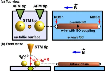
In this context, an apparatus based on Fano effect34,35 becomes an alternative approach to detect a Majorana state. Here, we benefit of this mechanism, an interference phenom-enon found in systems where tunneling channels compete for the electron transport. This effect can be detectable by the Scanning Tunneling Microscope (STM), a device made by a metallic tip that detects, for low enough temperatures, the transmittance through a system by measuring the differential conductance.29–33Thus, we have studied theoretically the con-ductance probed by an STM tip of a metallic surface coupled to two adatoms, in which one of them is coupled to a MBS hosted by a long enough Kitaev chain in the topological phase. We should remark that nowadays such a chain is achievable experimentally as found in Ref. 24, whose system becomes the most promising candidate to our proposal [see Fig.1].
Additionally, we have considered in the model two Atomic Force Microscope (AFM) tips capacitively coupled to the adatoms, just in order to tune their levels as proposed in Ref.36. Our approach employs the spinless Hamiltonian of Ref.22in combination with the equation-of-motion pro-cedure for the Green’s functions.
By determining the transmittance of this setup, we have found Fano profiles due to the coupling between the setup of the adatoms and an isolated MBS. For the setup decoupled from this MBS, the direct and the mixed Green’s functions are symmetric with respect to the labels 1 and 2 that desig-nate the parameters of the adatoms. In the opposite limit, this symmetry property is broken and the swap of the indexes 1$2 leads to a lack of symmetry in the Fano profile.
This lack of symmetry can be accessed experimentally by performing the following proposed two-stage procedure: (i) first, attached to the adatoms, one has to lock AFM tips in opposite gate voltages (symmetric detuning of the levelsDe) and measure by an STM tip, the zero-bias conductance; (ii) thereafter, the measurement of the conductance is repeated with the gates swapped.
As a result of this method and the Fano regime as well, the transmittance forjDejaway from the Fermi energy exhibits a zero-bias dip persistent against the permutation of the gate voltages. For the case in which the STM acts as a probe of the LDOS (local density of states) for the “hostþadatoms” system, the adatom decoupled from the Kitaev chain plays no role and the typical Majorana hallmark is verified: a robust zero-bias transmittance characterized by an amplitude of 1/2 as that found in Ref.22for a single QD setup. On the other hand, for the STM in the same footing as the “hostþadatoms” system, a slight fluctuation around the amplitude of 1/2 manifests as a straight aftermath of the two-stage procedure in combination with the adatom free of the MBS. However, despite the small difference between these two Majorana dips, each one leads to a particular Fano lineshape for the zero-bias transmittance as a function of the symmetric detuning. Therefore, we demon-strate in this work that the assumption of the STM as a probe tip is not enough to reveal the unexpected pattern of Fano in-terference for the proposed setup of Fig.1.
This paper is organized as follows. In Sec.II, we show the theoretical model for the system sketched in Fig. 1 as well as the derivation of the transmittance. The Green’s functions of the adatoms are also presented in this section. The results appear in Sec.IIIand in Sec.IV, we summarize the conclusions.
II. THEORETICAL MODEL
A. Hamiltonian
The system we investigate is described according to the Hamiltonian
Htotal¼ Hhostþadsþ Htipþ Htun: (1)
In order to mimic the system outlined in Fig. 1, we follow the spinless Hamiltonian proposed by Liuet al.,22
taking two adatoms into account, which reads
Hhostþads¼ X
k
ðeklhostÞc † kckþ
X
j ejdj†dj
þV X
jk
c†kdjþH:c:
þiMg1g2
þkðd1d†1Þg1; (2)
where the electrons in the host are described by the operator c†k(ck) for the creation (annihilation) of an electron in a
quan-tum state labeled by the wave numberk, energyekand
chem-ical potential lhost. For the adatoms, dj† (dj) creates
(annihilates) an electron in the stateej, withj¼1, 2.Vis the
hybridization of the adatoms with the host. In particular for j¼1, the adatom 1 is coupled to the MBS 1 described by the operator g†1 ¼g1. The strength of this coupling is k. The
MBS 2 given byg†2¼g2 is connected to the MBS 1 via the
coefficient MeL=n, with L being the distance between the MBSs andnthe coherence length. It is worth mentioning that the present spinless model supposes a strong magnetic field over the entire system, which leads to a large Zeeman splitting where the higher levels are not energetic favorable at low temperatures. In this situation, one spin component plays no role and the spin degrees of freedom can be ignored.
The second part of Eq. (1) is described by the Hamiltonian
Htip¼ X
q
ðeqltipÞb †
qbq; (3)
which corresponds to free electrons ruled by fermionic oper-atorsb†
qandbqin the STM tip, with energyeqand chemical
potentialltip.
To perform the coupling between Eqs. (2) and(3), we have to define the tunneling Hamiltonian
Htun ¼wðft†w0þH:c:Þ; (4)
wherewis the STM tip-host coupling,
ft¼
X
q
bq (5)
is for the edge of the STM tip,
w0¼f0þ ðpCq0Þ 1=2
q0 X
j
dj (6)
is the field operator that accounts for Fano interference,
f0¼ X
k
ck (7)
represents the host site laterally coupled to the adatoms [see the green-circle of the host outlined in Fig.1],
C¼pV2q0 (8)
is the Anderson parameter, with q0 ¼21D as the density of states for the surface without adatoms, D is the band half-width and
q0¼ ðpCq0Þ 1=2 V~
w
(9)
is the Fano factor of interference,37withV~as the couplings between the STM tip and the adatoms. Notice that due to Eqs.(6) and(9), the limitq01 represents the situation in
which the tip is highly hybridized with the adatoms, while in the opposite regime q0¼0, the tip is strongly connected to the surface [see Fig.1]. As the former case in presence of a MBS still obeys the standard Fano’s theory, in this work we will focus on the latter, where we can find a non trivial Fano interference. Such a point will be discussed in Sec.III.
B. Calculation of the transmittance
1. The STM tip as a probe
By applying the linear response theory, in which the STM tip is considered as a probe, it is possible to show that the zero-bias conductance is given by
Gð0Þ ¼e
2
hð2pwÞ
2ð
qLDOSðeÞqtipðeÞ
@fF @e
de; (10)
where e is the electron charge, h is the Planck constant, qLDOS (e) is the LDOS of the “hostþadatoms” system, qtip (e) as the DOS of the STM tip andfFis the Fermi-Dirac
dis-tribution. The total transmittance is then defined as follows:
TprobeðeÞ ¼ ð2pwÞ2qLDOSðeÞqtipðeÞ: (11)
To obtain the LDOS, we follow Ref. 36by introducing the retarded Green’s function
Rw0w0¼
i
hhð Þt Tr .hostþads½w0ð Þt ;w
† 0ð Þ0 þ
n o
(12)
for the field operator of Eq. (6)in the time domaint, where h(t) is the Heaviside function,.hostþads is the density matrix of the system described by the Hamiltonian in Eq. (2) and
½ ; þ is the anticommutator of Eq.(6)at distinct times. From Eq.(12), the LDOS of the host can be obtained as
qLDOSðeÞ ¼
1
pImðR~w0w0Þ; (13)
whereR~w0w0is the Fourier transform ofRw0w0 in the energy
domaine. Analogously, we have
qtipðeÞ ¼
1
pImðR~ftftÞ; (14)
with
Rftft ¼
i
hhð Þt Tr .tip½ftð Þt ;f
† tð Þ0 þ
n o
; (15)
where .tip is the density matrix of the system described by
the Hamiltonian in Eq.(3).
Thus to determine an analytical expression for the LDOS, we apply the equation-of-motion approach on Eq.
(12). Such a procedure is summarized as follows:
ðeþigÞR~AB¼ ½A;B†
þþR~½A;HiB; (16)
withg!0þ,AandBas fermionic operators belonging to the HamiltonianHi(i¼hostþads or tip).
By taking Eq. (12), one can calculate via Eqs. (2), (6), and(16)withA ¼ B ¼w0andHi¼ Hhostþads, the following
relation:
~
Rw0w0 ¼R~f0f0þ ðpCq0Þq 2 0
X
jl
~
Rdjdlþ2ðpCq0Þ 1=2
q0
X
j
~
Rdjf0; (17)
which depends on the Green’s functions R~f0f0;R~f0dj and
~
Rdjdl. First, we findR~f0f0,
~
Rf0f0¼pq0ðciÞ þpq0CðciÞ 2X
jl
~
Rdjdl (18)
and later on, the mixed Green’s functionR~djf0,
~ Rdjf0¼
ffiffiffiffiffiffiffiffiffiffiffi
pCq0 p
ðciÞX l
~
Rdjdl; (19)
where
c¼ 1
pq0 X
k 1 eek
: (20)
Now, we choose for Eq. (16), Hi¼ Htip and A ¼ B ¼ft, respectively, from Eqs.(3)and(14), to show that
~
Rftft ¼pq0ðciÞ: (21)
In particular, for the wide band limit D! 1,c!0. Thus, the imaginary parts of Eqs.(18)–(21)become
ImðR~f0f0Þ ¼ pq0½1þC X
jl
ImðR~djdlÞ; (22)
ImðR~djf0Þ ¼ ffiffiffiffiffiffiffiffiffiffiffi
pCq0 p X
l
ReðR~djdlÞ (23)
and
ImðR~ftftÞ ¼ pq0: (24)
Now, we take Eqs.(22)–(24)into Eq.(11)to obtain
TprobeðeÞ ¼T probeðeÞ
Tb ¼
1þCX jl
½ð1q20ÞImðR~djdlÞ
þ2q0ReðR~djdlÞ (25)
as the total transmittance through the system, expressed in terms of the background conductance
Tb¼4x¼4ðpwq0Þ 2
; (26)
and the Green’s functionsR~djdlof the adatoms.
2. The STM tip in the same footing as the “host1adatoms” system
Here, we derive the Landauer-B€uttiker formula for the zero-bias conductance Gð0Þ by considering the STM tip in
the same footing as the “hostþadatoms” system, which is achievable withV~¼Vin Eq.(9).
The zero-bias conductance is a function of the transmit-tanceTfullð Þe as follows:
Gð0Þ ¼@@
uJhostðu¼0Þ ¼ e2
h
ð
de @fF @e
TfullðeÞ; (27)
with Jhost as the current for the host and lhostltip¼eu,
with u as the applied bias-voltage. We begin with the transformation ck bk ¼ 1 ffiffiffi 2
p 1ffiffiffi
2
p
1ffiffiffi
2
p 1ffiffiffi
2 p 0 B B B @ 1 C C C A cok cek ; (28)
on the Hamiltonian of Eq. (1), which depends on the even and odd conduction operators cek and cok, respectively.
These definitions allow us to express Eq.(1)as
H ¼ Heþ HoþH~tun¼ Hu¼0þH~tun; (29)
where
He¼
X
k
ekc†ekcekþ
X
j ejd†jdj
þX
jk
ffiffiffi
2
p
Vðc†ekdjþH:c:Þ þw
X
kq c†ekceq
þiMg1g2þkðd1d†1Þg1 (30)
represents the Hamiltonian part of the system coupled to the adatoms via an effective hybridizationpffiffiffi2V, while
Ho¼
X
k
ekc†okcokw
X
kq
c†okcoq (31)
is the decoupled one. However, they are connected to each other by the tunneling Hamiltonian
~
Htun ¼ Dl X
k
ðc†ekcokþc†okcekÞ; (32)
with lhost¼Dl;ltip¼ Dl and Dl¼eu=2. As in the
zero-bias regimeDl!0, due tou!0;H~tun is a
perturba-tive term.
Here, we use the interaction picture to calculateTfullðeÞ.
It ensures that a state jUni from the spectrum of the Hamiltonian given by Eq. (29) admits the following time-dependency:
jUni ¼eih Ð0
1H~tunðsÞdsjWni
’ 1i
h
ð0
1
~ HtunðsÞds
!
jWni; (33)
whereh¼ h
performing the expected mean value of the current operator
Ihost Ihostðt¼0Þ, which reads
Jhost ¼ hUnjIhostjUni
¼ i
h Wn
ð0
1½I
host;H~tunðsÞds Wn
þ OðH~2tunÞ;
(34)
where we have regardedhWnjIhostjWni ¼0 and by
consider-ing the thermal average on the latter equation, which gives
Jhost ¼
i
h
ð0
1
Tr .u¼0½Ihost;H~tunðsÞ
n o
ds; (35)
where.u¼0is the density matrix of the system described by
the HamiltonianHu¼0in Eq.(29). By applying the
equation-of-motion onIhost, we show that
Ihost ¼
i
h½e
X
k
c†kck;Hu¼0
¼ ieffiffiffi
2 p h VX kj
ðc†ekdjd†jcekÞþðc†okdjdj†cokÞ
n o
þ ie
h
wX qq~
ðc†
oqceq~c†e~qcoqÞ; (36)
which, in combination with Eq.(35), leads to
Jhost¼
e
hDlIm
ðþ1
1
ds pffiffiffi2VX j
FjðsÞþ2wMðsÞ
;
(37)
where
FjðsÞ ¼ i
hhðsÞTr .u¼0½f
† odj;
X
q c†
eqðsÞcoqðsÞ
(38)
and
MðsÞ ¼ i
hhðsÞTr .u¼0½f
† ofe;
X
k
c†ekðsÞcokðsÞ
(39)
are retarded Green’s functions, expressed in terms of the operators
fo¼
X
~ q
coq~ (40)
and
fe¼
X
q
ceq: (41)
In order to find a closed expression for the currentJhost,
we should evaluate the integrals in the time coordinatesof Eq.(37), which result in
ðþ1
1
dsFjðsÞ ¼ Z1
X
mn
ðebEnebEmÞ
EnEmþig
hWnjfo†djjWmihWmj
X
q
c†eqcoqjWni
(42)
and
ðþ1
1
dsMðsÞ ¼ Z1X
mn
ðebEnebEmÞ
EnEmþig
hWnjfo†fejWmi
D
Wm
X
q c†eqcoq
Wn E ; (43)
where we have used Z as the partition function of
Hu¼0jWmi ¼EmjWmi,Að Þ ¼s e
i
hHu¼0sAehiHu¼0s for an
arbi-trary time-dependent operatorAð Þs andg! 0þ. To elimi-nate the matrix element hWmjc†
eqcoqjWni in Eqs. (42) and
(43), we calculatehWmj½P
qc†eqcoq;Hu¼0jWni, which gives
D
Wm
X
q c†eqcoq
Wn E ¼ ffiffiffi 2 p V
ðEnEmÞ
X
~ j
hWmjd†~ jfojWni
2w
ðEnEmÞhWmj
fe†fojWni: (44)
By performing the substitutions of Eqs.(42),(43) with
(44) in Eq.(37), we enclose the result into the function la-beled byvmnto show that
Jhost ¼
e
hpDlZ 1X
mn vmnðe
bEnebEmÞ
EnEm
dðEnEmÞ
¼ e
hpDlb
X
mn
½Z1ebEndðE
nEmÞvnm; (45)
where we have defined
vnm¼ ðpffiffiffi2VÞ2X j~j
hWnjfo†djjWmihWmjd†~jfojWni
þ2pffiffiffi2Vð2wÞX
j
hWnjfo†djjWmihWmjfe†fojWni
þð2wÞ2hWnjfo†fejWmihWmjfe†fojWni: (46)
In this calculation, we have used
hWnjf†
odjjWmihWmjfe†fojWni
¼ hWnjf†
ofejWmihWmjdj†fojWni;
with
ðebEnebEmÞ
EnEm ¼
bebEn (47)
in the limitEn!Em. The property½He;Ho ¼0 ensures the partitionsEn¼EenþEonandZ ¼ ZeZofor the Hamiltonians
He and Ho, respectively in the brackets of Eq. (45), thus leading to
Z1ebEndðE
nEmÞ ¼ 1 bZ 1 e Z 1 o ð
de @fF @e
ðebEenþebEemÞðebEonþebEomÞ
dðeþEenEemÞdðeþEonEomÞ: (48)
Therefore, we substitute Eqs. (46)and(48)in Eq.(45)
to calculate@@uJhostðu¼0Þ. The comparison of such a result
with Eq.(27)allows us to find
Tfullð Þ ¼ ðe 2pwÞ 2
~
qLDOSðeÞ~qtipðeÞ; (49)
where
~
qLDOSðeÞ ¼
1
pImðR~weweÞ (50)
and
Rwewe ¼
i
hhð Þt Tr .e½weð Þt ;w
† eð Þ0 þ
n o
; (51)
with the former as the renormalized LDOS of the “hostþadatoms” system described by the Hamiltonian of Eq.
(30), which is affected by the STM tip via the scattering term wP
kqc †
ekceq, thus leading to
we¼feþ ðpDq0Þ 1=2
cX j
dj (52)
and
~
Rwewe ¼R~fefeþ ðpq0DÞc 2X
jl
~ Rdjdl
þ2ðpq0DÞ 1=2
cX j
~ Rdjfe
that generalize Eqs.(6)and(17), respectively, with a renor-malized Anderson parameter
D¼2pV2q0 (53)
and Fano factor
c¼ðpq0DÞ 1=2
ffiffiffi 2 p V 2w : (54)
Additionally, the scattering termwP
kqc †
okcoq renorm-alizes the DOS of the STM tip due to the Hamiltonian of Eq.
(31), which provides
~
qtipðeÞ ¼
1
pImðR~fofoÞ: (55)
From Eqs. (30) and (41), we make the substitutions
A ¼ B ¼feandHi¼ Hein Eq.(16), which gives
~ Rfefe ¼
pq0ðciÞ
1 ffiffiffi
x
p
ðciÞþpq0D
ðciÞ
1 ffiffiffi
x
p ðciÞ
2
X
jl
~
Rdjdlð Þe; (56)
where we have used the mixed Green’s function
~ Rdjfe ¼
ffiffiffiffiffiffiffiffiffiffiffi
pDq0
p ðciÞ
1 ffiffiffi
x
p ðciÞ
X
l
~
Rdjdl; (57)
determined from Eq.(16)by consideringA ¼dj;B ¼feand
Hi¼ He, with the parameter xbeing the same as found in Eq. (26). We point out that, Eqs. (56) and (57) constitute respectively, generalizations of Eqs.(18)and(19), where the latter can be obtained from the former by making x 1. Thus, the imaginary parts of Eqs. (56)and(57)for the wide band limitD!1, become
ImðR~fefeÞ ¼
pq0
1þx
ð1xÞ ð1þxÞ2pDq0
X
jl
ImðR~djdlÞ
þ 2
ffiffiffi
x
p
1þx
ð Þ2pDq0
X
jl
ReðR~djdlÞ (58)
and
ImðR~djfeÞ ¼
ffiffiffiffiffiffiffiffiffiffiffiffiffi
xpDq0 p
1þx
X
l
ImðR~djdlÞ
ffiffiffiffiffiffiffiffiffiffiffi
pDq0 p
1þx
X
l
ReðR~djdlÞ; (59)
where we have used c!0. To conclude, we notice that
~
Rfofo is decoupled from the adatoms. Thereby, from Eqs.
(31)and(40), we takeA ¼ B ¼fo andHi¼ Hoin Eq.(16) and we obtain
ImðR~fofoÞ ¼
pq0
1þx; (60)
which is equal to the first term of Eq.(58).
Thus the substitution of Eqs.(58)–(60)in Eq.(49), leads to
TfullðeÞ ¼T fullðeÞ
Tb ¼
1þCX jl
½ð1q2
bÞImðR~djdlÞ
þ2qbReðR~djdlÞ; (61)
where
Tb ¼
4x
1þx
ð Þ2 (62)
represents the transmittance in the absence of the adatoms and MBSs (background contribution),
C¼ D
is an effective coupling and
qb¼ 1x
ð Þ
2pffiffiffix (64)
is the Fano parameter. Notice that Eq. (61) has the same form of Eq.(25), but withq0replaced byqb. In this work, we
will focus on the limitq0¼qb¼0.
C. Green’s functions of the adatoms
In this section, we calculate the Green’s functionsR~djdl
within the wide band limitD ! 1. We point out that, the expressions derived here describe the situation of Sec.II B 1
for an STM tip as probe withC instead ofD [see Eqs. (8)
and(53)] and by assumingx 1 [Eq.(26)], otherwise, they belong to the case of Sec.II B 2. We begin by applying the equation-of-motion procedure on
Rdjdl¼
i
hhð Þt Tr .s½djð Þt ;d
† lð Þ0 þ
n o
; (65)
where s¼hostþads or s¼e, and changing to the energy do-maine, we obtain the following relation:
ðe~ejiRIdj1RMBS1ÞR~djdl ¼djlþR X
~ l6¼j
~
Rd~ldl; (66)
with
~
ej¼ejþRR (67)
is the adatom level renormalized by the STM tip-host cou-plingw, withR¼RRþiRI,
RR¼
ffiffiffi
x
p
1þxD; (68)
RI ¼ D
1þx (69)
and
RMBS1¼k2Kð1þk2K~Þ (70)
as the self-energy due to the MBS 1 coupled to the adatom 1,
K¼1
2
1 eMþigþ
1 eþMþig
(71)
and
~
K ¼ K
eþ~e1iRIk2K
; (72)
which have the same forms as found in Ref.22. Thus, the so-lution of Eq.(66)provides
~ Rd1d1 ¼
1
e~e1iRIRMBS1 C2
(73)
as the Green’s function of the adatom 1, with
Cj¼ðR Rþi
RIÞ2
e~ejiRI
; (74)
as the self-energy due to the presence of thejthadatom. For
C2¼0, we highlight that Eq.(73)is reduced to the Green’s
function of the single QD system found in Ref. 22. In the case of the adatom 2, we have
~ Rd2d2 ¼
1R~0d1d1RMBS1
e~e2iRI
~ R0d1d1
~ R0d2d2
RMBS1 C1
; (75)
where R~0d1d1¼1=ðe~e1iR
IÞ and R~0
d2d2¼1=ðe~e2iR IÞ
represent the corresponding Green’s functions for the single adatom system without Majoranas. To conclude, the mixed Green’s functions are
~ Rd2d1¼
RRþiRI e~e2iRI
~
Rd1d1 (76)
and
~ Rd1d2¼
RRþiRI e~e1iRIRMBS1
~
Rd2d2: (77)
The main result of this section is the emergence of a lack of symmetry in these Green’s functions. This property lies on the coupling of the adatom 1 with the MBS 1. To notice that, let us examine the situation where the adatom 1 is decoupled from the MBS 1, which can be obtained with RMBS1¼0 in Eq. (70). By inspection of Eqs. (73) and
(75)–(77), we verify that the functions R~d1d1 andR~d1d2 can
be determined by the swap of the indexes 1 $ 2 in R~d2d2
and R~d2d1, respectively. However, in the opposite situation
with RMBS16¼0, this symmetry is broken. Thus, in Sec. III, we will investigate this lack of symmetry via the transmittan-ces of Eqs. (25) and (61). To this end, we will follow the two-stage procedure presented in Sec.I.
III. RESULTS
Here, we consider the Kitaev chain long enough, which forcesMeL=n!0 in Eq.(2)forLn. We adopt typical values for adatoms in metals [Ref. 32]: D¼C¼0.2 for the Anderson parameters of Eqs. (8) and (53), k, e1¼ D2e;
e2¼D2e, the symmetric detuning De¼e2e1 ande in units
of eV.
In order to investigate the transmittanceTfull(e) of Eq.
(61)as a function of the single particle energye, in Fig.2we use k¼5D, with x¼1 and Fano factor qb¼0 [Eq. (64)].
This set of parameters allows one to emulate the situation where the STM tip is strongly connected to the host surface and therefore, considered in the same footing as the “hostþ
adatoms” system.
In Fig.2(a) for the case of a free system, i.e., without MBSs [solid-green curve], we observe two antiresonances, each one placed around the corresponding adatom level given by e1¼ 2.5 and e2¼ þ2.5, respectively. We name
these antiresonances as satellite dips. Off the antiresonances, the transmittance approaches the unitary limit and the con-ductance reaches G ¼ G0¼e2=h. Notice, for instance, the
central region bounded by the range 1:75ⱗeuⱗ1:5 [shaded region], where we have a ballistic plateau with the aforementioned conductance. In this free system, the Green’s functions of the model are symmetric under the per-mutation of the indexes that designate the parameters of the adatoms. This property is confirmed by the corresponding solid-green curve of Fig.2(b), obtained with e1¼ þ2.5 and e2¼ 2.5, which agrees with that for e1¼ 2.5 and e2¼ þ2.5 in Fig. 2(a). Therefore, the two-stage procedure proposed in this work, in particular for the case of a free dou-ble adatom system, yields two identical curves for the trans-mittance. However, for the device side-coupled to the MBS 1, a novel feature emerges in the central region.
By fixing e1¼ 2.5 and e2¼ þ2.5, a dip of amplitude nearby 1/2 arises in the middle of the ballistic plateau, due to the MBS 1 attached to the adatom 1 [see the dashed-blue curve in Fig. 2(a)]. For this situation, the dip around e2¼ þ2.5 coincides with the corresponding one found in the
solid-green curve of the free setup, which is due to the adatom 2 decoupled from the MBS 1. Moreover, the antiresonance in the vicinity of e1¼ 2.5 is not coincident with that in Fig.
2(a) of the solid-green curve for the free system. As we can see, the position of such an antiresonance is shifted as the aftermath of the coupling between the MBS 1 and the adatom 1. After the swap procedure, which leads to e1¼ þ2.5 and e2¼ 2.5, the satellite dips of Fig. 2(b)[see the dashed-red lineshape] become reversed with respect to those found in Fig.2(a).
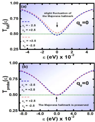
We emphasize that the central antiresonance remains placed at zero-bias, but its amplitude fluctuates slightly around 1/2. This behavior of the central dip appears in Fig.
3(a), which can be clearly visualized in the dashed-blue and red lineshapes, respectively. Therefore, a pinned antireso-nance protected against the two-stage procedure emerges in the transmittance, which is placed at the zero-bias and char-acterized by an amplitude nearby 1/2. In contrast, the satel-lite dips do not share such a pinning, since they move significantly under the permutation of the levels in the ada-toms. However, the complete robustness of the Majorana hallmark does not exist anymore as found in Refs. 22 and
23: the amplitude is not fixed at 1/2 as a straight result of the interplay between the adatom decoupled from the Kitaev
FIG. 2. Parameters employed:M¼0 [long enough Kitaev chain],k¼5D andD¼0.2 [see Eqs.(2)and(53)]. TransmittanceTfull(e) determined by Eq.(61)in the Fano regimeqb¼0 [Eq.(64)] as a function of the single par-ticle energye. In the panels (a) and (b) we have: the solid-green lineshape is for the apparatus of Fig.1in the absence of the MBS 1. Implementation of the two-stage procedure of Sec. I: (a) e1¼ 2.5 and e2¼ þ2.5: The dashed-blue curve corresponds to the system coupled to the MBS 1. (b)
e1¼ þ2.5 ande2¼ 2.5: The dashed-red lineshape is for the MBS 1. Here we see the main result of this procedure: the formation of a Majorana dip with an amplitude that fluctuates slightly around 1/2, but it remains pinned at zero-bias even by performing the gates swap. The satellite dips do not share such a feature, they become significantly shifted under the permutation of the levels in the adatoms.
chain and the Fano regime as well, obtained with x¼1 in Eq.(64). In this situation, the real and imaginary parts of the self-energyR, which readRRandRI, respectively, given by Eqs.(68)and(69), depend onx. Otherwise, it would corre-spond to the case of the tip considered as a probe of the LDOS for the “hostþadatoms” system, which suppresses the fluctuation of the Majorana hallmark. This feature can be observed by using the transmittance Tprobe (e) of Eq. (25)
withq0¼0, which is confirmed by the dashed-blue and red lineshapes of Fig.3(b). In fact, it can be observed an antire-sonance pinned at zero-bias characterized by a constant am-plitude of 1/2. In this case,RR andRIdo not depend on x, sincex 1 for a probe tip [see Eq.(26)]. As a result, the Majorana hallmark is preserved under the gates swap.
Thus in order to explore the effects due to the fluctuation of the zero-bias transmittance, we present the analysis of Tfull(0) andTprobe(0) as a function of the symmetric detun-ing De. In both cases, the Fano parameters are qb¼0 and
q0¼0, which according to Fano’s theory, lead to a destruc-tive interference pattern. Such a behavior can be seen in the transmittance versus e plots of Figs. 3(a) and 3(b). Additionally, we point out that the Majorana dip verified in
the former differs slightly with respect to that found in the latter. Remarkably, the slight fluctuation of the Majorana hallmark in Fig.3(a)is able to provide an unexpected profile of Tfull(0) versus De, which differs expressively of a Fano dip. The result of this analysis appears in the solid-violet curve of Fig.4(a), where it is observed that the transmittance approaches 1/2 from upper (lower) values for De<0 (De>0). In the domain ofDe<0, it reaches the maximum value of 3/4, while forDe>0, it decreases to 1/4. Notice that the variation of the transmittance withDedoes not exceed an amplitude of 1/2 and particularly atDe¼0, the transmittance recovers the Majorana hallmark 1/2. On the other hand, in Fig.4(b), the transmittance Tprobe(0) as a function ofDein the solid-orange curve, displays the standard profile of Fano antiresonance for q0¼0. Notice that in both Figs. 4(a) and
4(b), the variation of the transmittance with De is 1/2. We highlight that the unexpected Fano profile found in this work becomes a way to identify the existence of isolated MBSs, since the lineshape in Fig. 4(a) is due to a long enough Kitaev chain within the topological phase.
In summary, despite the same Fano parametersq0¼0 and qb¼0 inTprobe (0) andTfull(0), respectively, for Eqs.
(25) and(61), which lead to Fano dips slightly different as those found in Figs. 3(a) and 3(b), we demonstrate in this
FIG. 4. Parameters employed:M¼0 [long enough Kitaev chain],k¼5D andD¼C¼0.2 [see Eqs.(2),(8), and(53)]. Panel (a): TransmittanceTfull (0) of Eq.(61)in the Fano regimeqb¼0 [Eq.(64)] as a function of the sym-metric detuningDe¼e2–e1. For the STM tip in the same footing as the “hostþadatoms” system, we see a novel feature in the transmittance profile: an unexpected Fano lineshape emerges and the Fano dip is not verified. Pained (b): in the case of the STM tip as a probe, the transmittanceTprobe(0) of Eq.(25)withq0¼0 leads to the standard Fano antiresonance. We remark that despite the small difference in the Majorana dip of Fig.3(a)with respect to that found in Fig.3(b), the zero-bias transmittance as a function of the detuningDe, yields two distinct lineshapes. However, in both situations, the transmittance does not exceed an amplitude of 1/2.
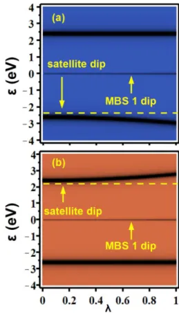
FIG. 5. Parameters employed:M¼0 [long enough Kitaev chain],D¼0.2 [see Eqs.(2)and(53)]. Density plots of the transmittanceTfull(e) determined by Eq.(61)in the Fano regimeqb¼0 [Eq.(64)] as a function of the single particle energyeand the couplingkin units ofD. Implementation of the two-stage procedure of Sec.I: (a)De ¼ þ5 (b)De¼ 5. Here we see the main result of this procedure: the formation of a Majorana dip (in black) pinned at zero-bias even by performing the gates swap. The satellite dips (also in black) do not share such a feature being significantly shifted under the permutation of the levels in the adatoms.
work that the usual hypothesis of the STM tip acting as a probe is insensitive for the complete knowing of the zero-bias transmittance versus the symmetric detuning De. To overcome such an obstacle, the proper description should consider the STM tip in the same footing as the “hostþadatoms” system. It is worth mentioning that we do not present the results for the case qb 1, since it still
obeys the standard Fano’s theory, which gives a resonance profile in theTfull(0) versusDeplot as expected. In Fig. 5
the density plots for Tfull (e) of Eq. (61) with qb¼0 as a
function ofeand the couplingkare shown. In these graphs, dips appear (black color regions) being possible to observe that the MBS 1 dip at zero-bias is the only structure that does not change with the implementation of the two-stage procedure as well as with the increase of k. On the other hand, the positions of the satellite dips are displaced by changingkand no pinning is observed. This feature can be visualized in the dips that deviate from the yellow-dashed lines in Figs. 5(a) and 5(b), respectively, for De¼ þ5 and De¼ 5.
IV. CONCLUSIONS
We have explored theoretically in the context of quan-tum transport an effective Hamiltonian supporting Majorana quasiparticles for a long enough Kitaev chain in the topologi-cal phase. This system is coupled to a setup made by an STM tip and a metallic host with two adatoms. Our analysis has revealed that the Green’s functions of the adatoms become symmetric by neglecting the hopping term between one adatom and a side-coupled MBS. However, if we con-sider this parameter relevant, a lack of symmetry manifests in these functions.
To read out this feature experimentally, it has been pro-posed a two-stage procedure of gates swap by using AFM tips. As a result, a persistent zero-bias dip with an ampli-tude nearby 1/2 emerges in the transmittance arising from the isolated MBS under the aforementioned procedure. We have also verified that the fluctuation of the Majorana hall-mark occurs only for the STM tip treated in the same foot-ing as the “hostþadatoms” system. In the case of an STM tip as a probe, the robustness of the Majorana hallmark is kept. However, this small difference between these two Majorana dips results in contrasting Fano profiles for the zero-bias transmittance versus the symmetric detuning. In the case of the STM tip acting as probe, Fano’s theory is confirmed, but with the tip in the same footing as the “hostþadatoms” system, an unexpected Fano lineshape appears. We conclude that to access this non trivial Fano profile, the assumption of an STM tip acting as a probe should not be used.
ACKNOWLEDGMENTS
The authors thank Drs. E. Vernek and J. C. Egues for valuable discussions. This work was supported by the Brazilian agencies CNPq, CAPES and PROPe/UNESP.
1J. Alicea,Rep. Prog. Phys.75, 076501 (2012).
2M. Leijnse and K. Flensberg,Phys. Rev. B84, 140501(R) (2011). 3
H.-F. L€u, H.-Z. Lu, and S.-Q. Shen,Phys. Rev. B86, 075318 (2012). 4
M. Leijnse and K. Flensberg,Phys. Rev. B86, 134528 (2012). 5K. Flensberg,Phys. Rev. Lett.106, 090503 (2011).
6M. Leijnse and K. Flensberg,Phys. Rev. Lett.107, 210502 (2011). 7
A. Y. Kitaev,Phys. Usp.44, 131 (2001). 8
Y. Cao, P. Wang, G. Xiong, M. Gong, and X.-Q. Li, Phys. Rev. B86, 115311 (2012).
9M. Gibertini, F. Taddei, M. Polini, and R. Fazio,Phys. Rev. B85, 144525
(2012). 10
L.-J. Lang and S. Chen,Phys. Rev. B86, 205135 (2012).
11C.-H. Lin, J. D. Sau, and S. Das Sarma,Phys. Rev. B86, 224511 (2012). 12X.-J. Liu and A. M. Lobos,Phys. Rev. B87, 060504(R) (2013). 13
D. Sticlet, C. Bena, and P. Simon,Phys. Rev. B87, 104509 (2013). 14
J. Liu, A. C. Potter, K. T. Law, and P. A. Lee,Phys. Rev. Lett. 109, 267002 (2012).
15S. Nakosai, J. C. Budich, Y. Tanaka, B. Trauzettel, and N. Nagaosa,Phys.
Rev. Lett.110, 117002 (2013). 16
D. Roy, C. J. Bolech, and N. Shah,Phys. Rev. B86, 094503 (2012). 17G. Moore and N. Read,Nucl. Phys.360, 362 (1991).
18L. Fu, C. L. Kane, and E. J. Mele,Phys. Rev. Lett.98, 106803 (2007). 19
L. Fu and C. L. Kane,Phys. Rev. Lett.100, 096407 (2008). 20
J. D. Sau, R. M. Lutchyn, S. Tewari, and S. Das Sarma,Phys. Rev. Lett.
104, 040502 (2010).
21C. J. Bolech and E. Demler,Phys. Rev. Lett.98, 237002 (2007). 22
D. E. Liu and H. U. Baranger,Phys. Rev. B84, 201308(R) (2011). 23
E. Vernek, P. H. Penteado, A. C. Seridonio, and J. C. Egues, e-printarXiv: 1308.0092v2 [cond-mat.mes-hall](2013).
24V. Mourik, K. Zuo, S. M. Frolov, S. R. Plissard, E. P. A. M. Bakkers, and
L. P. Kouwenhoven,Science336, 1003 (2012). 25
A. Das, Y. Ronen, Y. Most, Y. Oreg, M. Heiblum, and H. Shtrikman, Nature Phys.8, 887 (2012).
26A. C. Hewson, The Kondo Problem to Heavy Fermions (Cambridge
University Press, Cambridge, England 1993). 27
D. Goldhaber-Gordon, H. Shtrikman, D. Mahalu, D. Abusch- Magder, U. Meirav, and M. A. Kastner,Nature391, 156 (1998).
28S. M. Cronenwett, T. H. Oosterkamp, and L. P. Kouwenhoven,Science
281, 540 (1998). 29
A. F. Otte, M. Ternes, K. V. Bergmann, S. Loth, H. Brune, C. P. Lutz, C. F. Hirjibehedin, and A. J. Heinrich,Nature Phys.4, 847 (2008).
30V. Madhavan, W. Chen, T. Jamneala, and F. Crommie,Phys. Rev. B64,
165412 (2001). 31
N. Knorr, M. A. Schneider, L. Diekh€oner, P. Wahl, and K. Kern,Phys. Rev. Lett.88, 096804 (2002).
32C. Y. Lin, A. H. C. Neto, and B. A. Jones,Phys. Rev. Lett.97, 156102
(2006). 33
M. Ternes, A. J. Heinrich, and W. D. Schneider,J. Phys.: Condens. Matter
21, 053001 (2009).
34U. Fano,Phys. Rev.124, 1866 (1961). 35
A. E. Miroshnichenko, S. Flach, and Y. S. Kivshar,Rev. Mod. Phys.82, 2257 (2010).
36A. C. Seridonio, E. C. Siqueira, F. M. Souza, R. S. Machado, S. S. Lyra,
and I. A. Shelykh,Phys. Rev. B88, 195122 (2013). 37