Transient Stability Analysis of a Three-machine Nine Bus Power System Network

Transient Stability Analysis of a Three-machine

Nine Bus Power System Network

M. A. Salam, M. A. Rashid, MemberIAENG, Q. M. Rahman and M. Rizon

Abstract-Transient stability analysis plays an important role for planning, designing and upgrading an existing electrical power system network. In this paper, transient stability analysis is carried out by considering a three-phase fault at the busbars 7 and 4 with the effect of various fault-clearing times. The simulation is carried out using CYME 5.02 power system software with fast decoupled method. It is found that at fault clearing times of 0.05s, 0.1s, and 0.15s, the generators (G2, G3) under test are stable with respect to the simulation time. Whereas, at fault clearing times of 0.2s and 0.3s, these generators are found to be unstable for both faulted busbars 7 and 4. These simulation results are then compared with the proposed model results and are found to be in good agreement. In addition, it has been demonstrated that the transient stability of a system can be improved using control devices.

Keywords: Transient stability, CYME software, three-machine, three-phase fault, fault clearing times, stable, unstable, control devices.

I. INTRODUCTION

AY by day demand of electrical power is increasing due to expansion of industrial, residential and commercial sectors. In this regard, electric utility companies are being asked to run their machines very close to their maximum output. To meet this demand, the size of the interconnected power system is increasing, which in turn is resulting in an increase in the modification cost of these power systems. The utility companies are planning and adopting wide range of design options to reduce the higher modification cost. In this circumstance, detail studies related to transient stability analysis are carried out by considering different assumptions. Transient stability analysis requires huge amount of computational efforts due to large size of interconnected power system. Due to network complexity, power system stability is divided into smaller areas including rotor angles, frequency and voltage stabilities. Rotor angle stability refers to the ability of synchronous machines of an interconnected power systems to remain in synchronism after being subjected to a fault [1-2]. N. Amjady and S. F. Majedi [2] have proposed a new hybrid intelligent system for prediction of transient stability. Manuscript received August 30, 2013; revised February 2, 2014.

M. A. Salam is with the Dept. of Electrical and Electronic Engineering, Institute Technology Brunei, Brunei Darussalam.

M. A. Rashid is with the Faculty of Design Arts and Engineering Technology, Universiti Sultan Zainal Abidin (UniSZA), Kuala Terengganu, Malaysia (phone: +60-164243-521, e-mail: rashid68@yahoo.com). Q. M. Rahman is with the Dept. of Electrical and Computer Engineering, University of Western Ontario, London, ON, N6A 5B9, Canada.

M. Rizon is with the Faculty of Design Arts and Engineering Technology, UniSZA, Kuala Terengganu, Malaysia.

In their paper, the intelligent system is composed of a processor, an array of neural networks (NN) and an interpreter.

In [3], the authors have demonstrated that the study of transient stability of a system is important not only for design and coordination of protection scheme at the planning stage but also for security control during system operation. A. M. Mihirig and M. D. Wvong [4] have proposed a catastrophe theory to determine the transient stability regions of multimachine power systems. They have calculated transient stability limits from the bifurcation set and the critical clearing time from the catastrophe manifold equation. Distributed approach for real time transient analysis have already been mentioned by some authors (e.g., see [5]) describing stability analysis for large number of machines and busbars. A direct method of Lyapunov functions has been used to recognize the fault location as a critical factor for the determining the boundary of the stability region [6].

A new method has been developed for economic dispatch together with nodal price calculations which included transient stability constraints and, at the same time, optimized the reference inputs to the flexible AC transmission system (FACTS) devices for enhancing system stability and reducing nodal prices [7, 8].

The accuracy of using static (nonlinear) load models with suitably identified parameters for transient stability analysis has been examined in [9]. Here, numerical studies have been conducted using on-line measurement data for modeling real power behaviors during disturbances and hence were deemed adequate for transient stability analysis. In [10], the authors have carried out Transient stability analysis in different cases such as peak and off-peak loads, connection and disconnection of busbar, with and without current limit reactor (CLR). In this case, the transient stability in peak load condition was more stable than that in off-peak load condition; the transient stability with bus-bar disconnected was more stable than that with bus-bar connected; the transient stability with CLR was more stable than that without CLR. Transient stability analysis in terms of machines rotor angle, electrical power, machines speed and terminal voltage has been done for Sarawak grid system using power system simulation for engineers in [11]. A power system analysis toolbox (PSAT) was used to study transient stability analysis for the IEEE 14-bus system with wind connected generator in [12]. Systematic investigations of transient stability analysis have been conducted by the combination of step-by-step integration and direct methods in [13]. In this case, more time was required to calculate potential and kinetic energies of all machines before and after the faults. Carlo Cecati and Hamed Latafat [14] have

studied transient stability of a two-machine infinite bus by time-domain versus transient energy function when affected by large disturbances. Here, they have used the Lyapunov function and decentralized nonlinear controller to study transient stability.

In this paper, a new method, based on control theory, has been proposed to overcome the drawbacks of different existing methods. In addition, CYME 5.02 simulation software is used to simulate the transient stability analysis by considering three-phase fault at busbars 4 and 7. The simulation results have been compared with the results obtained by the proposed method.

II.PROPOSED METHOD

The proposed method is developed based on the swing equation and the theory of control system. The well-known classical swing equation which is related to synchronous generator rotor swing angle is [15],

2

2 a m e

d

M P P P

d t 

   (1) Where, 2 s H M 

 , (2)

a

P is the accelerating power,

m

P is the mechanical power,

e

P is the electrical power output,

s

 is the synchronous angular velocity of the rotor,



is the synchronous machine rotor angle,

H is the inertia constant.

The power output of the single machine connected to an infinite bus at any instant of time is,

sin

e mxm

P P  (3)

The mechanical power input equal to the prefault electrical power output at an initial angle ₀is given as,

0

sin

m mxm

P P  (4)

At any location of the network, the system reactance during the occurrence of a fault is different from the reactance after clearing the fault. As a result, the corresponding output powers in these two conditions are found to be different. In this case, the maximum value of the machine output power Pmxm can be represented as a

two-valued step function as shown in Fig.1 and this can be represented as [16],

1 ( ) ( )

mxm r

P Pu t  u tt (5) Where,

( )

u t is the step function at t0, ( _r)

u tt is the step function at tt_r,

2 1

P P

   ,

1

P is the maximum power output during the occurrence of a fault, and

2

P is the maximum power output after removing the fault. The rotor swing angle



, which has been defined relative to a reference axis rotating at the synchronous angular velocity

s

 , can be expressed in terms of the actual rotor speed  as,

( _s)t 't

     (6) Differentiating equation (6) with respect to tprovides,

' d 2 f'

dt 

    (7)

Where,



'is a measure of the frequency ( ')f of rotor oscillation with respect to the synchronously rotating reference axis.

Considering the following relation: sin

y  (8)

Substituting equation (6) into equation (8), yields, sin '

y  t (9)

Substituting equations (5) and (9) into equation (3) provides,

1sin ' ( ) sin ' ( )

e r

P P  t u t    t u tt (10)

Taking Laplace transform of equations (1), (7), (9)

2

( ) _a( ) _m( ) _e( )

Ms  s P s P s P s (11)

2 ' ( )s

s 

  (12)

2 2 ' ( ) ' Y s S   

 (13)

1

2 2 2 2

' ( 'cos ' sin ' )

( ) ' ' r t s r r e

P e t s t

P s s s           

  (14)

Equation (11) provides the transfer function of the forward path block of Fig. 2 and it can be expressed as,

2

( ) 1

( ) ( )

a s G s

P s Ms



  (15)

Dividing equation (13) by equation (12), yields the transfer function of the first feedback block,

2

1 _{2 2}

( ) ( )

( ) '

Y s s

H s

s s

 

 

 (16)

Dividing equation (14) by equation (13) gives the transfer function of the second feedback block as,

2 1

( ) ( 'cos ' sin ' )

( )

( ) '

r t s

e r r

P s e t s t

H s P

Y s

  





 

   (17)

In taking Laplace transforms the rotor oscillation angular velocity



'has been considered to be constant at an average value. The closed loop transfer function of the feedback system of Fig.2 corresponding to a synchronous machine is,

1 2

( ) ( )

( ) 1 ( ) ( ) ( )

m

s G s

P s G s H s H s

 _

 (18) Substituting the expressions of G(s), H1(s), and H2(s) into

equation (18) gives,

2

2

1

2 2 2

1 ( )

( ) _{1 ( 'cos ' sin ' )}

1

' '

r t s

m _{r r}

s _Ms

P s _{e t s t s}

P Ms s                 _  _{ } _  _{  } (19)









2 2 2 2

1 2 3

1 ' ( )

( ) t sr t sr

m

s

s _M

P s s s k k e k se  

 

 

   (20)

1 P 2 P mxm P r t 0 t  2 1 1 ' P k M 

  (21)

2 1

' cos '_r

k t

M  

  (22)

3 sin ' ' r t k M   

 (23) The characteristic equation of the feedback system of Fig. 2

derived from the swing equation of a synchronous machine is the denominator of equation (20) equated to zero as shown below:

2

1 2 r 3 r 0

t s t s

s  k k e k se  (24) Equation (24) can be rewritten as follows:

1 2

( ) ( ) ( ) 0

f s  f s  f s  (25) Where,

2

1( ) 1

f s s k (26)

3

2 2

2

( ) t sr 1 k

f s k e s

k

  

 _  _

  (27)

It is evident that a root of equation (25) is the point of intersection of the functions f s₁( )and f s₂( ). This point has been termed as the dominant root. Fig.3 shows the sketches of the forms of the functions f s₁( )andf s₂( ). It can be seen that function f s₁( ) is greater than f₂( )s i.e.

1 2

( ) ( ) ( )

f s  f s  f s is positive for all values of s on the right of and up to the point 2

3

k s

k

  . At 2

3

k s

k

  , the

function f₂( )s is zero and beyond this point f₂( )s starts increasing so that f₂( )s intersects f s₁( )at a point having its real part equal to s_root. This point is the desired dominant root to be searched for. Beyond this point s_root, f₂( )s is greater than

1( )

f s i.e. the function ( )f s is negative.

Fig. 1 Maximum power output during and after faults.

Fig. 2 Represented swing equation into a feedback model.

Therefore, a search for the real axis bounds of the region containing the dominant root can be made starting from the

point 2

3

k s

k

  and continued by increasing the absolute

value of s until the function ( )f s becomes negative.

Fig. 3 Sketches of functions f s₁( )and f s₂( ). III.RESULTS AND DISCUSSION

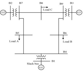
The CYME software is used to study the transient stability analysis of the IEEE three-machine, nine-busbar power system network. The base MVA and system frequency are considered to be 100 MVA and 60 Hz, respectively. The single-line diagram of the three-machine power system is shown in Fig. 4. Here, generator G1 is connected to slack bus 1, whereas generators 2 (G2) and 3 (G3) are connected to busbars 2 and 3, respectively. Loads A, B and C are connected in busbars 5, 6 and 8 respectively. Initially, fast decoupled method is used for load flow analysis. Then transient stability analysis has been carried out by monitoring the performance of the generators (G1, G2 and G2) and different buses. Two cases have been considered in the transient stability analysis of this power system network. The simulation results based on the fast decoupled method and the proposed method were compared.

Fig. 4 Single-line diagram of three machine power system.

This comparison rendered the required minimum average distance of the dominant roots on the left of the imaginary axis. The power system network can be identified as either stable or unstable based on the minimum average distance of the dominant roots as shown by the proposed method.

2 1 ( ) G s Ms  ( ) a P s 2 1

( ' cos ' sin ' )

( )

'

r

t s

r r

e t s t

H s P   





 

 

2 1( ) 2 2

' s H s s    ( ) e P s ( ) m P s ( ) Y s  

( )s  1 k ( ) f s 2 k 0 s 2 k  1 

1( )

f s 2

1( ) 1

f s s k

root s 2 3 k s k  

2( )

f s

3

2 2

2

( ) t sr ( 1 k )

f s k e s

k 

  

2 r

t s

0 0.2 0.4 0.6 0.8 1 1.2

0 0.5 1 1.5 2 2.5 3

B

4

The first case has been dealt with a three-phase fault occurring near bus 7 of the line 5-7 and, considered a number of fault clearing times (fct) of 0.05s, 0.1s, 0.15s, 0.2s and 0.3s, respectively.

Fig.5. SM relative rotor angles when fault at bus 7 and fct 0.05s.

Fig 6.SM relative rotor angles when fault at bus 7 and fct 0.1s.

Fig.7.SM relative rotor angles when fault at bus 7 and fct 0.15s.

Fig.8.SM relative rotor angles when fault at bus 7 and fct 0.2s.

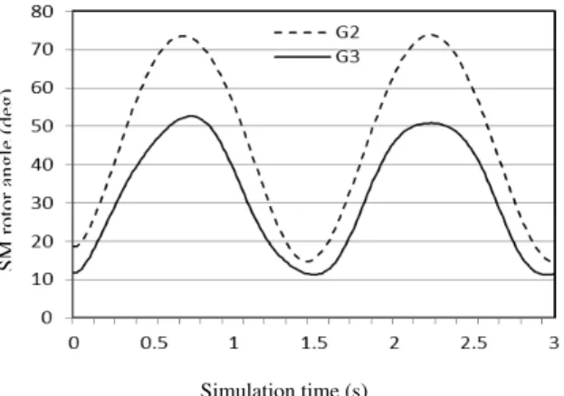
The fault is cleared by disconnecting the line 5-7 and, the duration of simulation is considered to be 180 cycles (3s). The swing angles of the generators G2 and G3 have been calculated by subtracting the swing angles of the generator G1 for different fault clearing times. Then the swing angles of generators G2 and G3 are plotted in the



t plane, which are shown in Figs. 5 to 8.An inspection of Figs. 5, 6, and 7 shows that the three-machine system is stable for the first three fault clearing times of 0.05s, 0.1s, and 0.15s, because relative rotor angles of G2 and G3 swing together with respect to the simulation time.

Fig. 9.SM relative rotor angles when fault at bus 7 and fct 0.3s.

From Figs. 8 and 9, it is found that relative rotor angles of the generators G2 and G3 increases abnormally to 2800 degree instead of swinging with the simulation time.

Fig.10. Busbar voltage fault at bus 7 and fct 0.1s.

Fig.11. Busbar voltage fault at bus 7 and fct 0.15s. Simulation time (s)

Simulation time (s)

Simulation time (s)

Simulation time (s) Simulation time (s)

Simulation time (s)

Simulation time (s)

SM

ro

tor

angle

(deg)

SM

ro

tor

angle

(deg)

SM

ro

tor

angle

(deg)

SM

ro

tor

angle

(deg)

Busbar

voltage (

pu)

SM

ro

tor

angle

(deg)

Busbar

voltage (

0 0.2 0.4 0.6 0.8 1 1.2

0 0.5 1 1.5 2 2.5 3

B4

B7

B9

0 0.2 0.4 0.6 0.8 1 1.2

0 0.5 1 1.5 2 2.5 3

B4

B7

B9

This characteristic indicates that both generators are unstable for the fault clearing times of 0.2s and 0.3s respectively. The voltages at the buses 4, 7 and 9 for the fault clearing times of 0.1s, 0.15s, 0.2s and 0.3s are shown in Figs. 10, 11, 12 and 13, respectively.

Fig.12. Busbar voltage fault at bus 7 and fct 0.2s.

Fig.13. Busbar voltage fault at bus 7 and fct 0.3s.

From Figs. 10 and 11, it is observed that the busbar voltage is collapsed at the fault clearing times of 0.1s and 0.15s respectively. After that, the busbar voltages swing together with the simulation time, which indicates that the generators G2 and G3 are becoming stable. The bus voltages have been collapsed at the fault clearing times of 0.2s and 0.3s as can be seen in Figs. 12 and 13. After the fault, these voltages did not swing together with the simulation time, which caused unstable condition.

The results obtained by the application of the proposed method in case I with a choice of 0.25 Hz for the rotor oscillation frequency of all machines have been shown in Table 1. From Table 1, it should be noted that the average distances of the dominant roots of the three machines from the imaginary axis for the first three faults clearing times of 0.05s, 0.1s, and 0.15s are -72.95, -21.91 and -10.87, respectively. For stable condition, the minimum average distance of the dominant roots is considered to be -10.87. In this light, the power system network represents stable condition for the fault clearing times of 0.05s, 0.1s and 0.15s. For the last two fault clearing times (0.2s, 0.3s), the average distance is very less than the minimum average distance of the dominant roots that makes the system

unstable. A comparison with the swing curves in Figs. 5 to 9 obtained by the simulation for the same fault clearing times also validates the results on stability by the proposed method as shown in Table 1.

In the second case, a three-phase fault is considered near bus 4 of the line 4-6. Then the load flow solution is carried out and the transient stability is performed for the fault clearing times (fct) of 0.05s, 0.1s and 0.3s respectively by opening the line 4-6. The swing angles of the generators G2 and G3 are determined by subtracting the swing angles of the generator G1 at an interval of 0.01s for a simulation time of 3s by the CYME 5.02 software and plotted in Figs. 14 to 16.

Fig.14. SM relative rotor angles when fault at bus 4 and fct 0.05s.

Fig.15. SM relative rotor angles when fault at bus 4 and fct 0.1s.

Fig.16. SM relative rotor angles when fault at bus 4 and fct 0.3s. Simulation time (s)

Simulation time (s)

Simulation time (s)

Simulation time (s)

Simulation time (s)

SM

ro

tor

angle

(deg)

Busbar

voltage (

pu)

Busbar

voltage (

pu)

SM

ro

tor

angle

(deg)

SM

ro

tor

angle

From Figs. 14 to 16, it is observed that the system is stable for the fault clearing times of 0.05s and 0.1s respectively. It is unstable for the fault clearing time of 0.3s as the second swing is decreasing than the first swing of the generator G3. The results obtained by the proposed method for case II with a rotor oscillation frequency of 0.25 Hz is shown in Table 2. In case I, it is found that the minimum average distances of the roots on the left of the imaginary axis in s-plane must be -10.87 to consider the three-machine system stable. Therefore, it should be noted in Table 2 that the system is stable for case II for the fault clearing times of 0.05s and 0.10s when the average distance of the dominant roots on the left of the imaginary axis is more than -10.87. Since for the fault clearing time of 0.3s, the average distance is only -3.08 on the left of the imaginary axis, the system is indicated to be unstable.

Fig.17. SM relative rotor angles when fault at bus 7 and fct 0.2s.

Fig.18. SM relative rotor angles when fault at bus 7 and fct 0.3s.

The simulation is then repeated to analyze the transient stability of the power system network by considering the effect of the exciter and the governor. In this case, the IEEE model of salient pole synchronous generator with automatic voltage regulator as the excitation system and diesel governor is used to improve the stability. The same fault clearing times (0.2s and 0.3s) are repeated for this simulation and the relative rotor angles for the generators are then plotted as shown in Figs. 17 and 18 respectively. The relative rotor angles of generators G2 and G3 swing smoothly up to 1s, whereas the angles increases together after 1s and again swing with simulation time. When

compared to the results plotted in Figs. 8 and 9 with the corresponding results plotted in Figs. 17 and 18, it is seen that both generators G2 and G3 are in stable condition. Therefore, it can be concluded that the transient stability can be improved using control devices such as exciter and governor.

TABLE I

STABILITY RESULTS FOR A FAULT NEAR BUS 7 ON LINE 5-7 IDENTIFYING DOMINANT ROOTS CORRESPONDING TO A

ROTOR OSCILLATION FREQUENCY OF 0.25 HZ Fault

clearing time

(s)

Starting point for root search

Average number of search steps in increment

of -10

Average of the lower limits of roots locations in s-plane

Remarks

0.05 -19.95 7 -72.95 Stable

0.1 -9.91 3 -21.91 Stable

0.15 -6.54 2 -10.87 Stable

0.2 -4.83 2 -6.83 Unstable

0.3 -3.08 2 -3.41 Unstable

TABLE II

STABILITY RESULTS FOR A FAULT NEAR BUS 4 ON LINE 4-6 IDENTIFYING DOMINANT ROOTS CORRESPONDING TO A

ROTOR OSCILLATION FREQUENCY OF 0.25 HZ Fault

clearing time

(s)

Starting point for root

search

Average number of search

steps in increment

of -10

Average of the lower

limits of roots locations in

s-plane

Remarks

0.05 -19.95 7 -73.62 Stable

0.1 -9.91 3 -21.58 Stable

0.3 -3.08 2 -3.08 Unstable

IV. CONCLUSION

A new method has been proposed for analyzing transient stability of a three-machine nine bus power system network. This method uses a set of closed loop transfer functions, one for each synchronous generator and is derived by taking Laplace transformation of the nonlinear swing equation. The dominant root is searched in the s-plane for each generator starting from a real value, which is same for all generators and a function of only the rotor oscillation frequency and the fault clearing time. The minimum average distance in the s -plane was deemed to be -10.87 for the three-machine system. A decrement of 10 was found to be quite satisfactory for searching the dominant root. In the stable cases of the system, the average distance of the dominant roots was at or further left of the minimum average distance depending upon the fault clearing time. The average location shifted more towards right with higher fault clearing time and this location was completely on the right of the minimum allowable value for the unstable cases. The simulation was carried out using CYME 5.02 power system software by considering two cases. The simulation results were compared with the proposed method and were found to 0

20 40 60 80 100 120 140

0 0.5 1 1.5 2

SM Ro

to

r An

g

le (d

eg

.)

Simulation time (s) G2

G3

0 50 100 150 200 250

0 0.5 1 1.5 2

SM Rotor angle (deg.)

be in good agreement. Exciter and governor were also used to improve the transient stability of three machines nine busbar system.

REFERENCES

[1] P. Kundur, J. Paserba, V. Ajjarapu, A. Bose, C. Canizares, N. Hatziargyriou, D. Hill, A. Tankovic, C. Taylor, T. Van Catsem, and V. Vittal, “Definition and Classification of Power System Stability-IEEE/CIGRE joint task force on stability terms and definition”, IEEE Transactions on Power Systems, PWS Vol. 19, No. 3, 2004, pp. 1387-1401.

[2] N. Amjadi, S. F. Majedi, “Transient Stability Prediction by a Hybrid Intelligent System”, IEEE Transactions on Power System, PWS Vol. 22, No. 3, 2007, pp. 1275-1283.

[3] M. L. Scala, G. Lorusso, R. Sbrizzai and M. Trovato, “A Qualitative Approach to the Transient Stability Analysis”, IEEE Transaction on Power Systems, PWS Vol. 11, No. 4, 1996, pp. 1996-2002.

[4] A. M. Mihirig and M. D. Wvong, “Transient Stability Analysis of Multimachine Power Systems by Catastrophe Theory”, IEE Proceedings C: Generation, Transmission and Distribution, Vol. 136, No. 4, 1989, pp. 254-258.

[5] G. Aloisio, M. A. Bochicchio, M. La Scala, R. Sbrizzai, “A Distributed Computing Approach for Real Time Transient Stability Analysis”, IEEE Transactions on Power Systems, Vol. 12, No. 2, 1997, pp. 981-987.

[6] A. M. Eskicioglu, O. Sevaioglu, “Feasibility of Lyapunov Functions for Power System Transient Stability Analysis by the Controlling UEP Method”, IEE Proceedings C: Generation, Transmission and Distribution, Vol. 139, No. 2, 1992, pp. 152-156.

[7] T. T. Nguyen, A. Karimishad, “Transient Stability-constrained Optimal Power Flow for Online Dispatch and Nodal Price Evaluation in Power Systems with Flexible AC Transmission System Devices”, IET Generation, Transmission and Distribution, Vol. 5, No. 3, 2011, pp. 332-346.

[8] K. Y. Chan, G. T. Y. Pong and K. W. Chan, “Investigation of Hybrid Particle Swarm Optimization Methods for Solving Transient-Stability Constrained Optimal Power Flow Problems”, Engineering Letters, 16:1, EL_16_1_10, 2008.

[9] H. D. Chiang, B. K. Choi, Y. T. Chen, D. H. Huang, M. G. Lauby, “Representative Static Load Models for Transient Stability Analysis: Development and Examination”, IET Generation, Transmission and Distribution, Vol. 1, No. 3, 2007, pp. 422-431.

[10] O. Zhu, B. Kim, K. Kim, “Transient Stability Analysis on the Offsite Power System of Korean Nuclear Power Plants”, The 46th

Universities Power Engineering Conference, 2011, pp. 1-4, 5-8. [11] A. M. Mohamad, N. Hashim, N. Hamzah, N. F. N. Ismail, M. F. A.

Latip, “Transient Stability Analysis on Sarawak’s Grid using Power System Simulator for Engineers”, IEEE Symposium on Industrial Electronics and Applications, 2011, pp. 521-526, 25-28.

[12] A. G. Pillai, P. C. Thomas, K. Sreerenjini, S, Baby, T. Joseph, S. Srecdharan “Transient Stability Analysis of Wind Integrated Power Systems with Storage using Central Area Controller”, IEEE International Conference on Microelectronics, Communications and Renewable Energy, 2013, pp. 1-5.

[13] H. H. Al-Marhoon, I. Leevongwat, P. Rastgoufard, “A Practical Method for Power System Transient Stability and Security Analysis” IEEE PES Transmission and Distribution Conference and Exposition, 2012, pp. 1-6.

[14] Carlo Cecati and Hamed Latafat, “Time Domain Approach Compared with Direct Method of Lyapunov for Transient Stability Analysis of Controlled Power System”, IEEE International Symposium on Power Electronics, Electrical Drives, Automation and Motion, 2012, pp. 695-699.

[15] M. A. Salam, “Fundamentals of Power Systems”, Alpha Science International Ltd, Oxford, 2009, pp. 336-358.