On the optimum antenna pattern for widebeam radar reflectivity
estimation
F. Gerbl and E. M. Biebl
Fachgebiet H¨ochstfrequenztechnik, Technische Universit¨at M¨unchen, Munich, Germany
Abstract. Noise is a limiting factor in radar systems. The power received from a target depends on the target reflectiv-ity varying with the aspect angle, the target range and the antenna pattern, amongst others. Inevitably, an estimation algorithm for the mean target reflectivity weights noise con-tributions from greater aspect angles stronger than such from smaller aspect angles due to the target range increasing with increasing aspect angle. However, as an opposed effect, due to the supposed equidistant rather than equiangular sampling along the linear aperture, noise contributions for greater as-pect angles have lower influence than those for smaller asas-pect angles. In the paper, the signal-to-noise ratio for a linear, equidistantly sampled aperture and an arbitrary antenna pat-tern is determined. Moreover, an upper limit for the achiev-able signal-to-noise ratio is given, and the antenna pattern maximizing the signal-to-noise ratio is derived.
1 Introduction
Noise is a limiting factor in radar systems. The power re-ceived from a target depends on the target reflectivity vary-ing with the aspect angle, the target range and the antenna pattern, amongst others. Directing power only into a nar-row region of space, i.e. using a high gain antenna, yields higher received power and higher azimuth resolution than transmitting power to a broader region of space. However, using a narrow antenna beam to linearly scan a target scene limits the aspect angles, from which targets with generally unknown orientation are illuminated. Widening the antenna beam and processing the received signal in an appropriate manner, an image containing estimates of the mean target re-flectivities over the aspect angle can be obtained. For wide antenna beams, the range of a target as measured from the Correspondence to: F. Gerbl
radar system, and therefore the power received from even an omnidirectionally scattering target, varies as the radar system passes by the target.
2 Setup
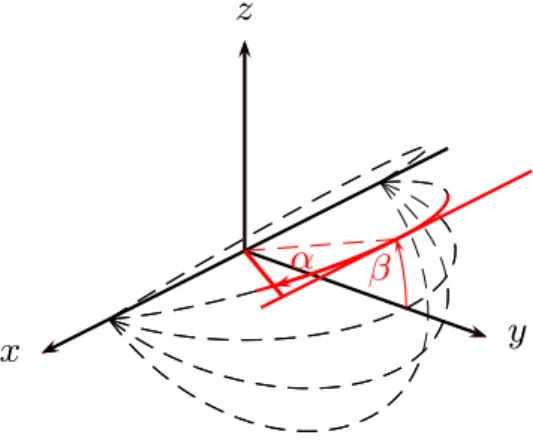
The radar system is moved along a straight path, passing the scene consisting of targets to be imaged. The orientation of the antenna remains unchanged throughout the passing. The system transmits a signal which is reflected by the objects in the scene and in turn received by the system. The amplitude and phase of the received signal are determined and sampled equidistantly along the straight path. The radar system is as-sumed to be monostatic. Figure 1 illustrates the setup and in-dicates the changes the signal undergoes during the passing. Distance and aspect angle and therefore level of free space attenuation, phase shift and the influence of the antenna pat-tern vary as the antenna passes by the target.
3 Coordinate system
an-Fig. 1. Sketch of the setup.
gle coordinate,β, remains constant at the value βt=arctan
zt yt
, (1)
whereytandztare they andzcoordinates of the target. In
Fig. 2, a possible trajectory of a target is indicated with a red line parallel to thexaxis.
4 Signal processing
The received signal is a function of the aspect angleα and timetand can be written as
sRX(α, t )=a·ρ(α)·r21(α)·D 2
A(α)·exp{−j2kr(α)} +nℜ(t )+jnℑ(t )
(2) in the presence of noise, assuming there is only one single point-like target. a is a constant determined by system pa-rameters like radiated power, mixer losses, and others. ρ is the reflectivity of the target, r the distance between an-tenna and target, DA the antenna amplitude pattern, k the
wave number, andnℜ(t )andnℑ(t )are the noise
contribu-tions in real and imaginary part of the received signal, re-spectively. Actually, the antenna pattern is a function of both αandβ. However, since the antenna pattern is assumed to be constant overβ except for a rectangular window that will be accounted for by a proper choice of integration limits, the pattern will be denoted as a function of onlyαinstead ofα andβin the majority of cases in order to avoid unnecessarily long expressions.
Compensating the aforementioned effects and integrating (in reality summarizing) the compensated signals yields a noisy estimateρˆα
0 of the mean reflectivity over the angleα
within±α0
a·2α0· ˆρα0 =
α0 Z
−α0
a·ρ(α)dα+
α0 Z
−α0
n′(α, t )dα (3)
with
n′(α, t )=(nℜ(t )+jnℑ(t ))·r2(α)·
1
DA2(α)·exp{j2kr(α)}, (4)
x
y
z
β
α
Fig. 2. Antenna-centered coordinate systems and trajectory of a
target.
where the estimate consists of the desired signal and a noise contribution. It is desirable to minimize the noise contribu-tion in order to maximize the signal-to-noise ratio.
Throughout the paper, integrals are used for the discussion where possible rather than sums. There remains an uncer-tainty in the estimation of the mean reflectivity due to the non-zero distance between two samples. However, the spac-ing has to be chosen relatively small in order to avoid aliasspac-ing in case of wide antenna beams. It is assumed that the spacing is so small that sum and integral can be regarded as equal.
For that pixel of the reflectivity map that corresponds to the true target location, the signal-to-noise ratio of the processing result is
SNR= S
N, (5)
where
S=
α0 Z
−α0
a·ρ(α)dα 2
=
a·2α0·ρα0 2
(6)
is the power of the desired signal and
N =E
α0 Z
−α0
n′(α, t )dα
2
. (7)
is the mean power of the noise contribution after process-ing. E{·}denotes the expected value. Note thatN is not the power of the noise contributionsnℜ(t )andnℑ(t )but that of
the noise in the processing result. It is shown in Appendix A that the SNR can be written as
SNR= 4α
2 0 a·ρα0
2
1x·r03·Pn′·
α0 R
−α0 1
D2(α)cos2(α)dα
5 Optimization
From Eq. (8) it is obvious that the SNR is influenced by the antenna pattern. The antenna pattern is to be optimized in that sense that the SNR after the signal processing is maxi-mized, i.e. the expression
α0 Z
−α0
1
D2(α)cos2(α)dα (9)
in the denominator of Eq. (8) is to be minimized. The bound-ary condition for the optimization is generally
Z Z
D()d=4π, (10)
and particularly for the coordinate system used here π
Z
−π π/2 Z
−π/2
D(α, β)cos(α)dαdβ=4π. (11)
i.e. the integral of the antenna pattern over all solid angle elements of a sphere has to be equal to 4π.
The first step to maximizing the SNR is to restrict the radi-ation to only those regions of space from where signals will be processed. For a given maximum processing angleα0, the
antenna pattern has to vanish for|α|>α0. For the following
considerations it is assumed that the antenna pattern does not vary with the angleβexcept for the fact that the pattern van-ishes for|β|>β0resulting in a limited field of view, within
which the SNR is independent of the target’s location with respect to the related angle β. Under the prerequisites of a pattern vanishing for|α|>α0and|β|>β0and being
con-stant with respect toβinside its support region, the boundary condition can be written as
2β0
α0 Z
−α0
D(α)cos(α)dα=4π. (12)
It is shown in Appendix B that the optimum antenna pattern, Dopt,α0, for a given maximum processing angleα0that
max-imizes the SNR is Dopt,α0(α)=
π
α0β0 · 1
cos(α) for |α| ≤α0and |β| ≤β0
0 else .(13)
-90
-60 -30
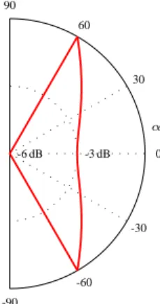
Fig. 3. Normalized optimum patternDopt,α0(α)forα0=60
◦.
For every maximum processing angleα0, a different antenna
pattern is optimum. Using the respective pattern, the maxi-mum achievable signal-to-noise ratio SNRmaxcan be
deter-mined with Eqs. (8) and (13) to be
SNRmax=
2π2aρα 0
2
1x·r03·P′
n·α0·β02
. (14)
The maximum achievable signal-to-noise ratio decreases with increasing antenna beam width. Nevertheless, there might be reasons (e.g. decreasing the probability of missing a target that reflects strongly anisotropically, increasing az-imuth resolution) to use wide antenna beams. The signal-to-noise ratio is only one figure of merit amongst others. Using the appropriate optimum pattern yields the maximum achiev-able SNR for a givenα0. Figure 3 shows exemplarily the
optimum pattern forα0=60◦.
6 Benefit of the findings
Equation (8) allows the determination of the achievable SNR for a given antenna pattern and a certain maximum process-ing angle α0 that might be dictated by special needs of a
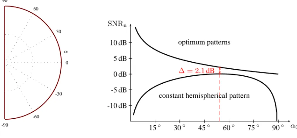
certain application. Equation (14) provides a benchmark for the antenna under consideration. The Figs. 4, 5 and 6 show three different antenna patterns and the resulting normal-ized signal-to-noise ratios for different maximum processing angles α0 along with the normalized maximum achievable
signal-to-noise ratios using the appropriate optimum patterns matched to the respective maximum processing angles. Ref-erence for the normalization is the signal-to-noise ratio ob-tainable forα0=90◦with the respective optimum pattern.
Figure 4 shows the normalized pattern (red) of an an-tenna that radiates power uniformly into all directions of the hemisphere. Nominally, this antenna has a beam width of
-90
-60 -30
0 30 60 90
α
optimum patterns
constant hemispherical pattern
15◦ 30◦ 45◦ 60◦ 75◦ 90◦ α0 -10 dB
-5 dB 0 dB 5 dB 10 dB SNRn
∆ = 2.1dB
Fig. 4. Plot of a constant hemispherical pattern (red) and the resulting normalized signal-to-noise ratios compared to the optimum pattern.
-90
-60 -30
0 30 60 90
α
-12 dB -6 dB
optimum patterns
patch pattern
15◦ 30◦ 45◦ 60◦ 75◦ 90◦ α0
-10 dB -5 dB 0 dB 5 dB 10 dB
SNRn
∆ = 3.1dB
Fig. 5. Plot of the pattern of a patch antenna (red) and the resulting normalized signal-to-noise ratios.
this pattern is about 2.1 dB below that achievable with the re-spective optimum pattern.
Figure 5 shows the normalized pattern (red) of a patch an-tenna. Its optimum maximum processing angle isα0≈31◦. The pattern plot also shows the pattern (black) of the opti-mum pattern forα0=31◦. The maximum signal-to-noise ra-tio achievable with the patch pattern is about 3.1 dB below that achievable with the respective optimum pattern.
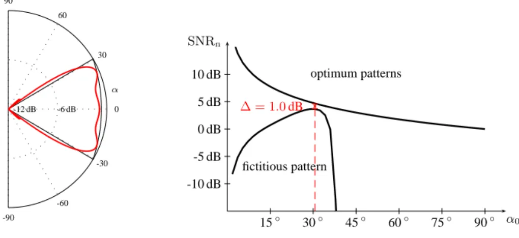
Figure 6 shows a fictitious pattern (red) as it might emerge during the design process of an antenna. Its optimum max-imum processing angle isα0≈31◦as for the patch antenna considered before. The pattern plot also shows the pattern (black) of the optimum pattern forα0=31◦. The maximum
signal-to-noise ratio achievable with this fictitious pattern is about 1 dB below that achievable with the respective opti-mum pattern. The reason for the drop-off of the signal-to-noise ratio for angles above the optimum angle is that only a very small fraction of the energy is radiated into the re-spective directions and the compensation of signals received
from those directions causes strong noise contributions due to a multiplication with the reciprocal of the almost vanishing antenna pattern.
The curve of the maximum achievable signal-to-noise ra-tio given by Eq. (14) can be used advantageously to judge the quality of the approximation of a desired antenna pattern by the current design.
7 Conclusions
-90
-60
-30 fictitious pattern
15◦ 30◦ 45◦ 60◦ 75◦ 90◦ α0 -10 dB
-5 dB 0 dB
Fig. 6. Plot of a fictitious pattern (red) and the resulting normalized signal-to-noise ratios.
can be used to evaluate the performance of existing antennas for the task of estimating the radar reflectivity within differ-ent maximum processing angles. The results show that the signal-to-noise ratio achievable with a certain pattern as it might emerge in one of the iterations of an antenna design process does not depend on single values of the pattern but on an integral over a function of the antenna pattern. Thus, the difference of the signal-to-noise ratio achievable with the pattern under consideration and that achievable with the ap-propriate optimum pattern can be used as a figure of merit for the evaluation of an antenna pattern.
Appendix A Determination of the signal-to-noise ratio
Content of this section is the derivation of Eq. (8). Samples of the received signal are taken equidistantly at discrete po-sitions along a straight line. Therefore, the number of sam-ples per angle element is greater for greater anglesαthan for smaller ones. To account for this fact, the statistical evalua-tion of the noise contribuevalua-tion has to be done after the substi-tution ofαbyx. With
α=arctan x r0
, dα
dx = r0
r02+x2 (A1)
Equation (7) can be written as
N =E
x0 Z
−x0
n′(α(x), t ) r0 r02+x2dx
2
. (A2)
Using
r02+x2≡r2(α(x)) (A3)
and
n′′(α(x), t )=n
′(α(x), t )
r2(α(x)) , (A4)
the noise power after processing reads as
N =r02E
x0 Z
−x0
n′′(α(x), t )dx
2
(A5)
and consequently
N =r02E
x0 R
−x0 ℜ
n′′(α(x), t ) dx !2
+
x0 R
−x0 ℑ
n′′(α(x), t ) dx !2
=r02 EX21 +EX22
(A6)
with
X1=
x0 Z
−x0 ℜ
n′′(α(x), t ) dx (A7)
and
X2=
x0 Z
−x0 ℑ
n′′(α(x), t ) dx. (A8)
The integrands are
ℜ
n′′(α(x), t ) =
nℜ(t )cos(2kr(α(x)))−nℑ(t )sin(2kr(α(x)))
D(α(x)) (A9)
and
ℑ
n′′(α(x), t ) =
nℜ(t )sin(2kr(α(x)))+nℑ(t )cos(2kr(α(x)))
nℜ(t )andnℑ(t )are zero-mean. Therefore, the sum of several
samples of those noise processes is zero-mean:
E{X1} =E{X2} =0. (A11)
Since generally
EnX2o=Var{X} +E2{X} (A12)
and under the prerequisite thatnℜ(t )andnℑ(t )have the same
properties, it can be stated that
EnX12o=EnX22o=Var{X1} =Var{X2}. (A13)
Therefore,
N =2r02Var{X1}. (A14)
For further evaluation, the integrals are temporarily approxi-mately replaced by sums. The reason is that in the continuous integral two “samples” of the noise process are directly ad-jacent to each other and therefore correlated. In reality, sam-ples are taken with non-zero intervals between them. Assum-ing that those intervals are great enough, which is satisfied in many cases in reality, two samples of the noise process can be treated as uncorrelated. With the substitution
f (x)=2kr(α(x)), (A15)
the variance ofX1can be evaluated as
Var{X1}
=Var x0 Z
−x0
nℜ(t )cos(f (x))−nℑ(t )sin(f (x))
D(α(x)) dx ≈Var ( l 0 X
l=−l0
nℜ(t )cos(f (l1x))
D(α(l1x)) 1x
−
l0 X
l=−l0
nℑ(t )sin(f (l1x))
D(α(l1x)) 1x
)
=1x2Var ( l
0 X
l=−l0
nℜ(t )cos(f (l1x))
D(α(l1x)) )
+1x2Var ( l
0 X
l=−l0
−nℑ(t )cos(f (l1x))
D(α(l1x)) )
=1x2 l0 X
l=−l0
Var n
ℜ(t )cos(f (l1x))
D(α(l1x))
+1x2 l0 X
l=−l0
Var
−nℑ(t )cos(f (l1x))
D(α(l1x))
=1x2Var{nℜ(t )}
l0 X
l=−l0
cos(f (l1x)) D(α(l1x))
2
+1x2Var{nℑ(t )}
l0 X
l=−l0
−sin(f (l1x)) D(α(l1x))
2
=1
2 ·1x·P
′
n·
l0 X
l=−l0
1
D2(α(l1x))1x
≈1
2 ·1x·P
′
n·
x0 Z
−x0
1 D2(α(x))dx.
(A16)
With the substitution x=r0tanα, dx=
r0
cos2(α)dα (A17)
and Eqs. (8), (6), (7), (A16), the the maximum achievable signal-to-noise ratio can be written as in Eq. (14).
Appendix B Optimization
Content of this section is the minimization of expression (9) with the boundary condition (12) by means of Lagrange mul-tipliers and the calculus of variations. With the substitution
y(α)=D(α)cos(α), (B1)
the Lagrange functional
F (α)=
α0 Z
−α0
1
y2(α)+λy(α)
dα−λ2π β0
=
α0 Z
−α0
f (y(α))dα−λ2π β0
(B2)
with
f (y(α))= 1
y2(α)+λy(α) (B3)
can be formed. A necessary condition forD being an ex-tremal is
fy=0. (B4)
This condition is fulfilled by
D(α)= 2
λ 13
· 1
lows.
Acknowledgement. The authors would like to thank K. Frick, Insti-tute of Computer Science, University of Innsbruck, Austria, for the fruitful correspondence regarding the optimization method.