Automated Learning of Subcellular Variation
among Punctate Protein Patterns and a
Generative Model of Their Relation to
Microtubules
Gregory R. Johnson1,2, Jieyue Li2,3, Aabid Shariff1,2, Gustavo K. Rohde1,2,3,4‡, Robert F. Murphy1,2,3,5,6‡*
1Computational Biology Department, Carnegie Mellon University, Pittsburgh, Pennsylvania, United States of America,2Center for Bioimage Informatics, Carnegie Mellon University, Pittsburgh, Pennsylvania, United States of America,3Department of Biomedical Engineering, Carnegie Mellon University, Pittsburgh, Pennsylvania, United States of America,4Department of Electrical and Computer Engineering, Carnegie Mellon University, Pittsburgh, Pennsylvania, United States of America,5Departments of Biological Sciences and Machine Learning, Carnegie Mellon University, Pittsburgh, Pennsylvania, United States of America, 6Faculty of Biology and Freiburg Institute for Advanced Studies, Albert Ludwig University of Freiburg, Freiburg, Germany
‡These authors are joint senior authors on this work. *[email protected]
Abstract
Characterizing the spatial distribution of proteins directly from microscopy images is a diffi-cult problem with numerous applications in cell biology (e.g. identifying motor-related pro-teins) and clinical research (e.g. identification of cancer biomarkers). Here we describe the design of a system that provides automated analysis of punctate protein patterns in micro-scope images, including quantification of their relationships to microtubules. We con-structed the system using confocal immunofluorescence microscopy images from the Human Protein Atlas project for 11 punctate proteins in three cultured cell lines. These pro-teins have previously been characterized as being primarily located in punctate structures, but their images had all been annotated by visual examination as being simply“vesicular”. We were able to show that these patterns could be distinguished from each other with high accuracy, and we were able to assign to one of these subclasses hundreds of proteins whose subcellular localization had not previously been well defined. In addition to providing these novel annotations, we built a generative approach to modeling of punctate distribu-tions that captures the essential characteristics of the distinct patterns. Such models are expected to be valuable for representing and summarizing each pattern and for constructing systems biology simulations of cell behaviors.
a11111
OPEN ACCESS
Citation:Johnson GR, Li J, Shariff A, Rohde GK, Murphy RF (2015) Automated Learning of Subcellular Variation among Punctate Protein Patterns and a Generative Model of Their Relation to Microtubules. PLoS Comput Biol 11(12): e1004614. doi:10.1371/ journal.pcbi.1004614
Editor:Achim Tresch, Max Planck Institute for Plant Breeding Research, GERMANY
Received:May 6, 2015
Accepted:October 19, 2015
Published:December 1, 2015
Copyright:© 2015 Johnson et al. This is an open access article distributed under the terms of the
Creative Commons Attribution License, which permits unrestricted use, distribution, and reproduction in any medium, provided the original author and source are credited.
Data Availability Statement:All software and data for this work is available as a reproducible research archive (http://murphylab.web.cmu.edu/software). Software is also available as part of the open source CellOrganizer system (http://CellOrganizer.org).
Author Summary
Determining the subcellular location of all proteins is a critical but daunting task for sys-tems biologists, especially when variation between different cell types is considered. Fluo-rescence microscopy is the main source of information about subcellular location, but large collections of fluorescence images for many proteins are frequently annotated visu-ally and result in assignment only to broad categories. In this paper, we describe auto-mated methods for analyzing images from the Human Protein Atlas to identify nine specific punctate patterns and assign these more specific annotations to 550 proteins many of which previously had little information about subcellular location. We also describe building models of these patterns that will be useful for carrying out systems biol-ogy simulations of cellular reactions using accurate spatial distributions.
Introduction
Fluorescence microscope images can provide important information about the subcellular location of proteins, and automated systems can be used to assign these proteins to major sub-cellular location classes with accuracy at or above that of human annotators [1,2]. However, assigning higher resolution annotations to proteins is more difficult, especially for punctate or vesicular patterns. Punctate subcellular localization patterns may arise either from membrane-bound organelles (e.g., transport vesicles) or from macromolecular complexes of sufficient size (e.g., ribonucleoprotein (RNP) bodies), and they may be quite visually similar. We refer to indi-vidual components of these patterns collectively as puncta, to encompass both types of struc-tures. These are important for various cellular tasks such as endocytosis, exocytosis and RNA recruitment, storage or degradation. A critical factor for accomplishing many of those tasks is the association of the vesicles or bodies with cytoskeletal components such as microtubules for intracellular transport. Although microtubules are not necessary for short-range transport, they are required for rapid transport of vesicles [3]. The extent to which the distributions of specific puncta are related to that of microtubules remains unclear, as is the extent to which the distributions vary across different cell lines.
Our understanding of cell behavior and the sources of cellular variation can be significantly aided and tested using cell modeling and simulations [4–6]. For this, we need a mechanism to capture the spatiotemporal behavior of cellular substructures, both as a starting point for simu-lations and to compare against results. Towards this end, we have previously described systems for building image-derived, 2D or 3D generative models of the distributions of either punctate organelles [7,8] or microtubules [9] within cells. These models are conditional (dependent) on models of cell and nuclear membranes, but they are independent of each other; that is, they do not consider the relationship between puncta and microtubules.
Here we describe a new computational method that allows us to model this relationship. Our method requires images in which both punctate proteins and microtubules are visualized. The Human Protein Atlas (HPA,http://proteinatlas.org) is a rich source of such images, con-taining high-resolution images of subcellular location patterns for thousands of proteins in sev-eral cell lines [10]. To analyze the patterns of punctate proteins in the HPA, we designed a generative model consisting of compact and interpretable features to characterize the popula-tion of puncta within a cell, including measurements of microtubule associapopula-tion, relapopula-tionship to cell geometry, density, intensity and appearance. We have used the features of these models to discover the major modes of variation among punctate patterns, and to assign subclasses of punctate patterns to unannotated proteins.
Results
Dependence of protein pattern location on microtubules
We began by creating an image processing pipeline that identified individual puncta and microtubules in 2D confocal microscopy images from the HPA. As illustrated inFig 1A, an input image (Fig 1C) is processed to create images of puncta and microtubules (shown as a composite inFig 1D) and of the remaining background protein fluorescence (Fig 1E). One of our major goals was to generate a model of the distribution of puncta that captures their rela-tionship to microtubules. This would presumably reflect the extent to which puncta were bound to microtubules to accomplish transport to or retention in particular regions of the cell. As a simple measure of this association, we computed the distance (d) between each punctum
and the nearest microtubule (Fig 1B). We would expect puncta that are bound to microtubules to have a small distance compared to those that are not bound, and perhaps also that the distri-bution of distances would reflect the extent to which released vesicles diffuse away before being bound again. We added this measure to our previous vesicular object distribution model [8], which included dependence on fractional distance between the nucleus and plasma membrane (r, calculated from L1 and L2) and the angle (α) to the major axis of the cell (seeMethods). We also created a model for background intensity that was similarly dependent on microtubules and cell shape (seeMethods). We combined the estimated parameters from these models with five parameters that describe puncta size and shape and two parameters that measure the amount of fluorescence in puncta and background. This resulted in twenty-two parameters (S1 Table) that can be readily determined from each image of a protein’s subcellular distribution in an individual cell. We used these parameters both as features to describe protein patterns and, later, to construct generative models of punctate patterns.
Identification of punctate subpatterns and principal modes of variation
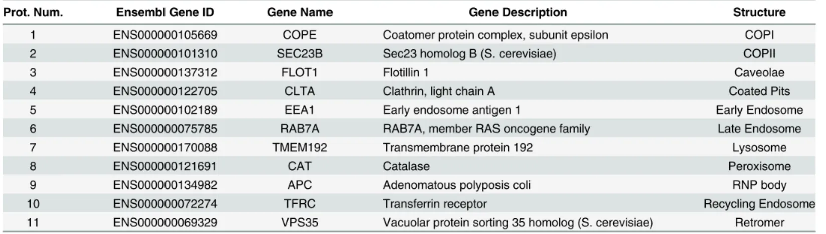
A number of proteins in the HPA are assigned annotations of“vesicles”or“cytoplasm”. We considered whether we could use HPA images to assign these proteins to a more specific organ-elle or structure. By examining UniProt annotations and primary literature for proteins whose subcellular location has been reasonably well characterized, we selected eleven proteins that are found in eleven specific types of punctate patterns (Table 1) (we refer to these proteins as “founders”since they enabled us to define specific subtypes). We chose these patterns due to the fact that the proteins showed a similar pattern across all three cell types in the HPA and they represent a wide range of membrane and non-membrane bound compartments (although there are of course additional punctate patterns for which we did not find appropriate foun-ders). In particular, they cover all main compartments of the endomembrane system. We cal-culated the feature values for all cells for each combination of the eleven proteins and three cell lines. We verified that the features accurately reflect the relationship between vesicles and microtubules by comparing the cumulative distribution of the experimentally measured dis-tance between puncta and microtubules with that calculated from the model; the distributions were very similar for all eleven patterns (S1 Fig). We then asked whether these patterns could be distinguished from each other in HPA images. To provide a visual basis for illustrating how the proteins differed in the features, we calculated the first three principal components.Fig 2onto the three most significant principal component axes, as well as the example images, it appears that the first component primarily represents variation in features 12, 13 and 5, which capture relationship to microtubules and variation in intensity. The second primarily repre-sents variation in features 21, 22, 2, and 8, which capture intensity and distance from the nucleus, while the third principal component represents variation in features 1, 3, and 4, which capture puncta size and variation in size. This figure does not permit accurate assessment of the overlap between patterns, but is presented to give a visual overview of the major modes of variation with the patterns.
Constructing a classifier for punctate subpatterns
These results suggest that the feature set may be a reliable basis for measuring variation in punctate patterns, and we therefore sought to determine whether we could use them to predict
Fig 1. (a) Summary of model learning and classification pipeline. (b) Illustration of coordinate system for probability density function. For each pixel in an image, distance between it and the nearest point on the nuclear membrane (L1) and between it and the nearest point on the cell membrane (L2) are calculated and used to calculate the radial position (r) as L1/(L1+L2). In addition, the distance to the nearest point on a segmented microtubule (d) and the angle between the pixel and the major axis of the cell (α) are calculated.
(c) A two-color image of a vesicular protein (TFRC, transferrin receptor, green) and microtubules (red) in a U-2OS cell. (d) Segmented image of microtubules (red) and puncta (green). (e) Remaining background intensity.
the compartmental localization of other proteins to one of the eleven patterns. To do this, we first used the features to construct a classification accuracy-derived separability statistic to compare two collections of cells (seeMethods) and assessed the extent to which the eleven pat-terns could be distinguished. We used a classification approach based on Bayes error rate in
Table 1. Proteins used to define punctate subpatterns in this study.
Prot. Num. Ensembl Gene ID Gene Name Gene Description Structure
1 ENS000000105669 COPE Coatomer protein complex, subunit epsilon COPI
2 ENS000000101310 SEC23B Sec23 homolog B (S. cerevisiae) COPII
3 ENS000000137312 FLOT1 Flotillin 1 Caveolae
4 ENS000000122705 CLTA Clathrin, light chain A Coated Pits
5 ENS000000102189 EEA1 Early endosome antigen 1 Early Endosome
6 ENS000000075785 RAB7A RAB7A, member RAS oncogene family Late Endosome
7 ENS000000170088 TMEM192 Transmembrane protein 192 Lysosome
8 ENS000000121691 CAT Catalase Peroxisome
9 ENS000000134982 APC Adenomatous polyposis coli RNP body
10 ENS000000072274 TFRC Transferrin receptor Recycling Endosome
11 ENS000000069329 VPS35 Vacuolar protein sorting 35 homolog (S. cerevisiae) Retromer
doi:10.1371/journal.pcbi.1004614.t001
Fig 2. Distribution of cells of the combinations of proteins and cell lines in the first three principal components learned from the whole feature space by PCA.The number for each point indicates the protein index and the color indicates the cell line (red for A-431, green for 2OS and blue for U-251MG). The gray ellipses represent the scope of 1.5 standard deviations, which contain about 50% to 80% of cells. The arrows summarize the composition of each principal component by showing the direction in which each feature increases (seeS1 Tablefor the list of features). The left panel shows the first and second principal components while the right panel shows the second and third principal components. Feature projections with a magnitude less than 0.1 were removed for visualization purposes.
order to avoid problems with imbalance between the numbers of proteins in each class and to allow for class-specific differences in scale for different features (seeMethods).
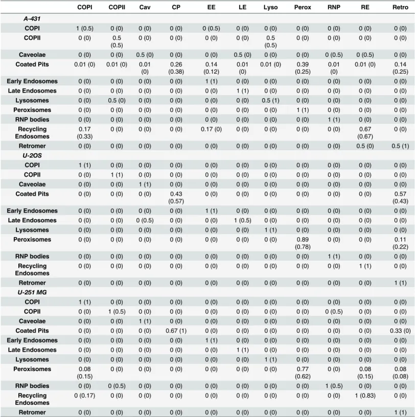
For each cell type separately, we classified each image as belonging to one of the eleven pat-terns using hold-out-image cross validation: for each held-out image, we calculated the separa-bility between the cells contained in that image and the cells of each of the founder patterns. The image was given the label of the pattern that was least separable from it. Using this method for each cell type we achieved an average class accuracy of 86.9% (Table 2). We compared these results to those using the same classification procedure but excluding the features relating to microtubule distribution, which resulted in 82.8% average accuracy. This demonstrates that the relationship to microtubules provides information that improves our ability to distinguish punctate patterns. Further examination ofTable 2reveals that the coated pits pattern is the only one that is consistently difficult to distinguish. This may in part be due to the fact that 2D confocal images were used, and thus the features cannot easily distinguish whether puncta are on the surface or inside the cell (for the other surface puncta pattern, caveolae, their distribu-tion or size must allow them to be distinguished).
Annotation of other punctate proteins
We next asked whether the classification approach could be used to assign a punctate subpat-tern annotation to an image of proteins other than the founders. We did not want to simply assign the subcellular location of the class that a protein was most similar to (since the protein might not actually be from any of our classes), but wanted to ensure that we only assigned annotations for proteins with a high degree of similarity to one of the founders. For each cell type, we determined a threshold on the separability statistic that could be used to determine whether or not a new protein should be assigned to a particular class. This threshold was deter-mined as the optimal point of the receiver operating characteristic curve (seeMethodsandS2 Fig) for each cell type.
To assign subcellular location to a new image, we measured the separability between it and each founder pattern. If the value for one of the patterns was below the threshold, we assigned the corresponding pattern label to that image. In the rare case of an image being below the threshold of multiple patterns, we assigned it the label“ambiguous.”This classification proce-dure was applied to the remainder of images in the HPA dataset; the results are contained inS1 Dataset. One hundred and twenty-five proteins were identified as belonging to one of the eleven classes in A-431, 60 in U-2OS, and 365 in U-251 MG. The list of the most confident assignments is shown inTable 3. With the goal of providing improved annotations for protein databases, we also generated an XML file that can be used to update those databases. The file (S2 Dataset) contains information on HPA antibody IDs, gene targets and proposed annota-tion. Due to the nature of immunofluorescence tagging, a sequence-specific tag may be present on more than one protein isoform, each of which may show a condition-specific localization pattern. With that in mind, we also report the known protein gene products provided by ENSEMBL 79, and the percentage of matching peptides after alignment between the gene-product and antigen sequences in the region spanned by the antibody. We also provide annota-tions to all protein isoforms that match the antibody sequence. For those proteins and isoforms that have a high confidence location assignment, we also provide an XML file for updating their UniProt record (S3 Dataset).
Table 2. Ability to distinguish 11 punctate classes.Classifiers were trained using 5-fold cross validation, and the class of the held out image was pre-dicted. Results are shown for classifiers constructed using all features, and values in parentheses are for training without the microtubule features.
COPI COPII Cav CP EE LE Lyso Perox RNP RE Retro
A-431
COPI 1 (0.5) 0 (0) 0 (0) 0 (0) 0 (0.5) 0 (0) 0 (0) 0 (0) 0 (0) 0 (0) 0 (0)
COPII 0 (0) 0.5 (0.5)
0 (0) 0 (0) 0 (0) 0 (0) 0.5
(0.5)
0 (0) 0 (0) 0 (0) 0 (0)
Caveolae 0 (0) 0 (0) 0.5 (0) 0 (0) 0 (0) 0.5 (0) 0 (0) 0 (0) 0 (0.5) 0 (0.5) 0 (0) Coated Pits 0.01 (0) 0.01 (0) 0.01
(0) 0.26 (0.38) 0.14 (0.12) 0.01 (0)
0.01 (0) 0.39 (0.25)
0.01 (0)
0.01 (0) 0.14 (0.25) Early Endosomes 0 (0) 0 (0) 0 (0) 0 (0) 1 (1) 0 (0) 0 (0) 0 (0) 0 (0) 0 (0) 0 (0)
Late Endosomes 0 (0) 0 (0) 0 (0) 0 (0) 0 (0) 1 (1) 0 (0) 0 (0) 0 (0) 0 (0) 0 (0) Lysosomes 0 (0) 0.5 (0) 0 (0) 0 (0) 0 (0) 0 (0) 0.5 (1) 0 (0) 0 (0) 0 (0) 0 (0) Peroxisomes 0 (0) 0 (0) 0 (0) 0 (0) 0 (0) 0 (0) 0 (0) 1 (1) 0 (0) 0 (0) 0 (0) RNP bodies 0 (0) 0 (0) 0 (0) 0 (0) 0 (0) 0 (0) 0 (0) 0 (0) 1 (1) 0 (0) 0 (0)
Recycling Endosomes
0.17 (0.33)
0 (0) 0 (0) 0 (0) 0.17 (0) 0 (0) 0 (0) 0 (0) 0 (0) 0.67
(0.67)
0 (0)
Retromer 0 (0) 0 (0) 0 (0) 0 (0) 0 (0) 0 (0) 0 (0) 0 (0) 0 (0) 0.5 (0) 0.5 (1)
U-2OS
COPI 1 (1) 0 (0) 0 (0) 0 (0) 0 (0) 0 (0) 0 (0) 0 (0) 0 (0) 0 (0) 0 (0)
COPII 0 (0) 1 (1) 0 (0) 0 (0) 0 (0) 0 (0) 0 (0) 0 (0) 0 (0) 0 (0) 0 (0) Caveolae 0 (0) 0 (0) 1 (1) 0 (0) 0 (0) 0 (0) 0 (0) 0 (0) 0 (0) 0 (0) 0 (0) Coated Pits 0 (0) 0 (0) 0 (0) 0.43
(0.57)
0 (0) 0 (0) 0 (0) 0 (0) 0 (0) 0 (0) 0.57
(0.43) Early Endosomes 0 (0) 0 (0) 0 (0) 0 (0) 1 (1) 0 (0) 0 (0) 0 (0) 0 (0) 0 (0) 0 (0)
Late Endosomes 0 (0) 0 (0) 0 (0.5) 0 (0) 0 (0) 1 (0.5) 0 (0) 0 (0) 0 (0) 0 (0) 0 (0) Lysosomes 0 (0) 0 (0) 0 (0) 0 (0) 0 (0) 0 (0) 1 (1) 0 (0) 0 (0) 0 (0) 0 (0) Peroxisomes 0 (0) 0 (0) 0 (0) 0 (0) 0 (0) 0 (0) 0 (0) 0.89
(0.78)
0 (0) 0 (0) 0.11
(0.22) RNP bodies 0 (0) 0 (0) 0 (0) 0 (0) 0 (0) 0 (0) 0 (0) 0 (0) 1 (1) 0 (0) 0 (0)
Recycling Endosomes
0 (0) 0 (0) 0 (0) 0 (0) 0 (0) 0 (0) 0 (0) 0 (0) 0 (0) 1 (1) 0 (0)
Retromer 0 (0) 0 (0) 0 (0) 0 (0) 0 (0) 0 (0) 0 (0) 0 (0) 0 (0) 0 (0) 1 (1)
U-251 MG
COPI 1 (1) 0 (0) 0 (0) 0 (0) 0 (0) 0 (0) 0 (0) 0 (0) 0 (0) 0 (0) 0 (0)
COPII 0 (0) 1 (0.5) 0 (0) 0 (0) 0 (0) 0 (0) 0 (0) 0 (0) 0 (0.5) 0 (0) 0 (0) Caveolae 0 (0) 0 (0) 1 (1) 0 (0) 0 (0) 0 (0) 0 (0) 0 (0) 0 (0) 0 (0) 0 (0) Coated Pits 0 (0) 0 (0) 0 (0) 0.67 (1) 0 (0) 0 (0) 0 (0) 0 (0) 0 (0) 0 (0) 0.33 (0) Early Endosomes 0 (0) 0 (0) 0 (0) 0 (0) 1 (1) 0 (0) 0 (0) 0 (0) 0 (0) 0 (0) 0 (0)
Late Endosomes 0 (0) 0 (0) 0 (0) 0 (0) 0 (0) 1 (1) 0 (0) 0 (0) 0 (0) 0 (0) 0 (0) Lysosomes 0 (0) 0 (0) 0 (0) 0 (0) 0 (0) 0 (0) 1 (1) 0 (0) 0 (0) 0 (0) 0 (0) Peroxisomes 0.08
(0.15)
0 (0) 0 (0) 0 (0) 0 (0) 0 (0) 0 (0) 0.77
(0.62)
0 (0) 0.08 (0.15)
0.08 (0.08) RNP bodies 0 (0) 0 (0.5) 0 (0) 0 (0) 0 (0) 0 (0) 0 (0) 0 (0) 1 (0.5) 0 (0) 0 (0)
Recycling Endosomes
0 (0.17) 0 (0) 0 (0) 0 (0) 0 (0) 0 (0) 0 (0) 0 (0) 0 (0) 1 (0.83) 0 (0)
Retromer 0 (0) 0 (0) 0 (0) 0 (0) 0 (0) 0 (0) 0 (0) 0 (0) 0 (0) 0 (0) 1 (1)
for A-431 cells, BRD4, has been suggested to be involved in the lysosome protolytic pathway [11]. For U-2OS, top hit RAB5C is a classic early endosomal protein [12], and prohibitin (PHB) is a multifunctional membrane protein [13] one of whose roles is in regulation of degra-dation of PAR1 [14]. For U-251MG cells, the top hits include cathepsin H (CTSH), a lysosomal enzyme, DTX3L, which regulates endosomal sorting [15], and LY6K, which, like other Ly6 antigens, is associated with glycosylphosphatidyl inositol-anchored glycoproteins (such as TEX101 [16]) that are typically found in caveolae. These findings increase our confidence in the proposed annotations.
Many of the proteins analyzed (which were all proteins assigned“vesicles”or“cytoplasm” annotations) were not assigned with high confidence to any of the 11 patterns. There are at least three potential reasons for this. First, the staining may be of low enough intensity or qual-ity that foreground cannot be adequately identified. Second, the unassigned proteins may be cytoplasmic proteins without a discernible punctate pattern, or vesicular proteins from an organelle that we have not considered. Third, they may be present in more than one of the eleven patterns, such that their pattern does not match well enough to any of them.
Table 3. Top-ranked proteins assigned to one of the ten high-confidence subpatterns.The top protein for each cell type for each subpattern (except Coated Pits) is included if its separability is less than 0.70 (which is more selective than the threshold determined inS2 Fig). The separability measures for all proteins are included inS1 Dataset.
Antibody ID
EMBL Gene ID*
Gene Name
Gene Description Proposed
Annotation
A-431
HPA017909 172113 NME6 NME/NM23 nucleoside diphosphate kinase 6 COPII
HPA007722 073417 PDE8A Phosphodiesterase 8A Caveolae
HPA038052 110013 SIAE Sialic acid acetylesterase Early Endosomes
HPA015055 141867 BRD4 Bromodomain containing 4 Lysosomes
HPA007875 149968 MMP3 Matrix metallopeptidase 3 RNP bodies
HPA029806 196305 IARS Isoleucyl-tRNA synthetase Retromer
U-2OS
HPA003220 204920 ZNF155 Zincfinger protein 155 COPII
HPA003607 100665 SERPINA4 Serpin peptidase inhibitor, clade A (alpha-1 antiproteinase, antitrypsin), member 4
Caveolae
HPA004167 108774 RAB5C Member RAS oncogene family Early Endosomes
HPA003280 167085 PHB Prohibitin Late Endosomes
HPA014907 162366 PDZK1IP1 PDZK1 interacting protein 1 Lysosomes
HPA002883 141665 FBXO15 F-box protein 15 RNP bodies
HPA010570 163840 DTX3L Deltex 3-like (Drosophila) Recycling Endosomes
HPA041566 180096 SEPT1 Septin 1 Retromer
U-251 MG
HPA023476 147174 ACRC Acidic repeat containing COPI
HPA003084 139915 MDGA2 MAM domain containing glycosylphosphatidylinositol anchor 2 COPII
HPA017770 160886 LY6K Lymphocyte antigen 6 complex, locus K Caveolae
HPA002946 004961 HCCS Holocytochrome c synthase Late Endosomes
HPA003524 103811 CTSH Cathepsin H Lysosomes
HPA015313 103034 NDRG4 NDRG family member 4 RNP bodies
*all begin with ENSG00000
Comparison of models for different patterns
Our models allow us to ask whether different punctate subclasses differ in their relationship to microtubules. We performed a simple characterization of this relationship by calculating the average actual distance of each punctum from microtubules, as well as the average distance from microtubules predicted by our fitted model.S3 Figshows a comparison of these two dis-tances for each pattern across all cell types and for each combination of pattern and cell type. A confidence interval on the average distance from microtubules was determined via the Tukey-Kramer method after two-way ANOVA [17] (across proteins and cell types). All of the symbols are quite near the diagonal, indicating that the model is in high agreement with the measure-ments. When averaged across all three cell types, retromer, recycling endosomes, and early endosomes show the closest association with microtubules, and RNP bodies, COPI vesicles and coated pits show the least. When each combination of protein and cell type is considered sepa-rately, we see greater variability in the distances (perhaps due to differences in microtubule-binding proteins or cell size or shape). COPII, lysosomes and COPI show the least variation across the three cell types, and coated pits and recycling endosomes show the greatest.
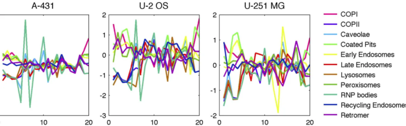
Another way in which we can compare the different patterns is by examining the differences in the model features among them. A simple visualization of this is shown inFig 3, in which the relative values of each feature are shown for each pattern. In U-2OS, for example, the first four features (relating to size and intensity) clearly distinguish the group of RNP bodies, late endosomes, recycling endosomes, lysosomes and COPII from the others, and a high value for mx5 (number of puncta) separates RNP bodies from this group. Other distinguishing features or feature combinations can also be identified, such as retromers having the lowest value for mx12 (consistent with their close association with microtubules). These differences provides a interpretable rationale for the ability of the classifiers to distinguish the patterns.
Generative model of punctate protein distributions
A difficult question that frequently gives rise to controversy is how to best describe the subcel-lular pattern of a given organelle or structure (especially a novel one). Descriptions using unstructured text or Genome Ontology terms defer the question by assuming that the words will be sufficient for the reader to be able to mentally construct the pattern. An alternative is to show an example image, but this does not give an idea of the variation in the pattern (one can find differences between any two example images, but this does not address whether those dif-ferences are statistically significant). Unfortunately these two methods of conveying informa-tion about the distribuinforma-tion and variainforma-tion in protein pattern do not provide a quantitative, or much less a probabilistic or statistical representation of the observed pattern. Alternatively, one can give values for a descriptive feature vector or matrix for each pattern (which can be used for a classifier) but this allows one only to recognize new examples but not to produce an exam-ple of the pattern. Feature vectors also do not necessarily allow an explicit model of the rela-tionship between cell components. Of course, none of the approaches above are helpful if we desire anin silicorepresentation of the cell geometry and expressed patterns (i.e., the consumer
We therefore constructed a generative model of punctate patterns whose structure is shown inFig 4. The model starts with models of nuclear and cell shape (dn, dc) and microtubule
distri-bution (dm) and links them to models of puncta distribution using mx7 through mx11 to
cap-ture dependence on cell shape and mx12 and mx13 to capcap-ture dependence on microtubules (see
Methods). Additionally the size, shape and intensity of vesicles are modeled independently of the cell shape and microtubules with mx1 through mx6. The background intensity is similarly modeled dependent on cell shape and microtubules (mx14 through 20) and scaled to match the fraction of intensity with mx21 and mx22. We illustrate that the images generated from the models learned for each of the pattern classes are similar to real images inFig 5andS4 Fig.
Assuming that the distributions of the eleven punctate patterns are independent of each other, we can combine the models and synthesize cells containing all eleven.Fig 6shows an example of a“typical”cell under this assumption (using the average values of all model parameters).
Fig 3. Comparison of model features for different patterns.The values for each feature were z-scored to put them on the same scale across features, and the average value for each feature is shown as a function of the feature number (seeS1 Tablefor feature definitions).
doi:10.1371/journal.pcbi.1004614.g003
Fig 4. Graphical model representation for the Bayesian hierarchical framework of generative model of puncta conditioned on cell geometry and microtubules.A nuclear shape is drawn from dn, a cell shape is drawn from dc, dependent on the nuclear shape [8]. A microtubule pattern is synthesized from dmdependent on the generated cell and nuclear shape [9]. The distribution of shape and positions of puncta, dp, is modeled with components pp, which models the position of puncta dependent on the cell, nucleus and microtubule pattern, and np, spand ip, which independently model the number, size and intensity of puncta. The background pattern is similarly generated dependent on the cell, nucleus and microtubule pattern with pb, and its intensity is determined with ib.
Discussion
With the development of systems to fluorescently tag and acquire images of thousands of sub-cellular protein patterns, a need arose for automated methods to analyze and model the pat-terns in these images [21]. The goals of such analyses include, but are not limited to,
Fig 5. Representative images from four patterns and corresponding synthesized images in U-2OS cells.The left column shows cell images closest to the median of parameter space for cells of that pattern, and the right column shows synthesized cells from the generative model of protein pattern conditional on cell geometry and microtubules of the left panel. The green, red and blue channels represent puncta,
microtubules and nuclei, respectively.
determining the organelles to which different proteins localize and studying the statistical dependency between different protein patterns. However, previous methods have not been able to recognize subpatterns of the major organelle types. Furthermore methods are needed to describe the relationships between cellular components in a way that is not only human-inter-pretable, but allows us to generate new examples of these patterns for future use in cell simula-tions [22].
Here we have described a new framework to build models of subcellular punctate patterns conditional on cell geometry and microtubules. These models use interpretable features that capture specific ways in which punctate subpatterns differ between cell types (such as the dif-ferences noted at the beginning of the Results) and can generate synthetic cell instances repre-sentative of the modeled population. We demonstrated the value of this framework by learning models directly from images of eleven well-characterized punctate protein patterns in three cell types. We showed that the major variation in these patterns corresponded to dependence on microtubules, total intensity, and puncta size and shape. Given the model parameters we con-structed a pipeline demonstrating both the high discriminative ability of this model across
Fig 6. Synthetic cell image containing eleven punctate patterns.Synthetic distributions for all patterns were independently created in the same cell; this assumes that positions of puncta do not affect each other (e.g., that peroxisomes are not more or less likely to be near RNP bodies). The nucleus is shown in dark grey and microtubules in light gray. Colors for patterns are the same as inFig 3.
patterns of the same cell type and the ability to automatically assign annotations to 550 pro-teins (many of which had been poorly characterized previously with respect to subcellular location).
High-content screening and analysis have become increasingly frequent, including subtle analysis of location changes induced by chemical compounds or inhibitory RNAs and prote-ome-scale analysis of patterns. The features we have described should be useful for refining the ability to distinguish different vesicular and punctate patterns, and, most importantly, to pro-vide an interpretable and portable basis for comparing them.
The work presented here represents an important step towards bridging detailed models learned from large collections of images for proteins contained in discrete objects with models of microtubule network growth learned by inverse modeling [9,18]. It serves as an important component of our CellOrganizer project (http://cellorganizer.org/) [20], which aims at captur-ing a detailed model of the spatial organization and relationships between different subcellular location patterns. We plan to extend this work by merging it with models of subcellular pattern dynamics, as well as extend the model to capture further dependency between components. It is hoped that approaches like this will enable the construction of models that capture essential cell behaviors without requiring the simultaneous measurement of the thousands of different proteins in the same living cell, something that is infeasible with current technology.
Materials and Methods
Image collections
The data used here were confocal immunofluorescence microscopy images of fixed cells from A-431, U-2OS and U-251MG cell lines from HPA [10]. All antibodies whose subcellular pat-tern was annotated as“vesicles”or“cytoplasm”were chosen (a total of 2357, 3038, and 1730 proteins for each line;S1 Datasetcontains the complete list of proteins analyzed). The images were analyzed as 8-bit TIFF images with three channels each obtained using a different emis-sion wavelength of fluorescence from a single image field. The three channels show the loca-tions of a specific punctate protein, a nuclear stain, and microtubules. Each of the images is 1728 × 1728 pixels and the pixel size corresponds to 0.08 microns in the sample plane. Founder proteins for eleven patterns were chosen as described in the Results. After segmenting the image fields for these proteins into single cell regions using a seeded watershed method [2], the set of founder images was found to contain 1099 cells, 333 from A-431, 327 from U-2OS and 439 from U-251MG (the number of cells for each of the 33combinationsof antibody and cell
line varied from 12 to 85).
Parameterization of microtubules and puncta
In cell images, due to variation in fluorescence intensity in the cytoplasm, segmentation of puncta and microtubules from protein pattern images poses a difficult problem where global threshold-based methods may over-threshold regions of the cytoplasm containing low-inten-sity structures. The input cell image was de-noised by blurring with a Gaussian filter with stan-dard deviation of 0.75. We isolated high frequency foreground and low
and all single-pixel objects. We used the skeletonized foreground signal of the microtubule image to model the distances of objects from microtubules. This approach resulted in reason-able definition of both puncta and microtubules and was sufficient to capture variation across the founder patterns analyzed in this paper.
Computing the distance between each punctum and the nearest
microtubule
The centroids of all puncta were computed by fitting a mixture of Gaussians to distinguish overlapping puncta [7]. The distance between the centroid of each punctum and its nearest microtubule was found using a distance transform of the skeletonized microtubule image.
Capturing vesicle and background position relative to microtubules and
cell and nuclear boundaries
A probability density function (PDF) for the position of puncta (pp) relative to the cell
geome-try and microtubules was estimated by extending the model previously described [8] by adding a terms describing the distance from microtubules,d:
P rð ;a;dÞ ¼
eb0þb1rþb2r 2
þb3sinaþb4cosaþb5dþb6d 2
1þeb0þb1rþb2r2þb3sinaþb4cosaþb5dþb6d2 ð1Þ
The termsβ1throughβ4describe the dependency of objects on radial and angular coordi-nates in relation to the shape of the cell [2,8], andβ5andβ6describe the dependency of objects
to be localized in relation to the microtubules. We similarly constructed a PDF for the back-ground intensity (which presumably results from soluble, non-punctate protein).
Generative models
The Bayesian hierarchical framework for the generative model for puncta is shown inFig 3as a graphical model. A multivariate statistical model was constructed from the independent distri-butions of values of the following statistics from each cell: puncta size (sp), puncta per cell (np),
and intensity (ip).
Synthetic cell instances were created starting from the cell and nuclear boundaries and microtubule image of a randomly-selected cell. (They can also be created by first generating cell and nuclear boundaries and microtubule distributions using models learned previously for the three cell lines [18].) To add puncta to a cell, values were sampled for the number of puncta per cell (np) and the size (sp) and fluorescence intensities (ip)) for each punctum from
distribu-tions learned from 2D HPA data. These were used to generate puncta using the Gaussian object based generative model [8]. Positions for them were sampled from the vesicle position PDF from the model above after morphing to the specific cell geometry. Background fluorescence was added using the learned PDF from the background images, scaled to match a draw from the total background intensity distribution learned from images.
Image classification
Given pattern parameterizations corresponding to cells of two collections (all cells con-tained in two images), we perform a balanced classification task to determine how distinguish-able the two collections are. For each pair of images, we hold out a subset of cells and train an SVM by weighting the training data such that there is a uniform prior across the classes. We then classify the hold-out and count the frequency at which the hold-out was assigned the cor-rect collection, approximating the Bayes Error rate [24]. This approach is similar to other methods used in genomics [25]. We take the average classification accuracy across all cell clas-sification tasks (whether or not the cells belonging to the two images are assigned the same sub-cellular pattern) as a measure of how distinguishable the two collections are, resulting in a possible range of values from 1 (totally separable) to 0 (completely inseparable). In virtually all cases, the measure of difference lies between 0.5 and 1. We will refer to this measure as “dissimilarity”.
To determine a threshold on dissimilarity, at which we can say two collections belong to the same or different patterns, the pipeline treats images of each of our basis patterns as their own collection (with multiple images of each pattern) and performs the above classification task using cells contained in each image. An ROC curve is constructed, indicating the true and false positive classification rates as a function of increasing dissimilarity. For each cell type we con-structed an upper-bound of dissimilarity (above which is considered“not the same annota-tion”) by the cutoff determined at the location where the upper-left-most point of the ROC curve intersects with a slope ofTNþFP
TPþFN, where TN, FP, TP and FN are the counts of true negative,
false positive, true positive and false negatives respectively. When comparing our basis set to images containing cells of unknown protein localization, we assign the unknown pattern the label of any basis pattern that is within the similarity threshold. These thresholds were 0.78846, 0.70588 and 0.72093 for A-431, U-2OS, and U-251MG, respectively.
Software availability
All software and data used for this work is available as a reproducible research archive (http:// murphylab.web.cmu.edu/software). The software will also be available as part of the open source CellOrganizer system (http://CellOrganizer.org). The segmentation and feature calcula-tion pipeline can be used separately.
Supporting Information
S1 Fig. Quality of fitted distributions for punctate proteins.P-P plots comparing the CDFs of the probability of vesicle given distance from microtubule for the fitted model and the empirical distribution are shown for the median cell of each pattern (the same cells as shown in
Fig 5andS4 Fig). (TIF)
S2 Fig. Determination of annotation threshold.Receiver operating characteristic curves for the accuracy statistic for determining the in-class threshold are shown for the three cell types. The accuracy corresponding to the optimal threshold is shown as a black circle (seeMethods). (TIF)
S3 Fig. Comparison of average distance of puncta from microtubules measured empirically and in our fitted model across proteins, cell types, and proteins and cell types.Each symbol represents a cell type; square for A-431, diamond for U-2 OS and circle for U-251 MG. The lines represent confidence intervals using Tukey’s range test for the empirical data (x-axis) and fitted model (y-axis) after 2-way ANOVA.
S4 Fig. Representative images from seven patterns and corresponding synthesized protein pattern in U-2OS cells.The left column shows cell images closest to the median of parameter space for cells of that pattern, and the right column shows synthesized protein patterns from the generative model of protein pattern conditional on cell geometry and microtubules of the left panel.
(TIF)
S1 Dataset. Results for comparison of HPA proteins to the eleven punctate subpattern clas-ses.The values in the columns for each subpattern are the separability measures for all cells of a given protein with the cells of the founder protein(s) for that subpattern.
(XLS)
S2 Dataset. Updated protein annotations resulting from this work.The file is in XML for-mat appropriate for incorporation into protein databases. These entries are only for those pro-teins assigned to a single pattern using the thresholds determined inS2 Fig.
(XML)
S3 Dataset. Updated protein annotations for the UniProt database.The information inS2 Datasetis reformatted and includes Genome Ontology terms to be assigned to each protein. (XML)
S1 Table. Generative model parameters.Radial position is defined asr=L1/(L1+L2) where L1 is the distance between the center of each punctum and the nuclear membrane, andL2 is
the distance from the center of each punctum to the cell membrane. Therefore,ris positive if
the punctum is outside of the nucleus and negative inside.αis the angle between the major axis of the cell and the vector from the center of cell to the center of a punctum. The generative model component that a given feature is used for is also shown (seeFig 3).
(DOCX)
Acknowledgments
We thank the Human Protein Atlas project, especially Devin Sullivan and Emma Lundberg, for providing images, and members of the Rohde and Murphy groups, especially Ivan Cao-Berg and Armaghan W. Naik, for their assistance and helpful comments.
Author Contributions
Conceived and designed the experiments: GRJ JL AS GKR RFM. Performed the experiments: GRJ JL AS. Analyzed the data: GRJ JL AS GKR RFM. Wrote the paper: GRJ JL AS GKR RFM.
References
1. Murphy RF, Velliste M, Porreca G. Robust numerical features for description and classification of sub-cellular location patterns in fluorescence microscope images. J VLSI Sig Proc. 2003; 35(3):311–21. 2. Li J, Newberg JY, Uhlen M, Lundberg E, Murphy RF. Automated analysis and reannotation of
subcellu-lar locations in confocal images from the Human Protein Atlas. PloS one. 2012; 7(11):e50514. Epub 2012/12/12. doi:10.1371/journal.pone.0050514PMID:23226299; PubMed Central PMCID: PMC3511558.
3. Bloom GS, Goldstein LS. Cruising along microtubule highways: how membranes move through the secretory pathway. J Cell Biol. 1998; 140(6):1277–80. PMID:9508761; PubMed Central PMCID: PMCPMC2132669.
4. Moraru II, Schaff JC, Slepchenko BM, Loew LM. The virtual cell: an integrated modeling environment for experimental and computational cell biology. Ann N Y Acad Sci. 2002; 971:595–6. PMID:12438191. 5. Tomita M, Hashimoto K, Takahashi K, Shimizu TS, Matsuzaki Y, Miyoshi F, et al. E-CELL: software
6. Kerr RA, Bartol TM, Kaminsky B, Dittrich M, Chang JC, Baden SB, et al. Fast Monte Carlo Simulation Methods for Biological Reaction-Diffusion Systems in Solution and on Surfaces. SIAM J Sci Comput. 2008; 30(6):3126. doi:10.1137/070692017PMID:20151023; PubMed Central PMCID: PMC2819163. 7. Zhao T, Murphy RF. Automated learning of generative models for subcellular location: building blocks
for systems biology. Cytometry Part A. 2007; 71A(12):978–90. PMID:17972315.
8. Peng T, Murphy RF. Image-derived, Three-dimensional Generative Models of Cellular Organization. Cytometry Part A. 2011; 79A:383–91.
9. Shariff A, Murphy RF, Rohde GK. A generative model of microtubule distributions, and indirect estima-tion of its parameters from fluorescence microscopy images. Cytometry Part A. 2010; 77A(5):457–66. Epub 2010/01/28. doi:10.1002/cyto.a.20854PMID:20104579.
10. Barbe L, Lundberg E, Oksvold P, Stenius A, Lewin E, Bjorling E, et al. Toward a confocal subcellular atlas of the human proteome. Mol Cell Proteomics. 2008; 7(3):499–508. Epub 2007/11/22. doi:10. 1074/mcp.M700325-MCP200PMID:18029348.
11. Schulze J, Moosmayer D, Weiske J, Fernandez-Montalvan A, Herbst C, Jung M, et al. Cell-based pro-tein stabilization assays for the detection of interactions between small-molecule inhibitors and BRD4. J Biomol Screen. 2015; 20(2):180–9. doi:10.1177/1087057114552398PMID:25266565.
12. Bucci C, Parton RG, Mather IH, Stunnenberg H, Simons K, Hoflack B, et al. The small GTPase rab5 func-tions as a regulatory factor in the early endocytic pathway. Cell. 1992; 70(5):715–28. PMID:1516130. 13. Mishra S, Murphy LC, Murphy LJ. The Prohibitins: emerging roles in diverse functions. J Cell Mol Med.
2006; 10(2):353–63. PMID:16796804; PubMed Central PMCID: PMCPMC3933126.
14. Wang YJ, Guo XL, Li SA, Zhao YQ, Liu ZC, Lee WH, et al. Prohibitin is involved in the activated internal-ization and degradation of protease-activated receptor 1. Biochimica et biophysica acta. 2014; 1843 (7):1393–401. doi:10.1016/j.bbamcr.2014.04.005PMID:24732013.
15. Holleman J, Marchese A. The ubiquitin ligase deltex-3l regulates endosomal sorting of the G protein-coupled receptor CXCR4. Mol Biol Cell. 2014; 25(12):1892–904. doi:10.1091/mbc.E13-10-0612
PMID:24790097; PubMed Central PMCID: PMCPMC4055268.
16. Yoshitake H, Tsukamoto H, Maruyama-Fukushima M, Takamori K, Ogawa H, Araki Y. TEX101, a germ cell-marker glycoprotein, is associated with lymphocyte antigen 6 complex locus k within the mouse testis. Biochem Biophys Res Commun. 2008; 372(2):277–82. doi:10.1016/j.bbrc.2008.05.088PMID:
18503752.
17. Tukey JW. Comparing individual means in the analysis of variance. Biometrics. 1949; 5(2):99–114. PMID:18151955.
18. Li J, Shariff A, Wiking M, Lundberg E, Rohde GK, Murphy RF. Estimating microtubule distributions from 2D immunofluorescence microscopy images reveals differences among human cultured cell lines. PloS one. 2012; 7(11):e50292. Epub 2012/12/05. doi:10.1371/journal.pone.0050292PMID:
23209697; PubMed Central PMCID: PMC3508979.
19. Buck TE, Li J, Rohde GK, Murphy RF. Toward the virtual cell: automated approaches to building mod-els of subcellular organization "learned" from microscopy images. BioEssays: news and reviews in molecular, cellular and developmental biology. 2012; 34(9):791–9. Epub 2012/07/11. doi:10.1002/ bies.201200032PMID:22777818; PubMed Central PMCID: PMC3428744.
20. Murphy RF. CellOrganizer: Image-derived Models of Subcellular Organization and Protein Distribution. Methods in cell biology. 2012; 110:179–93. doi:10.1016/B978-0-12-388403-9.00007-2PMID:22482949
21. Boland MV, Markey MK, Murphy RF. Automated recognition of patterns characteristic of subcellular structures in fluorescence microscopy images. Cytometry. 1998; 33(3):366–75. PMID:9822349
22. Sullivan DP, Arepally R, Murphy RF, Tapia J-J, Faeder JR, Dittrich M, et al. Design Automation for Bio-logical Models: A Pipeline that Incorporates Spatial and Molecular Complexity. Proceedings of the 25th edition on Great Lakes Symposium on VLSI; Pittsburgh, Pennsylvania, USA. 2743763: ACM; 2015. p. 321–3.
23. Ridler TW, Calvard S. Picture thresholding using an iterative selection method. IEEE Trans Syst Man Cybernet. 1978; SMC-8(8):630–2.
24. Tumer K, Ghosh J, editors. Estimating the Bayes error rate through classifier combining. Pattern Rec-ognition, 1996, Proceedings of the 13th International Conference on; 1996 25–29 Aug 1996. 25. Zhang JG, Deng HW. Gene selection for classification of microarray data based on the Bayes error.