Mathematical Biology, II. Spatial Models and Biomedical Applications.

II: Spatial Models and

Biomedical Applications,

Third Edition

J. D. Murray

Volume 18

Editors

S.S. Antman J.E. Marsden L. Sirovich S. Wiggins

Geophysics and Planetary Sciences Mathematical Biology

L. Glass, J.D. Murray

Mechanics and Materials R.V. Kohn

Systems and Control

S.S. Sastry, P.S. Krishnaprasad

Problems in engineering, computational science, and the physical and biological sci-ences are using increasingly sophisticated mathematical techniques. Thus, the bridge between the mathematical sciences and other disciplines is heavily traveled. The corre-spondingly increased dialog between the disciplines has led to the establishment of the series:Interdisciplinary Applied Mathematics.

The purpose of this series is to meet the current and future needs for the interaction between various science and technology areas on the one hand and mathematics on the other. This is done, firstly, by encouraging the ways that mathematics may be applied in traditional areas, as well as point towards new and innovative areas of applications; and secondly, by encouraging other scientific disciplines to engage in a dialog with mathe-maticians outlining their problems to both access new methods and suggest innovative developments within mathematics itself.

Volumes published are listed at the end of the book.

Springer

Mathematical Biology

II: Spatial Models and

Biomedical Applications

Third Edition

With 298 Illustrations

University of Oxfordand University of Washington Box 352420

Department of Applied Mathematics Seattle, WA 98195-2420

USA

Editors

S.S. Antman J.E. Marsden

Department of Mathematics Control and Dynamical Systems andInstitute for Physical Science Mail Code 107-81

and Technology California Institute of Technology

University of Maryland Pasadena, CA 91125

College Park, MD 20742-4015 USA

USA marsden@cds.caltech.edu

ssa@math.umd.edu

L. Sirovich S. Wiggins

Division of Applied Mathematics School of Mathematics

Brown University University of Bristol

Providence, RI 02912 Bristol BS8 1TW

USA UK

chico@camelot.mssm.edu s.wiggins@bris.ac.uk

Cover illustration: cAlain Pons.

Mathematics Subject Classification (2000): 92B05, 92-01, 92C05, 92D30, 34Cxx

Library of Congress Cataloging-in-Publication Data Murray, J.D. (James Dickson)

Mathematical biology. II: Spatial models and biomedical applications / J.D. Murray.—3rd ed. p. cm.—(Interdisciplinary applied mathematics)

Rev. ed. of: Mathematical biology. 2nd ed. c1993. Includes bibliographical references (p. ). ISBN 0-387-95228-4 (alk. paper)

1. Biology—Mathematical models. I. Murray, J.D. (James Dickson) Mathematical biology. II. Title. III. Series.

QH323.5 .M88 2001b

570′.1′5118—dc21 2001020447

ISBN 0-387-95228-4 Printed on acid-free paper.

c

2003 J.D. Murray, c1989, 1993 Springer-Verlag Berlin Heidelberg.

All rights reserved. This work may not be translated or copied in whole or in part without the written per-mission of the publisher (Springer-Verlag New York, Inc., 175 Fifth Avenue, New York, NY 10010, USA), except for brief excerpts in connection with reviews or scholarly analysis. Use in connection with any form of information storage and retrieval, electronic adaptation, computer software, or by similar or dissimilar methodology now known or hereafter developed is forbidden.

The use in this publication of trade names, trademarks, service marks, and similar terms, even if they are not identified as such, is not to be taken as an expression of opinion as to whether or not they are subject to proprietary rights.

Printed in the United States of America.

9 8 7 6 5 4 3 2 1 SPIN 10792366

www.springer-ny.com

Springer-Verlag New York Berlin Heidelberg

general criaci´on del mundo, i de lo que en ´el se

encierra, i se hall´a ra con ´el, se huvieran

producido

i formado algunas cosas mejor que fueran hechas,

i otras ni se hicieran, u se enmendaran i corrigieran.

Alphonso X (Alphonso the Wise), 1221–1284 King of Castile and Leon (attributed)

In the thirteen years since the first edition of this book appeared the growth of mathe-matical biology and the diversity of applications has been astonishing. Its establishment as a distinct discipline is no longer in question. One pragmatic indication is the in-creasing number of advertised positions in academia, medicine and industry around the world; another is the burgeoning membership of societies. People working in the field now number in the thousands. Mathematical modelling is being applied in every ma-jor discipline in the biomedical sciences. A very different application, and surprisingly successful, is in psychology such as modelling various human interactions, escalation to date rape and predicting divorce.

The field has become so large that, inevitably, specialised areas have developed which are, in effect, separate disciplines such as biofluid mechanics, theoretical ecology and so on. It is relevant therefore to ask why I felt there was a case for a new edition of a book called simplyMathematical Biology. It is unrealistic to think that a single book could cover even a significant part of each subdiscipline and this new edition certainly does not even try to do this. I feel, however, that there is still justification for a book which can demonstrate to the uninitiated some of the exciting problems that arise in biology and give some indication of the wide spectrum of topics that modelling can address.

In many areas the basics are more or less unchanged but the developments during the past thirteen years have made it impossible to give as comprehensive a picture of the current approaches in and the state of the field as was possible in the late 1980s. Even then important areas were not included such as stochastic modelling, biofluid mechanics and others. Accordingly in this new edition only some of the basic modelling concepts are discussed—such as in ecology and to a lesser extent epidemiology—but references are provided for further reading. In other areas recent advances are discussed together with some new applications of modelling such as in marital interaction (Volume I), growth of cancer tumours (Volume II), temperature-dependent sex determination (Vol-ume I) and wolf territoriality (Vol(Vol-ume II). There have been many new and fascinating developments that I would have liked to include but practical space limitations made it impossible and necessitated difficult choices. I have tried to give some idea of the diversity of new developments but the choice is inevitably prejudiced.

possible to relate the mathematical models to specific experiments or even biological entities. Nevertheless such an approach has spawned numerous experiments based as much on the modelling approach as on the actual mechanism studied. Some of the more mathematical parts in which the biological connection was less immediate have been excised while others that have been kept have a mathematical and technical pedagogical aim but all within the context of their application to biomedical problems. I feel even more strongly about the philosophy of mathematical modelling espoused in the original preface as regards what constitutes good mathematical biology. One of the most exciting aspects regarding the new chapters has been their genuine interdisciplinary collaborative character. Mathematical or theoretical biology is unquestionably an interdisciplinary sciencepar excellence.

The unifying aim of theoretical modelling and experimental investigation in the biomedical sciences is the elucidation of the underlying biological processes that re-sult in a particular observed phenomenon, whether it is pattern formation in develop-ment, the dynamics of interacting populations in epidemiology, neuronal connectivity and information processing, the growth of tumours, marital interaction and so on. I must stress, however, that mathematical descriptions of biological phenomena are not biological explanations. The principal use of any theory is in its predictions and, even though different models might be able to create similar spatiotemporal behaviours, they are mainly distinguished by the different experiments they suggest and, of course, how closely they relate to the real biology. There are numerous examples in the book.

Why use mathematics to study something as intrinsically complicated and ill un-derstood as development, angiogenesis, wound healing, interacting population dynam-ics, regulatory networks, marital interaction and so on? We suggest that mathematdynam-ics, rather theoretical modelling, must be used if we ever hope to genuinely and realistically convert an understanding of the underlying mechanisms into a predictive science. Math-ematics is required to bridge the gap between the level on which most of our knowledge is accumulating (in developmental biology it is cellular and below) and the macroscopic level of the patterns we see. In wound healing and scar formation, for example, a mathe-matical approach lets us explore the logic of the repair process. Even if the mechanisms were well understood (and they certainly are far from it at this stage) mathematics would be required to explore the consequences of manipulating the various parameters asso-ciated with any particular scenario. In the case of such things as wound healing and cancer growth—and now in angiogensesis with its relation to possible cancer therapy— the number of options that are fast becoming available to wound and cancer managers will become overwhelming unless we can find a way to simulate particular treatment protocols before applying them in practice. The latter has been already of use in under-standing the efficacy of various treatment scenarios with brain tumours (glioblastomas) and new two step regimes for skin cancer.

In development (by way of example) it is true that we are a long way from be-ing able to reliably simulate actual biological development, in spite of the plethora of models and theory that abound. Key processes are generally still poorly understood. Despite these limitations, I feel that exploring the logic of pattern formation is worth-while, or rather essential, even in our present state of knowledge. It allows us to take a hypothetical mechanism and examine its consequences in the form of a mathemat-ical model, make predictions and suggest experiments that would verify or invalidate the model; even the latter casts light on the biology. The very process of constructing a mathematical model can be useful in its own right. Not only must we commit to a particular mechanism, but we are also forced to consider what is truly essential to the process, the central players (variables) and mechanisms by which they evolve. We are thus involved in constructing frameworks on which we can hang our understanding. The model equations, the mathematical analysis and the numerical simulations that follow serve to reveal quantitatively as well as qualitatively the consequences of that logical structure.

This new edition is published in two volumes. Volume I is an introduction to the field; the mathematics mainly involves ordinary differential equations but with some basic partial differential equation models and is suitable for undergraduate and graduate courses at different levels. Volume II requires more knowledge of partial differential equations and is more suitable for graduate courses and reference.

I would like to acknowledge the encouragement and generosity of the many peo-ple who have written to me (including a prison inmate in New England) since the ap-pearance of the first edition of this book, many of whom took the trouble to send me details of errors, misprints, suggestions for extending some of the models, suggesting collaborations and so on. Their input has resulted in many successful interdisciplinary research projects several of which are discussed in this new edition. I would like to thank my colleagues Mark Kot and Hong Qian, many of my former students, in partic-ular Patricia Burgess, Julian Cook, Trac´e Jackson, Mark Lewis, Philip Maini, Patrick Nelson, Jonathan Sherratt, Kristin Swanson and Rebecca Tyson for their advice or care-ful reading of parts of the manuscript. I would also like to thank my former secretary Erik Hinkle for the care, thoughtfulness and dedication with which he put much of the manuscript into LA_{TEX and his general help in tracking down numerous obscure}

refer-ences and material.

and informative model is a talent I have tried to acquire throughout my career. Finally, although it is not possible to thank by name all of my past students, postdoctorals, nu-merous collaborators and colleagues around the world who have encouraged me in this field, I am certainly very much in their debt.

Looking back on my involvement with mathematics and the biomedical sciences over the past nearly thirty years my major regret is that I did not start working in the field years earlier.

Bainbridge Island, Washington J.D. Murray

Mathematics has always benefited from its involvement with developing sciences. Each successive interaction revitalises and enhances the field. Biomedical science is clearly the premier science of the foreseeable future. For the continuing health of their subject, mathematicians must become involved with biology. With the example of how mathe-matics has benefited from and influenced physics, it is clear that if mathematicians do not become involved in the biosciences they will simply not be a part of what are likely to be the most important and exciting scientific discoveries of all time.

Mathematical biology is a fast-growing, well-recognised, albeit not clearly defined, subject and is, to my mind, the most exciting modern application of mathematics. The increasing use of mathematics in biology is inevitable as biology becomes more quan-titative. The complexity of the biological sciences makes interdisciplinary involvement essential. For the mathematician, biology opens up new and exciting branches, while for the biologist, mathematical modelling offers another research tool commensurate with a new powerful laboratory technique butonlyif used appropriately and its limitations recognised. However, the use of esoteric mathematics arrogantly applied to biologi-cal problems by mathematicians who know little about the real biology, together with unsubstantiated claims as to how important such theories are, do little to promote the interdisciplinary involvement which is so essential.

Mathematical biology research, to be useful and interesting, must be relevant bio-logically. The best models show how a process works and then predict what may fol-low. If these are not already obvious to the biologistsandthe predictions turn out to be right, then you will have the biologists’ attention. Suggestions as to what the governing mechanisms are may evolve from this.Genuineinterdisciplinary research and the use of models can produce exciting results, many of which are described in this book.

No previous knowledge of biology is assumed of the reader. With each topic dis-cussed I give a brief description of the biological background sufficient to understand the models studied. Although stochastic models are important, to keep the book within reasonable bounds, I deal exclusively with deterministic models. The book provides a toolkit of modelling techniques with numerous examples drawn from population ecol-ogy, reaction kinetics, biological oscillators, developmental biolecol-ogy, evolution, epidemi-ology and other areas.

un-informed use of models. I hope the reader will acquire a practical and realistic view of biological modelling and the mathematical techniques needed to get approximate quantitative solutions and will thereby realise the importance of relating the models and results to the real biological problems under study. If the use of a model stimulates experiments—even if the model is subsequently shown to be wrong—then it has been successful. Models can provide biological insight and be very useful in summarising, interpreting and interpolating real data. I hope the reader will also learn that (certainly at this stage) there is usually no ‘right’ model: producing similar temporal or spatial pat-terns to those experimentally observed is only a first step and does not imply the model mechanism is the one which applies. Mathematical descriptions arenotexplanations. Mathematics can never provide the complete solution to a biological problem on its own. Modern biology is certainly not at the stage where it is appropriate for mathemati-cians to try to construct comprehensive theories. A close collaboration with biologists is needed for realism, stimulation and help in modifying the model mechanisms to reflect the biology more accurately.

Although this book is titled mathematical biologyit is not, and could not be, a definitive all-encompassing text. The immense breadth of the field necessitates a re-stricted choice of topics. Some of the models have been deliberately kept simple for pedagogical purposes. The exclusion of a particular topic—population genetics, for example—in no way reflects my view as to its importance. However, I hope the range of topics discussed will show how exciting intercollaborative research can be and how significant a role mathematics can play. The main purpose of the book is to present some of the basic and, to a large extent, generally accepted theoretical frameworks for a variety of biological models. The material presented does not purport to be the latest de-velopments in the various fields, many of which are constantly expanding. The already lengthy list of references is by no means exhaustive and I apologise for the exclusion of many that should be included in a definitive list.

With the specimen models discussed and the philosophy which pervades the book, the reader should be in a position to tackle the modelling of genuinely practical prob-lems with realism. From amathematicalpoint of view, the art of good modelling relies on: (i) a sound understanding and appreciation of the biological problem; (ii) a realistic mathematical representation of the important biological phenomena; (iii) finding use-ful solutions, preferably quantitative; and what is crucially important; (iv) a biological interpretation of the mathematical results in terms of insights and predictions. The math-ematics is dictated by the biology and not vice versa. Sometimes the mathmath-ematics can be very simple. Useful mathematical biology research is not judged by mathematical standards but by different and no less demanding ones.

valuable suggestions and kindly provided me with photographs. I would particularly like to thank Drs. Philip Maini, David Lane, and Diana Woodward and my present graduate students who read various drafts with such care, specifically Daniel Bentil, Meghan Burke, David Crawford, Michael Jenkins, Mark Lewis, Gwen Littlewort, Mary Myerscough, Katherine Rogers and Louisa Shaw.

Oxford J.D. Murray

CONTENTS, VOLUME II

Preface to the Third Edition vii

Preface to the First Edition xi

1. Multi-Species Waves and Practical Applications 1

1.1 Intuitive Expectations . . . 1

1.2 Waves of Pursuit and Evasion in Predator–Prey Systems . . . 5

1.3 Competition Model for the Spatial Spread of the Grey Squirrel in Britain . . . 12

1.4 Spread of Genetically Engineered Organisms . . . 18

1.5 Travelling Fronts in the Belousov–Zhabotinskii Reaction . . . 35

1.6 Waves in Excitable Media . . . 41

1.7 Travelling Wave Trains in Reaction Diffusion Systems with Oscillatory Kinetics . . . 49

1.8 Spiral Waves . . . 54

1.9 Spiral Wave Solutions ofλ–ωReaction Diffusion Systems . . . 61

Exercises . . . 67

2. Spatial Pattern Formation with Reaction Diffusion Systems 71 2.1 Role of Pattern in Biology . . . 71

2.2 Reaction Diffusion (Turing) Mechanisms . . . 75

2.3 General Conditions for Diffusion-Driven Instability: Linear Stability Analysis and Evolution of Spatial Pattern . . . 82

2.4 Detailed Analysis of Pattern Initiation in a Reaction Diffusion Mechanism . . . 90

2.5 Dispersion Relation, Turing Space, Scale and Geometry Effects in Pattern Formation Models . . . 103

2.6 Mode Selection and the Dispersion Relation . . . 113

2.8 Spatial Patterns in Scalar Population Interaction Diffusion

Equations with Convection: Ecological Control Strategies . . . 125

2.9 Nonexistence of Spatial Patterns in Reaction Diffusion Systems: General and Particular Results . . . 130

Exercises . . . 135

3. Animal Coat Patterns and Other Practical Applications of Reaction Diffusion Mechanisms 141 3.1 Mammalian Coat Patterns—‘How the Leopard Got Its Spots’ . . . 142

3.2 Teratologies: Examples of Animal Coat Pattern Abnormalities . . . . 156

3.3 A Pattern Formation Mechanism for Butterfly Wing Patterns . . . 161

3.4 Modelling Hair Patterns in a Whorl inAcetabularia . . . 180

4. Pattern Formation on Growing Domains: Alligators and Snakes 192 4.1 Stripe Pattern Formation in the Alligator: Experiments . . . 193

4.2 Modelling Concepts: Determining the Time of Stripe Formation . . . 196

4.3 Stripes and Shadow Stripes on the Alligator . . . 200

4.4 Spatial Patterning of Teeth Primordia in the Alligator: Background and Relevance . . . 205

4.5 Biology of Tooth Initiation . . . 207

4.6 Modelling Tooth Primordium Initiation: Background . . . 213

4.7 Model Mechanism for Alligator Teeth Patterning . . . 215

4.8 Results and Comparison with Experimental Data . . . 224

4.9 Prediction Experiments . . . 228

4.10 Concluding Remarks on Alligator Tooth Spatial Patterning . . . 232

4.11 Pigmentation Pattern Formation on Snakes . . . 234

4.12 Cell-Chemotaxis Model Mechanism . . . 238

4.13 Simple and Complex Snake Pattern Elements . . . 241

4.14 Propagating Pattern Generation with the Cell-Chemotaxis System . . 248

5. Bacterial Patterns and Chemotaxis 253 5.1 Background and Experimental Results . . . 253

5.2 Model Mechanism forE. coliin the Semi-Solid Experiments . . . 260

5.3 Liquid Phase Model: Intuitive Analysis of Pattern Formation . . . 267

5.4 Interpretation of the Analytical Results and Numerical Solutions . . . 274

5.5 Semi-Solid Phase Model Mechanism forS. typhimurium . . . 279

5.6 Linear Analysis of the Basic Semi-Solid Model . . . 281

5.7 Brief Outline and Results of the Nonlinear Analysis . . . 287

5.8 Simulation Results, Parameter Spaces and Basic Patterns . . . 292

5.9 Numerical Results with Initial Conditions from the Experiments . . . 297

5.10 Swarm Ring Patterns with the Semi-Solid Phase Model Mechanism . 299 5.11 Branching Patterns inBacillus subtilis . . . 306

6.2 Mechanical Model for Mesenchymal Morphogenesis . . . 319

6.3 Linear Analysis, Dispersion Relation and Pattern Formation Potential . . . 330

6.4 Simple Mechanical Models Which Generate Spatial Patterns with Complex Dispersion Relations . . . 334

6.5 Periodic Patterns of Feather Germs . . . 345

6.6 Cartilage Condensations in Limb Morphogenesis and Morphogenetic Rules . . . 350

6.7 Embryonic Fingerprint Formation . . . 358

6.8 Mechanochemical Model for the Epidermis . . . 367

6.9 Formation of Microvilli . . . 374

6.10 Complex Pattern Formation and Tissue Interaction Models . . . 381

Exercises . . . 394

7. Evolution, Morphogenetic Laws, Developmental Constraints and Teratologies 396 7.1 Evolution and Morphogenesis . . . 396

7.2 Evolution and Morphogenetic Rules in Cartilage Formation in the Vertebrate Limb . . . 402

7.3 Teratologies (Monsters) . . . 407

7.4 Developmental Constraints, Morphogenetic Rules and the Consequences for Evolution . . . 411

8. A Mechanical Theory of Vascular Network Formation 416 8.1 Biological Background and Motivation . . . 416

8.2 Cell–Extracellular Matrix Interactions for Vasculogenesis . . . 417

8.3 Parameter Values . . . 425

8.4 Analysis of the Model Equations . . . 427

8.5 Network Patterns: Numerical Simulations and Conclusions . . . 433

9. Epidermal Wound Healing 441 9.1 Brief History of Wound Healing . . . 441

9.2 Biological Background: Epidermal Wounds . . . 444

9.3 Model for Epidermal Wound Healing . . . 447

9.4 Nondimensional Form, Linear Stability and Parameter Values . . . 450

9.5 Numerical Solution for the Epidermal Wound Repair Model . . . 451

9.6 Travelling Wave Solutions for the Epidermal Model . . . 454

9.7 Clinical Implications of the Epidermal Wound Model . . . 461

9.8 Mechanisms of Epidermal Repair in Embryos . . . 468

9.9 Actin Alignment in Embryonic Wounds: A Mechanical Model . . . . 471

9.10 Mechanical Model with Stress Alignment of the Actin Filaments in Two Dimensions . . . 482

10.2 Logic of Wound Healing and Initial Models . . . 495

10.3 Brief Review of Subsequent Developments . . . 500

10.4 Model for Fibroblast-Driven Wound Healing: Residual Strain and Tissue Remodelling . . . 503

10.5 Solutions of the Model Equations and Comparison with Experiment . . . 507

10.6 Wound Healing Model of Cook (1995) . . . 511

10.7 Matrix Secretion and Degradation . . . 515

10.8 Cell Movement in an Oriented Environment . . . 518

10.9 Model System for Dermal Wound Healing with Tissue Structure . . . 521

10.10 One-Dimensional Model for the Structure of Pathological Scars . . . 526

10.11 Open Problems in Wound Healing . . . 530

10.12 Concluding Remarks on Wound Healing . . . 533

11. Growth and Control of Brain Tumours 536 11.1 Medical Background . . . 538

11.2 Basic Mathematical Model of Glioma Growth and Invasion . . . 542

11.3 Tumour SpreadIn Vitro: Parameter Estimation . . . 550

11.4 Tumour Invasion in the Rat Brain . . . 559

11.5 Tumour Invasion in the Human Brain . . . 563

11.6 Modelling Treatment Scenarios: General Comments . . . 579

11.7 Modelling Tumour Resection in Homogeneous Tissue . . . 580

11.8 Analytical Solution for Tumour Recurrence After Resection . . . 584

11.9 Modelling Surgical Resection with Brain Tissue Heterogeneity . . . . 588

11.10 Modelling the Effect of Chemotherapy on Tumour Growth . . . 594

11.11 Modelling Tumour Polyclonality and Cell Mutation . . . 605

12. Neural Models of Pattern Formation 614 12.1 Spatial Patterning in Neural Firing with a Simple Activation–Inhibition Model . . . 614

12.2 A Mechanism for Stripe Formation in the Visual Cortex . . . 622

12.3 A Model for the Brain Mechanism Underlying Visual Hallucination Patterns . . . 627

12.4 Neural Activity Model for Shell Patterns . . . 638

12.5 Shamanism and Rock Art . . . 655

Exercises . . . 659

13. Geographic Spread and Control of Epidemics 661 13.1 Simple Model for the Spatial Spread of an Epidemic . . . 661

13.2 Spread of the Black Death in Europe 1347–1350 . . . 664

13.3 Brief History of Rabies: Facts and Myths . . . 669

13.4 The Spatial Spread of Rabies Among Foxes I: Background and Simple Model . . . 673

13.6 Control Strategy Based on Wave Propagation into a

Nonepidemic Region: Estimate of Width of a Rabies Barrier . . . 696 13.7 Analytic Approximation for the Width of the Rabies

Control Break . . . 700 13.8 Two-Dimensional Epizootic Fronts and Effects of Variable Fox

Densities: Quantitative Predictions for a Rabies Outbreak

in England . . . 704 13.9 Effect of Fox Immunity on the Spatial Spread of Rabies . . . 710 Exercises . . . 720 14. Wolf Territoriality, Wolf–Deer Interaction and Survival 722 14.1 Introduction and Wolf Ecology . . . 722 14.2 Models for Wolf Pack Territory Formation:

Single Pack—Home Range Model . . . 729 14.3 Multi-Wolf Pack Territorial Model . . . 734 14.4 Wolf–Deer Predator–Prey Model . . . 745 14.5 Concluding Remarks on Wolf Territoriality and Deer Survival . . . . 751 14.6 Coyote Home Range Patterns . . . 753 14.7 Chippewa and Sioux Intertribal Conflict c1750–1850 . . . 754 Appendix

A. General Results for the Laplacian Operator in Bounded Domains 757

Bibliography 761

CONTENTS, VOLUME I

J.D. Murray: Mathematical Biology, I: An Introduction

Preface to the Third Edition vii

Preface to the First Edition xi

3.3 Realistic Predator–Prey Models . . . 86 3.4 Analysis of a Predator–Prey Model with Limit Cycle

Periodic Behaviour: Parameter Domains of Stability . . . 88 3.5 Competition Models: Competitive Exclusion Principle . . . 94 3.6 Mutualism or Symbiosis . . . 99 3.7 General Models and Cautionary Remarks . . . 101 3.8 Threshold Phenomena . . . 105 3.9 Discrete Growth Models for Interacting Populations . . . 109 3.10 Predator–Prey Models: Detailed Analysis . . . 110 Exercises . . . 115 4. Temperature-Dependent Sex Determination (TSD) 119 4.1 Biological Introduction and Historical Asides on the Crocodilia . . . . 119 4.2 Nesting Assumptions and Simple Population Model . . . 124 4.3 Age-Structured Population Model for Crocodilia . . . 130 4.4 Density-Dependent Age-Structured Model Equations . . . 133 4.5 Stability of the Female Population in Wet Marsh Region I . . . 135 4.6 Sex Ratio and Survivorship . . . 137 4.7 Temperature-Dependent Sex Determination (TSD) Versus

Genetic Sex Determination (GSD) . . . 139 4.8 Related Aspects on Sex Determination . . . 142 Exercise . . . 144 5. Modelling the Dynamics of Marital Interaction: Divorce Prediction

and Marriage Repair 146

5.1 Psychological Background and Data:

Gottman and Levenson Methodology . . . 147 5.2 Marital Typology and Modelling Motivation . . . 150 5.3 Modelling Strategy and the Model Equations . . . 153 5.4 Steady States and Stability . . . 156 5.5 Practical Results from the Model . . . 164 5.6 Benefits, Implications and Marriage Repair Scenarios . . . 170

6. Reaction Kinetics 175

7.3 Oscillators and Switches with Two or More Species:

General Qualitative Results . . . 226 7.4 Simple Two-Species Oscillators: Parameter Domain

Determination for Oscillations . . . 234 7.5 Hodgkin–Huxley Theory of Nerve Membranes:

FitzHugh–Nagumo Model . . . 239 7.6 Modelling the Control of Testosterone Secretion and

Chemical Castration . . . 244 Exercises . . . 253 8. BZ Oscillating Reactions 257 8.1 Belousov Reaction and the Field–K¨or¨os–Noyes (FKN) Model . . . . 257 8.2 Linear Stability Analysis of the FKN Model and Existence

of Limit Cycle Solutions . . . 261 8.3 Nonlocal Stability of the FKN Model . . . 265 8.4 Relaxation Oscillators: Approximation for the

Belousov–Zhabotinskii Reaction . . . 268 8.5 Analysis of a Relaxation Model for Limit Cycle Oscillations

in the Belousov–Zhabotinskii Reaction . . . 271 Exercises . . . 277 9. Perturbed and Coupled Oscillators and Black Holes 278 9.1 Phase Resetting in Oscillators . . . 278 9.2 Phase Resetting Curves . . . 282 9.3 Black Holes . . . 286 9.4 Black Holes in Real Biological Oscillators . . . 288 9.5 Coupled Oscillators: Motivation and Model System . . . 293 9.6 Phase Locking of Oscillations: Synchronisation in Fireflies . . . 295 9.7 Singular Perturbation Analysis: Preliminary Transformation . . . 299 9.8 Singular Perturbation Analysis: Transformed System . . . 302 9.9 Singular Perturbation Analysis: Two-Time Expansion . . . 305 9.10 Analysis of the Phase Shift Equation and Application

to Coupled Belousov–Zhabotinskii Reactions . . . 310 Exercises . . . 313 10. Dynamics of Infectious Diseases 315 10.1 Historical Aside on Epidemics . . . 315 10.2 Simple Epidemic Models and Practical Applications . . . 319 10.3 Modelling Venereal Diseases . . . 327 10.4 Multi-Group Model for Gonorrhea and Its Control . . . 331 10.5 AIDS: Modelling the Transmission Dynamics of the Human

Immunodeficiency Virus (HIV) . . . 333 10.6 HIV: Modelling Combination Drug Therapy . . . 341 10.7 Delay Model for HIV Infection with Drug Therapy . . . 350 10.8 Modelling the Population Dynamics of Acquired Immunity to

10.9 Age-Dependent Epidemic Model and Threshold Criterion . . . 361 10.10 Simple Drug Use Epidemic Model and Threshold Analysis . . . 365 10.11 Bovine Tuberculosis Infection in Badgers and Cattle . . . 369 10.12 Modelling Control Strategies for Bovine Tuberculosis

in Badgers and Cattle . . . 379 Exercises . . . 393 11. Reaction Diffusion, Chemotaxis, and Nonlocal Mechanisms 395 11.1 Simple Random Walk and Derivation of the Diffusion Equation . . . 395 11.2 Reaction Diffusion Equations . . . 399 11.3 Models for Animal Dispersal . . . 402 11.4 Chemotaxis . . . 405 11.5 Nonlocal Effects and Long Range Diffusion . . . 408 11.6 Cell Potential and Energy Approach to Diffusion

and Long Range Effects . . . 413 Exercises . . . 416 12. Oscillator-Generated Wave Phenomena 418 12.1 Belousov–Zhabotinskii Reaction Kinematic Waves . . . 418 12.2 Central Pattern Generator: Experimental Facts in the Swimming

of Fish . . . 422 12.3 Mathematical Model for the Central Pattern Generator . . . 424 12.4 Analysis of the Phase Coupled Model System . . . 431 Exercises . . . 436 13. Biological Waves: Single-Species Models 437 13.1 Background and the Travelling Waveform . . . 437 13.2 Fisher–Kolmogoroff Equation and Propagating Wave Solutions . . . . 439 13.3 Asymptotic Solution and Stability of Wavefront Solutions

of the Fisher–Kolmogoroff Equation . . . 444 13.4 Density-Dependent Diffusion-Reaction Diffusion Models

and Some Exact Solutions . . . 449 13.5 Waves in Models with Multi-Steady State Kinetics:

Spread and Control of an Insect Population . . . 460 13.6 Calcium Waves on Amphibian Eggs: Activation Waves

Appendices 501

A. Phase Plane Analysis 501

B. Routh-Hurwitz Conditions, Jury Conditions, Descartes’

Rule of Signs, and Exact Solutions of a Cubic 507 B.1 Polynomials and Conditions . . . 507 B.2 Descartes’ Rule of Signs . . . 509 B.3 Roots of a General Cubic Polynomial . . . 510

Bibliography 513

Practical Applications

1.1 Intuitive Expectations

In Volume 1 we saw that if we allowed spatial dispersal in the single reactant or species, travelling wavefront solutions were possible. Such solutions effected a smooth transition between two steady states of the space independent system. For example, in the case of the Fisher–Kolmogoroff equation (13.4), Volume I, wavefront solutions joined the steady stateu=0 to the one atu=1 as shown in the evolution to a propagating wave in Figure 13.1, Volume I. In Section 13.5, Volume I, where we considered a model for the spatial spread of the spruce budworm, we saw how such travelling wave solutions could be found to join any two steady states of the spatially independent dynamics. In this and the next few chapters, we shall consider systems where several species—cells, reactants, populations, bacteria and so on—are involved, concentrating, but not exclusively, on reaction diffusion chemotaxis mechanisms, of the type derived in Sections 11.2 and 11.4, Volume I. In the case of reaction diffusion systems (11.18), Volume I, we have

∂u

∂t =f(u)+D∇

2

u, (1.1)

whereuis the vector of reactants,fthe nonlinear reaction kinetics andDthe matrix of diffusivities, taken here to be constant.

Before analysing such systems let us try to get some intuitive idea of what kind of solutions we might expect to find. As we shall see, a very rich spectrum of solutions it turns out to be. Because of the analytical difficulties and algebraic complexities that can be involved in the study of nonlinear systems of reaction diffusion chemotaxis equa-tions, an intuitive approach can often be the key to getting started and to what might be expected. In keeping with the philosophy in this book such intuition is a crucial element in the modelling and analytical processes. We should add the usual cautionary caveat, that it is mainly stable travelling wave solutions that are of principal interest, but not al-ways. The study of the stability of such solutions is not usually at all simple, particularly in two or more space dimensions, and in many cases has still not yet been done.

Consider first a single reactant model in one space dimension x, with multiple steady states, such as we discussed in Section 13.5, Volume I, where there are 3 steady statesui,i =1,2,3 of whichu1andu3are stable in the spatially homogeneous

we suddenly changeutou3inx < 0. Withu3dominant the effect of diffusion is to

initiate a travelling wavefront, which propagates into theu₌u1region and so

eventu-allyu ₌u3everywhere. As we saw, the inclusion of diffusion effects in this situation

resulted in a smooth travelling wavefront solution for the reaction diffusion equation. In the case of a multi-species system, wherefhas several steady states, we should rea-sonably expect similar travelling wave solutions that join steady states. Although math-ematically a spectrum of solutions may exist we are, of course, only interested here in nonnegative solutions. Such multi-species wavefront solutions are usually more diffi-cult to determine analytically but the essential concepts involved are more or less the same, although there are some interesting differences. One of these can arise with in-teracting predator–prey models with spatial dispersal by diffusion. Here the travelling front is like a wave of pursuit by the predator and of evasion by the prey: we discuss one such case in Section 1.2. In Section 1.5 we consider a model for travelling wavefronts in the Belousov–Zhabotinskii reaction and compare the analytical results with experiment. We also consider practical examples of competition waves associated with the spatial spread of genetically engineered organisms and another with the red and grey squirrel.

In the case of a single reactant or population we saw in Chapter 13, Volume I that limit cycle periodic solutions are not possible, unless there are delay effects, which we do not consider here. With multi-reactant kinetics or interacting species, however, as we saw in Chapter 3, Volume I we can have stable periodic limit cycle solutions which bifurcate from a stable steady state as a parameter,γsay, increases through a criticalγc.

Let us now suppose we have such reaction kinetics in our reaction diffusion system (1.1) and that initiallyγ > γcfor allx; that is, the system is oscillating. If we now locally

perturb the oscillation for a short time in a small spatial domain, say, 0<_|x| ≤ε_≪1, then the oscillation there will be at a different phase from the surrounding medium. We then have a kind of localised ‘pacemaker’ and the effect of diffusion is to try to smooth out the differences between this pacemaker and the surrounding medium. As we noted above, a sudden change inucan initiate a propagating wave. So, in this case asu reg-ularly changes in the small circular domain relative to the outside domain, it is like regularly initiating a travelling wave from the pacemaker. In our reaction diffusion situ-ation we would thus expect a travellingwave trainof concentration differences moving through the medium. We discuss such wave train solutions in Section 1.7.

It is possible to have chaotic oscillations when three or more equations are in-volved, as we noted in Chapter 3, Volume I, and indeed with only a singledelay equa-tion in Chapter 1, Volume I. There is thus the possibility of quite complicated wave phenomena if we introduce, say, a small chaotic oscillating region in an otherwise reg-ular oscillation. These more complicated wave solutions can occur with only one space dimension. In two or three space dimensions the solution behaviour can become quite baroque. Interestingly, chaotic behaviour can occur without a chaotic pacemaker; see Figure 1.23 in Section 1.9.

(a)

(b)

(c)

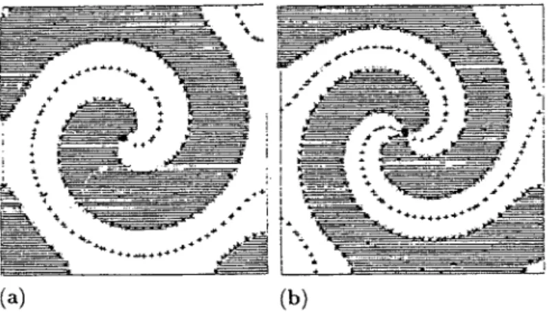
Figure 1.1. (a) Target patterns (circular waves) generated by pacemaker nuclei in the Belousov–Zhabotinskii reaction. The photographs are about 1 min apart. (b) Spiral waves, initiated by gently stirring the reagent. The spirals rotate with a period of about 2 min. (Reproduced with permission of A. T. Winfree) (c) In the slime mouldDictyostelium, the cells (amoebae) at a certain state in their group development, emit a periodic signal of the chemical, cyclic AMP, which is a chemoattractant for the cells. Certain pacemaker cells initiate target-like and spiral waves. The light and dark bands arise from the different optical properties between moving and stationary amoebae. The cells look bright when moving and dark when stationary. (Courtesy of P. C. Newell from Newell 1983)

discuss target patterns in the Field–Noyes model for the Belousov–Zhabotinskii reac-tion, which we considered in detail in Chapter 8. Their analytical methods can also be applied to other systems.

‘pace-maker’ moves round a small core ring it continuously creates a wave, which propagates out into the surrounding domain, from each point on the circle. This would produce, not target patterns, but spiral waves with the ‘core’ the limit cycle pacemaker. Once again these have been found in the Belousov–Zhabotinskii reaction; see Figure 1.1(b) and, for example, Winfree (1974), M¨uller et al. (1985) and Agladze and Krinskii (1982). See also the dramatic experimental examples in Figures 1.16 to 1.20 in Section 1.8 on spi-ral waves. Kuramoto and Koga (1981) and Agladze and Krinskii (1982), for example, demonstrate the onset of chaotic wave patterns; see Figure 1.23 below. If we consider such waves in three space dimensions the topological structure is remarkable; each part of the basic ‘two-dimensional’ spiral is itself a spiral; see, for example, Winfree (1974), Welsh et al., (1983) for photographs of actual three-dimensional waves and Winfree and Strogatz (1984) and Winfree (2000) for a discussion of the topological aspects. Much work (analytical and numerical) on spherical waves has also been done by Mimura and his colleagues; see, for example, Yagisita et al. (1998) and earlier references there.

Such target patterns and spiral waves are common in biology. Spiral waves, in ticular, are of considerable practical importance in a variety of medical situations, par-ticularly in cardiology and neurobiology. We touch on some of these aspects below. A particularly good biological example is provided by the slime mouldDictyostelium discoideum(Newell 1983) and illustrated in Figure 1.1(c); see also Figure 1.18.

Suppose we now consider the reaction diffusion situation in which the reaction kinetics has a single stable steady state but which, if perturbed enough, can exhibit a threshold behaviour, such as we discussed in Section 3.8, Volume I, and also in Section 7.5; the latter is the FitzHugh–Nagumo (FHN) model for the propagation of Hodgkin–Huxley nerve action potentials. Suppose initially the spatial domain is every-where at the stable steady state and we perturb a small region so that the perturbation locally initiates a threshold behaviour. Although eventually the perturbation will disap-pear it will undergo a large excursion in phase space before doing so. So, for a time the situation will appear to be like that described above in which there are two quite dif-ferent states which, because of the diffusion, try to initiate a travelling wavefront. The effect of a threshold capability is thus to provide a basis for a travelling pulse wave. We discuss these threshold waves in Section 1.6.

The collection of articles edited by Maini (1995) shows how ubiquitous and diverse spatiotemporal wave phenomena are in the biomedical disciplines with examples from wound healing, tumour growth, embryology, individual movement in populations, cell– cell interaction and others.

Travelling waves also exist, for certain parameter domains, in model chemotaxis mechanisms such as proposed for the slime mouldDictyostelium(cf. Section 11.4, Vol-ume I); see, for example, Keller and Segel (1971) and Keller and Odell (1975). More complex bacterial waves which leave behind a pseudosteady state spatial pattern have been described by Tyson et al. (1998, 1999) some of which will be discussed in detail in Chapter 5.

It is clear that the variety of spatial wave phenomena in multi-species reaction dif-fusion chemotaxis mechanisms is very much richer than in single species models. If we allow chaotic pacemakers, delay kinetics and so on, the spectrum of phenomena is even wider. Although there have been many studies, only a few of which we have just mentioned, many practical wave problems have still to be studied, and will, no doubt, generate dramatic and new spatiotemporal phenomena of relevance. It is clear that here we can only consider a few which we shall now study in more detail. Later in Chapter 13 we shall see another case study involving rabies when we discuss the spatial spread of epidemics.

1.2 Waves of Pursuit and Evasion in Predator–Prey Systems

If predators and their prey are spatially distributed it is obvious that there will be tem-poral spatial variations in the populations as the predators move to catch the prey and the prey move to evade the predators. Travelling bands have been observed in oceanic plankton, a small marine organism (Wyatt 1973), animal migration, fungi and vegeta-tion (for example, Lefever and Lejeune, 1997 and Lejeune and Tlidi, 1999) to menvegeta-tion only a few. They are also fairly common, for example, in the movement of primitive organisms invading a source of nutrient. We discuss in some detail in Chapter 5 some of the models and the complex spatial wave and spatial phenomena exhibited by specific bacteria in response to chemotactic cues. In this section we consider, mainly for illustra-tion of the analytical technique, a simple predator–prey system with diffusion and show how travelling wavefront solutions occur. The specific model we study is a modified Lotka–Volterra system (see Section 3.1, Volume I) with logistic growth of the prey and with both predator and prey dispersing by diffusion. Dunbar (1983, 1984) discussed this model in detail. The model mechanism we consider is

∂U

∂t = AU

1−U K

−BU V+D1∇2U,

∂V

∂t =CU V −DV+D2∇

2_V,

(1.2)

whereUis the prey,V is the predator,A,B,C,DandK, the prey carrying capacity, are positive constants andD1andD2are the diffusion coefficients. We nondimensionalise

u=U K, v=

B V A , t

∗_{= At, x}∗_=x A

D2

1/2

,

D∗= D1 D2

, a= C K

A , b=

D C K.

We consider only the one-dimensional problem, so (1.2) become, on dropping the as-terisks for notational simplicity,

∂u

∂t =u(1−u−v)+D

∂2u

∂x2,

∂v

∂t =av(u−b)+

∂2v ∂x2,

(1.3)

and, of course, we are only interested in non-negative solutions.

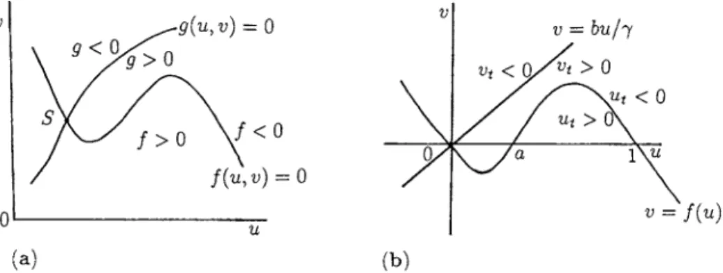
The analysis of the spatially independent system is a direct application of the pro-cedure in Chapter 3, Volume I; it is simply a phase plane analysis. There are three steady states (i)(0,0); (ii)(1,0), that is, no predator and the prey at its carrying capacity; and (iii)(b,1−b), that is, coexistence of both species ifb< 1, which henceforth we as-sume to be the case. It is left as a revision exercise to show that both(0,0)and(1,0)

are unstable and(b,1−b)is a stable node if 4a ≤ b/(1−b), and a stable spiral if 4a>b/(1−b). In fact in the positive(u, v)quadrant it is a globally stable steady state since (1.3), with∂/∂x≡0, has a Lyapunov function given by

L(u, v)₌au−b−blnu b

+

v₋1+b−(1−b)ln

_v

1−b

.

That is,L(b,1−b)₌0,L(u, v)is positive for all other(u, v)in the positive quadrant andd L/dt <0 (see, for example, Jordan and Smith 1999 for a readable exposition of Lyapunov functions and their use). Recall, from Section 3.1, Volume I that in the sim-plest Lotka–Volterra system, namely, (1.2) without the prey saturation term, the nonzero coexistence steady state was only neutrally stable and so was of no use practically. The modified system (1.2) is more realistic.

Let us now look for constant shape travelling wavefront solutions of (1.3) by setting u(x,t)₌U(z), v(x,t)₌V(z), z=x+ct, (1.4) in the usual way (see Chapter 13, Volume I) wherecis the positive wavespeed which has to be determined. If solutions of the type (1.4) exist they represent travelling waves moving to the left in thex-plane. Substitution of these forms into (1.3) gives the ordinary differential equation system

cU′=U(1−U−V)₊DU′′,

cV′₌aV(U₋b)₊V′′, (1.5)

The analysis of (1.5) involves the study of a four-dimensional phase space. Here we consider a simpler case, namely, that in which the diffusion,D1, of the prey is very

much smaller than that of the predator, namely D2, and so to a first approximation

we take D(₌ D1/D2) = 0. This would be the equivalent of thinking of a plankton–

herbivore system in which only the herbivores were capable of moving. We might rea-sonably expect the qualitative behaviour of the solutions of the system withD =0 to be more or less similar to those withD=0 and this is indeed the case (Dunbar 1984). With D = 0 in (1.5) we write the system as a set of first-order ordinary equations, namely,

U′= U(1−U−V)

c , V

′_{=W, W}′_{=cW−aV(U−b). (1.6)}

In the(U,V,W)phase space there are two unstable steady states(0,0,0)and(1,0,0), and one stable one(b,1−b,0); we are, as noted above, only interested in the case b < 1. From the experience gained from the analysis of Fisher–Kolmogoroff equa-tion, discussed in detail in Section 13.2, Volume I, there is thus the possibility of a travelling wave solution from(1,0,0)to (b,1−b,0)and from (0,0,0)to(b,1− b,0). So we should look for solutions(U(z),V(z))of (1.6) with the boundary condi-tions

U(_−∞)₌1, V(_−∞)₌0, U(_∞)₌b, V(_∞)₌1−b (1.7) and

U(_−∞)₌0, V(_−∞)₌0, U(_∞)₌b, V(_∞)₌1₋b. (1.8) We consider here only the boundary value problem (1.6) with (1.7). First linearise the system about the singular point(1,0,0), that is, the steady stateu = 1,v ₌ 0, and determine the eigenvaluesλin the usual way as described in detail in Chapter 3, Volume I. They are given by the roots of

−λ₋1

c −

1

c 0

0 −λ 1

0 −a(1−b) c−λ

=0,

namely,

λ1= −

1

c, λ2, λ3= 1 2{c± [c

2

−4a(1−b)_]1/2_}. (1.9) Thus there is an unstable manifold defined by the eigenvectors associated with the eigen-valuesλ2andλ3which are positive for allc > 0. Further,(1,0,0)is unstable in an

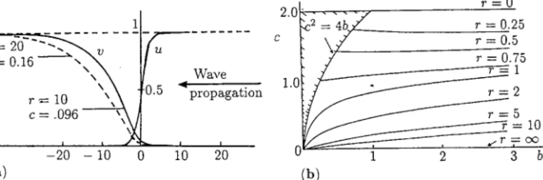
oscillatory manner ifc2<4a(1−b). So, the only possibility for a travelling wavefront solution to exist with non-negativeUandV is if

Withcsatisfying this condition, a realistic solution, with a lower bound on the wave speed, may exist which tends tou ₌1 andv₌0 asz _{→ −∞}. This is reminiscent of the travelling wavefront solutions described in Chapter 13, Volume I.

The solutions here, however, can be qualitatively different from those in Chapter 13, Volume I, as we see by considering the approach of(U,V)to the steady state(b,1₋b). Linearising (1.6) about the singular point(b,1−b,0)the eigenvaluesλare given by

−λ₋b

c −

b

c 0

0 −λ 1

−a(1−b) 0 c−λ

=0

and so are the roots of the cubic characteristic polynomial

p(λ)_≡λ3₋λ2

c−b c

−λb−ab(1−b)

c =0. (1.11)

To see how the solutions of this polynomial behave as the parameters vary we consider the plot of p(λ)for realλand see where it crossesp(λ)₌0. Differentiatingp(λ), the local maximum and minimum are at

λM, λm =

1 3





c−b c

±

c−b c

2

+3b

1/2 

and are independent ofa. Fora=0 the roots of (1.11) are

λ₌0, λ1, λ2=

1 2





c−b c

±

c−b c

2

+4b

1/2 

as illustrated in Figure 1.2. We can now see how the roots vary witha. From (1.11), asaincreases from zero the effect is simply to subtractab(1₋b)/ceverywhere from

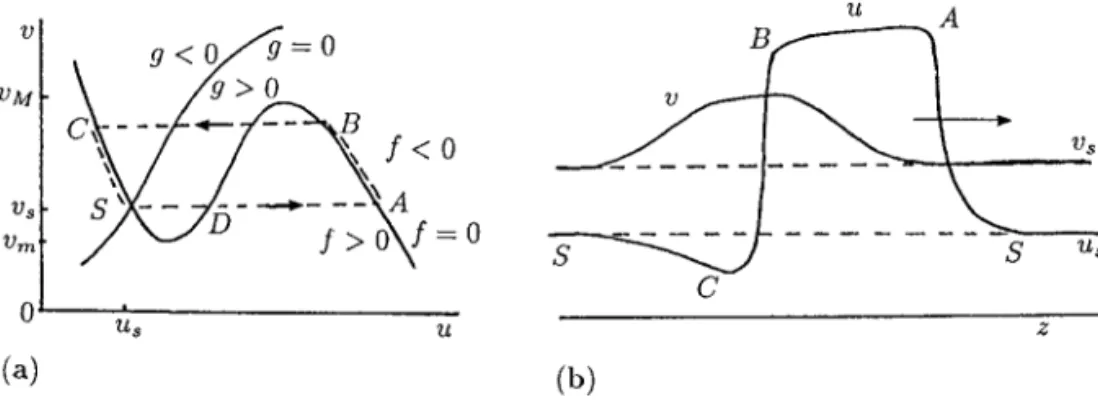
Figure 1.3. Typical examples of the two types of waves of pursuit given by wavefront solutions of the preda-tor(v)–prey(u)system (1.3) with negligible dispersal of the prey. The waves move to the left with speedc. (a) Oscillatory approach to the steady state(b,1₋b), whena>a∗. (b) Monotonic approach of(u, v)to (b,1₋b)whena_≤a∗.

the p(λ_;a₌0)curve. Since the local extrema are independent ofa, we then have the situation illustrated in the figure. For 0 < a < a∗there are 2 negative roots and one positive one. Fora ₌ a∗ the negative roots are equal while fora > a∗ the negative roots become complex with negative real parts. This latter result is certainly the case for a just greater than a∗ by continuity arguments. The determination of a∗ can be carried out analytically. The same conclusions can be derived using the Routh–Hurwitz conditions (see Appendix B, Volume I) but here if we use them it is intuitively less clear. The existence of a criticala∗ means that, fora > a∗, the wavefront solutions

(U,V)of (1.6) with boundary conditions (1.7) approach the steady state(b,1−b)in anoscillatorymanner while fora <a∗they are monotonic. Figure 1.3 illustrates the two types of solution behaviour.

The full predator–prey system (1.3), in which both the predator and prey diffuse, also gives rise to travelling wavefront solutions which can display oscillatory behaviour (Dunbar 1983, 1984). The proof of existence of these waves involves a careful analysis of the phase plane system to show that there is a trajectory, lying in the positive quad-rant, which joins the relevant singular points. These waves are sometimes described as ‘waves of pursuit and evasion’ even though there is little evidence of prey evasion in the solutions in Figure 1.3, since other than quietly reproducing, the prey simply wait to be consumed.

Convective Predator–Prey Pursuit and Evasion Models

A totally different kind of ‘pursuit and evasion’ predator–prey system is one in which the prey try to evade the predators and the predators try to catch the prey only if they interact. This results in a basically different kind of spatial interaction. Here, by way of illustration, we briefly describe one possible model, in its one-dimensional form. Let us suppose that the prey (u) and predator (v) can move with speedsc1andc2, respectively,

Figure 1.4. (a) The prey and predator populations are spatially separate and each satisfies its own dynamics: they do not interact and simply move at their own undisturbed speedc1andc2. Each population grows until

it is at the steady state(us, vs)determined by its individual dynamics. Note that there is no dispersion so the

spatial width of the ‘waves’wuandwvremain fixed. (b) When the two populations overlap, the prey put on an extra burst of speedh1vx,h1>0 to try and get away from the predators while the predators put on an

extra spurt of speed, namely,−h2ux,h2>0, to pursue them: the motivation for these terms is discussed in

the text.

Figure 1.4 and consider first Figure 1.4(a). Here the populations do not interact and, since there is no diffusive spatial dispersal, the population at any given spatial position simply grows or decays until the whole region is at that population’s steady state. The dynamic situation is then as in Figure 1.4(a) with both populations simply moving at their undisturbed speedsc1andc2and without spatial dispersion, so the width of the

bands remains fixed asuandvtend to their steady states. Now suppose that when the predators overtake the prey, the prey try to evade the predators by moving away from them with an extra burst of speed proportional to the predator gradient. In other words, if the overlap is as in Figure 1.4(b), the prey try to move away from the increasing number of predators. By the same token the predators try to move further into the prey and so move in the direction of increasing prey. At a basic, but nontrivial, level we can model this situation by writing the conservation equations (see Chapter 11, Volume I) to include convective effects as

ut− [(c1+h1vx)u]x = f(u, v), (1.12)

vt − [(c2−h2ux)v]x =g(v,u), (1.13)

where f andgrepresent the population dynamics andh1andh2are the positive

sides of the equations must be in divergence form. We now motivate the various terms in the equations.

The interaction terms f andgare whatever predator–prey situation we are con-sidering. Typically f(u,0)represents the prey dynamics where the population simply grows or decays to a nonzero steady state. The effect of the predators is to reduce the size of the prey’s steady state, so f(u,0) > f(u, v >0). By the same token the steady state generated byg(v,u=0)is larger than that produced byg(v,0).

To see what is going on physically with the convective terms, suppose, in (1.12), h1=0. Then

ut−c1ux = f(u, v),

which simply represents the prey dynamics in a travelling frame moving with speedc1.

We see this if we usez = x+c1t andt as the independent variables in which case

the equation simply becomesut = f(u, v). If c2 = c1, the predator equation, with

h2=0, becomesvt =g(v,u). Thus we have travelling waves of changing populations

until they have reached their steady states as in Figure 1.4(a), after which they become travelling (top hat) waves of constant shape.

Consider now the more complex case whereh1andh2are positive andc1 = c2.

Referring to the overlap region in Figure 1.4(b), the effect in (1.12) of theh1vx term,

positive becausevx >0, is to increase locally the speed of the wave of the prey to the

left. The effect of−h2ux, positive becauseux <0, is to increase the local convection

of the predator. The intricate nature of interaction depends on the form of the solutions, specificallyux andvx, the relative size of the parametersc1, c2,h1 andh2 and the

interaction dynamics. Because the equations are nonlinear through the convection terms (as well as the dynamics) the possibility exists of shock solutions in whichu andv

undergo discontinuous jumps; see, for example, Murray (1968, 1970, 1973) and, for a reaction diffusion example, Section 13.5 in Chapter 13 (Volume 1).

Before leaving this topic it is interesting to write the model system (1.12), (1.13) in a different form. Carrying out the differentiation of the left-hand sides, the equation system becomes

ut − [(c1+h1vx)]ux = f(u, v)+h1uvx x,

vt − [(c2−h2ux)]vx =g(v,u)−h2vux x.

(1.14)

In this form we see that theh1 andh2 terms on the right-hand sides representcross

diffusion, one positive and the other negative. Cross diffusion, which, of course, is only of relevance in multi-species models was defined in Section 11.2, Volume I: it occurs when the diffusion matrix is not strictly diagonal. It is a diffusion-type term in the equation for one species which involves another species. For example, in theu-equation, h1uvx x is like a diffusion term inv, with ‘diffusion’ coefficienth1u. Typically a cross

diffusion would be a term∂(Dvx)/∂xin theu-equation. The above is an example where

cross diffusion arises in a practical modelling problem—it is not common.

Murray and Cohen (1983), who studied the system withh1andh2nonzero. Hasimoto

(1974) obtained analytical solutions to the system (1.12) and (1.13), whereh1=h2=0

and with the special forms f(u, v) ₌l1uv,g(u, v) =l2uv, wherel1andl2are

con-stants. He showed how blow-up can occur in certain circumstances. Interesting new solution behaviour is likely for general systems of the type (1.12)–(1.14).

Two-dimensional problems involving convective pursuit and evasion are of ecolog-ical significance and are particularly challenging; they have not been investigated. For example, in the first edition of this book, it was hypothesized that it would be very inter-esting to try and model a predator–prey situation in which species territory is specifically involved. With the wolf–moose predator–prey situation in Canada we suggested that it should be possible to build into a model the effect of wolf territory boundaries to see if the territorial ‘no man’s land’ provides a partial safe haven for the prey. The intuitive reasoning for this speculation is that there is less tendency for the wolves to stray into the neighbouring territory. There seems to be some evidence that moose do travel along wolf territory boundaries. A study along these lines has been done and will be discussed in detail in Chapter 14.

A related class of wave phenomena occurs when convection is coupled with ki-netics, such as occurs in biochemical ion exchange in fixed columns. The case of a single-reaction kinetics equation coupled to the convection process, was investigated in detail by Goldstein and Murray (1959). Interesting shock wave solutions evolve from smooth initial data. The mathematical techniques developed there are of direct relevance to the above problems. When several ion exchanges are occurring at the same time in this convective situation we then have chromatography, a powerful analytical technique in biochemistry.

1.3 Competition Model for the Spatial Spread

of the Grey Squirrel in Britain

Introduction and Some Facts

About the beginning of the 20th century North American grey squirrels (Sciurus caro-linensis) were released from various sites in Britain, the most important of which was in the southeast. Since then the grey squirrel has successfully spread through much of Britain as far north as the Scottish Lowlands and at the same time the indigenous red squirrelSciurus vulgarishas disappeared from these localities.

Lloyd (1983) noted that the influx of the grey squirrel into areas previously occu-pied by the red squirrel usually coincided with a decline and subsequent disappearance of the red squirrel after only a few years of overlap in distribution.

Prior to the introduction of the grey, the red squirrel had evolved without any inter-specific competition and so selection favoured modest levels of reproduction with low numerical wastage. The grey squirrel, on the other hand, evolved within the context of strong interspecific competition with the American red squirrel and fox squirrel and so selection favoured overbreeding. Both red and grey squirrels can breed twice a year but the smaller red squirrels rarely have more than two or three offspring per litter, whereas grey squirrels frequently have litters of four or five (Barkalow 1967).

In North America the red and grey squirrels occupy separate niches that rarely overlap: the grey favour mixed hardwood forests while the red favour northern conifer forests. On the other hand, in Britain the native red squirrel must have evolved, in the absence of the grey squirrel, in such a way that it adapted to live in hardwood forests as well as coniferous forests. Work by Holm (1987) also tends to support the hypothesis that grey squirrels may be at a competitive advantage in deciduous woodland areas where the native red squirrel has mostly been replaced by the grey. Also the North American grey squirrel is a large robust squirrel, with roughly twice the body weight of the red squirrel. In separate habitats the two squirrel species show similar social organisation, feeding and ranging ecology but within the same habitat we would expect even greater similarity in their exploitation of resources, and so it seems inevitable that two species of such close similarity could not coexist in sharing the same resources.

In summary it seems reasonable to assume that an interaction between the two species, probably largely through indirect competition for resources, but also with some direct interaction, for example, chasing, has acted in favour of the grey squirrel to drive off the red squirrel mostly from deciduous forests in Britain. Okubo et al. (1989) investi-gated this displacement of the red squirrel by the grey squirrel and, based on the above, proposed and studied a competiton model. It is their work we follow in this section. They also used the model to simulate the random introduction of grey squirrels into red squirrel areas to show how colonisation might spread. They compared the results of the modelling with the available data.

Competition Model System

Denote by S1(X,T)and S2(X,T)the population densities at positionXand time T

of grey and red squirrels respectively. Assuming that they compete for the same food resources, a possible model is the modified competition Lotka–Volterra system with diffusion, (cf. Chapter 5, Volume I), namely,

∂S1

∂T =D1∇

2

S1+a1S1(1−b1S1−c1S2),

∂S2

∂T =D2∇

2_S

2+a2S2(1−b2S2−c2S1),

(1.15)

where, fori=1,2,ai are net birth rates, 1/biare carrying capacities,ciare competition

coefficients andDi are diffusion coefficients, all non-negative. The interaction

(kinet-ics) terms simply represent logistic growth with competition. For the reasons discussed above we assume that the greys outcompete the reds so

We now want to investigate the possibility of travelling waves of invasion of grey squirrels which drive out the reds. We first nondimensionalise the model system by setting

θi =biSi,i=1,2,t =a1T,x=(a1/D1)1/2X,

γ1=c1/b2, γ2=c2/b1, κ=D2/D1, α=a1/a2

(1.17)

and (1.15) becomes

∂θ1

∂t = ∇

2_θ

1+θ1(1−θ1−γ1θ2),

∂θ2

∂t =κ∇

2_θ

1+αθ2(1−θ2−γ2θ1).

(1.18)

Because of (1.16),

γ1<1, γ2>1. (1.19)

In the absence of diffusion we analysed this specific competition model system (1.18) in detail in Chapter 5, Volume I. It has three homogeneous steady states which, in the absence of diffusion, by a standard phase plane analysis, are(0,0)an unstable node,(1,0)a stable node and(0,1)a saddle point. So, with the inclusion of diffusion, by the now usual procedure, there is the possibility of a solution trajectory from(0,1)

to (1,0)and a travelling wave joining these critical points. This corresponds to the ecological situation where the grey squirrels (θ1) outcompete the reds (θ2) to extinction:

it comes into the category of competitive exclusion (cf. Chapter 5, Volume I).

In one space dimensionx ₌ xwe look for travelling wave solutions to (1.18) of the form

θi =θi(z),i=1,2, z=x−ct,c>0, (1.20)

wherecis the wavespeed.θ1(z)andθ2(z)represent wave solutions of constant shape

travelling with velocitycin the positivex-direction. With this, equations (1.18) become d2θ1

dz2 +c

dθ1

dz +θ1(1−θ1−γ1θ2)=0,

κd

2_θ 2

dz2 +c

dθ2

dz +αθ2(1−θ2−γ2θ1)=0,

(1.21)

subject to the boundary conditions

θ1=1, θ2=0, atz= −∞, θ1=0, θ2=1, atz= ∞. (1.22)

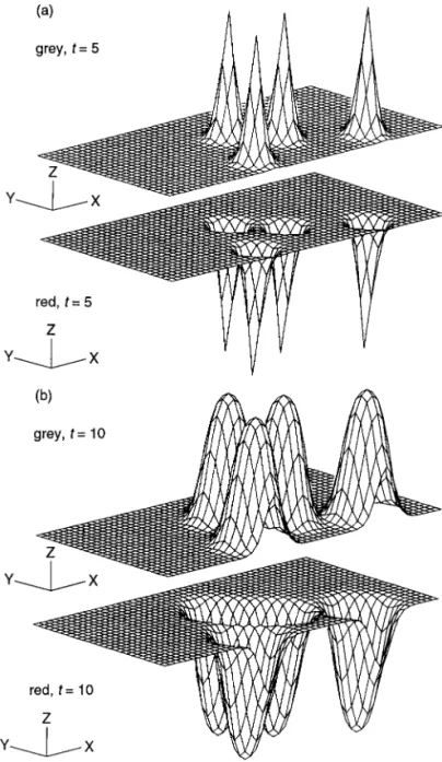
That is, asymptotically the grey (θ1) squirrels drive out the red(θ2)squirrels as the wave