Article
Printed in Brazil - ©2015 Sociedade Brasileira de Química0103 - 5053 $6.00+0.00A
*e-mail: [email protected]
Mapping Ethanol Production Sources in Brazil Through Stable Isotopes
Gilson C. Silva,a Marcelo Z. Moreira,b Arthur L. Scofield,a José M. O. Godoy,a,c Lilian F. Almeidaa and Angela L. R. Wagener*,a
aLaboratório de Estudos Marinhos e Ambientais (LABMAM), Departamento de Química,
Pontifícia Universidade Católica do Rio de Janeiro, 22451-900 Rio de Janeiro-RJ, Brazil
bLaboratório de Ecologia Isotópica, Centro de Energia Nuclear na Agricultura (CENA),
Universidade de São Paulo, 13400-970 Piracicaba-SP, Brazil
cLaboratório de Caracterização de Águas (LABAGUAS), Departamento de Química,
Pontifícia Universidade Católica do Rio de Janeiro, 22451-900 Rio de Janeiro-RJ, Brazil
Ethanol is a biofuel produced in Brazil through fermentation of sugarcane, requiring vast plantation areas and water availability. The present work aimed at testing isotopic markers as tools for ethanol source appointment or certification of origin. For this, oxygen and hydrogen isotopic patterns were determined in plant-water, soil-water, rainwater, and water from reservoirs and some rivers in four sugarcane crop areas. The isotopic fingerprint of carbon and hydrogen in ethanol produced in the respective mills was also determined. Samples were collected in 2011 and 2012 in crop areas of the state of Amazonas (North), Mato Grosso (Center-West), São Paulo (Southeast) and Rio Grande do Sul (South). The substantial and complex influence of the hydrological cycle on the ethanol δD and the small δ13C variations constrain the use of isotopes for the intended objectives.
Keywords: continuous flow isotope ratio mass spectrometry (CF-IRMS), isotope ratio infrared spectroscopy (IRIS), ethanol, water, isotopic ratios
Introduction
Ethanol is an important biofuel in the scenario of renewable and sustainable sources of energy. In Brazil it is produced via fermentation of sugarcane, a plant of the botanical group C4, (family Gramineae and genus
Saccharum), which has a high economic importance since it also yields sugar. Native to tropical climates, this plant grows under different and even adverse environmental conditions due to the development of several improved varieties as to give the best response and allow extended harvest over most part of the year.1 The typical sugarcane
biomass structure is composed of water, fiber and sugar.2
Sugarcane crops require large amounts of water, which represents 70% of its weight, mostly absorbed through the roots.3 Soil-water is closely connected to the plant-water and
also to rainwater. Rainwater infiltrates into soil subsurface where it is retained to rebuild the moisture and recharge the phreatic. Ethanol is formed during fermentation of sugars, and in this process both sugar and water medium
contribute as sources of hydrogen,4,5 while plant-water and
sugar are the sources of oxygen.6 The hydrogen atoms in the
ethanol methylene group derive from water present in the fermentative medium, composed basically of plant-water, so that the differentiation of ethanol sources involves the understanding of water cycle and its interactions in the ecosystem. In terms of carbon isotope ratios, ethanol should reflect the isotopic composition of original sugar since fermentation is not a fractionating reaction.7
18O/16O and 2H/1H of water are important tracers
in hydrogeological studies, since phase changes, like evaporation and condensation (precipitation), determines the enrichment or depletion of the heavier isotope in a water reservoir. Although gradients in the isotopic composition of soil-water may arise from differences in seasonal moisture inputs, evaporation in the uppermost surface layer as well as from differences between bulk soil moisture and groundwater, there is no isotopic fractionation during water uptake by roots and transportation to leaves.8-10 The isotopic
composition of ethanol has been used for: differentiation of botanical and geographical origins;4,11,12 evaluation of
isotopic fingerprinting in contaminated sites;13 assessment
of ethanol sources in the atmosphere14 and investigation
of alcoholic beverages adulteration.15,16 Despite the
widespread ethanol production in Brazil, in sites of diverse climatic properties, no evaluation has been reported of regional conditions on the isotopic fingerprinting of ethanol.
Brazil is one of the most important ethanol producers17,18
with the mean annual production of 21.3 billion m3 (for the
2003-2012 period)19 carried out in at least 378 registered
active sugarcane mills20,21 and has the potential to be the
most important exporter of this commodity. Because the expansion of agricultural frontier may represent a threat to forested ecosystems and protected areas,22 it is pertinent to
identify tools that can be used to detect the provenance of ethanol and to certify its origin.
The specific objectives of this work were: (i) to assess oxygen and hydrogen isotopic patterns in plant-water, soil-water, rainwater, and water from reservoirs and rivers associated to four Brazilian sugarcane crop areas; (ii) to determine carbon and hydrogen isotopic fingerprint of ethanol produced in the same areas as to evaluate regional isotopic patterns, seasonal variations, and the influence of hydrological cycle/climatic conditions on ethanol isotopic ratios. Relationship between carbon isotope ratio of ethanol and sugarcane biomass was also investigated. The general aim of the work was testing tools for identification of ethanol geographical origin and source appointment.
Experimental
Study area
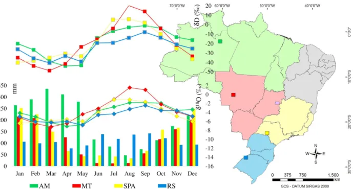
All samples in this study were collected in sugarcane mills and nearby not irrigated crops distributed in four different locations covering distinct geographical regions of Brazil (Figure 1): Amazonas (AM, North), Mato Grosso (MT, Center-West), São Paulo (SPA, Southeast) and Rio Grande do Sul (RS, South). Reference spots for rainwater isotopic pattern and precipitation amount were selected among the nearest stations of the Global Network for Isotopes in Precipitation (GNIP) database23 and the National
Institute of Meteorology (INMET) database,24 respectively.
Sampling campaigns in AM were performed in Agropecuária Jayoro mill (1° 59’ 17.85” S 60° 8’ 27.39” W, altitude 144 m), in Presidente Figueiredo municipality. The average annual temperature in this location is 25 °C and the annual average rainfall of 2,500 mm.25,26 Presidente
Figueiredo lies on the basin of Uatumã River, in the limits of the hydrographic sub-regions of Negro and Trombetas rivers, which belong to the hydrographic basin of the Amazon River.27 Soil type is dystrophic yellow latosol.26
Sampling campaigns in MT were performed in Coprodia mill (13° 47’ 17.33” S 57° 50’ 31.31” W, altitude 528 m), in Campo Novo do Parecis municipality. Average temperature ranges between 24 and 40 °C in this location, where two climatic types predominate: Equatorial hot and humid, and tropical hot and sub-humid. The first climate
type includes three dry months, from June to August, and intense rainfall from January to March dominated by the Equatorial continental air mass; the second climate type includes four dry months, from June to September, and a rainfall period from December to February, dominated by continental tropical air mass.27 The mean annual
precipitation is 1,796 mm.28 Water provision for this
mill derives from an affluent of Do Sangue River in the Juruena-Arinos River basin, located in the Tapajós River hydrographic sub-region, which, in turn, fits in the Amazon River hydrographic region.27,29 Three soil types are found
in this location: quartz sand, red and dark red latosols.27
Sampling campaigns in SPA were performed in Pau D’Alho mill (22° 46’ 4” S 50° 6’ 43” W, altitude 458 m), located in Ibirarema municipality. The climate is tropical with annual isothermal temperature in the range of 20 to 22 °C and mean annual precipitation of 1,511 mm; the rainy season occurs from November to February. In general, weather conditions in this hydrographic region depends on a series of factors, such as tropical Atlantic mass control, invasion of cold fronts, incursions of the continental tropical air mass associated with Chaco Low (typical low pressure system), presence of south Atlantic convergence zone (SACZ) and disturbances caused by the relief. This place lies in the hydrographic region of Paraná River, in Paranapanema sub-basin. Structured purple ground soil predominates in this location.30,31
Sampling campaigns in RS were performed in Coopercana mill (27° 54’ 18.35” S 55° 9’ 37.92” W, altitude 125 m), located in Porto Xavier municipality, near the Argentinean border, and only 2 km away from Uruguay River. In this location climate is temperate, average annual temperatures ranges from 16 to 20 °C increasing from May to September; intra-annual rainfall distribution is regular with an annual average of 1,784 mm. Atmospheric circulation is governed by tropical and polar air mass systems, with tropical Atlantic (Ta) and polar Atlantic (Pa) predominating alternately in all seasons.31,32 This location
lies in the so-called medium Uruguay area, in Ijuí River hydrographic sub-region which is part of the Uruguay River hydrographic region.32 Dystrophic red latosol soil
predominates in this location.
GNIP reference stations for rainwater isotopic ratios located in Manaus (AMGNIP), Cuiabá (MTGNIP) and Porto Alegre (RSGNIP) has data survey for the period from
1965 to 1987. Because results for São Paulo State are scarce, existing GNIP data for the period 1996 to 199823
obtained in Santa Maria da Serra, Campinas, Bragança and Piracicaba stations (SPAGNIP) were used. Historical data
for mean monthly and annual accumulated precipitation were available for the INMET stations located in Manaus
(AMINMET), Cuiabá (MTINMET), Porto Alegre (MTINMET),
Santa Rita and Campinas (SPAINMET) in the period from 1961 to 1990.24
Sampling
Sampling campaigns carried out in August and November, 2011, included ethanol, sugarcane and rainwater samples (pilot study), and those in July and October-November, 2012 included ethanol, sugarcane, rainwater, surface waters and soil samples. Additional surface and groundwater were sampled in MT on September, 2014 for confirmation of groundwater isotopic profile. Ethanol and water samples were stored refrigerated at −4 °C while plant
and soil samples were kept frozen at −18 °C.
Ethanol samples were collected from the reservoirs of the respective mill in clear glass flasks fitted with screw caps faced with polytetrafluoroethylene (PTFE), and protected from light with aluminum foil.
Rainwater samples were collected during individual rain events, a couple of days before sampling of the other matrices, using glass bottles fitted with funnel or large aluminum recipients, then transferred to clear glass flasks fitted with screw caps faced with PTFE. The only exception was the sample collected in MT, which integrated all precipitations throughout October, 2012. Surface and groundwater were collected from open water systems and artesian wells, respectively, directly into clear glass flasks fitted with screw caps faced with PTFE.
Plant samples were collected from the crop, in the neighborhood of the mills, by cutting a transverse section at half height of the plant. In 2011, sampling involved the collection of a single plant in each spot, which was involved in polyethylene film and stored in a polyethylene flask sealed with PTFE film, while in 2012 plants were collected from every 10 m along the perimeter of a square of 20 × 20 m, plus one in the center, amounting to 9 sub samples that were gathered as a final composite sample and kept in an aluminum flask sealed with PTFE film.
Soil samples were collected only in 2012, from 0-5 cm and 20-25 cm depths, near the plant root system, in the center of the referred square described for plant samples, and kept in an aluminum flask sealed with PTFE film.
Analysis
samples were filtered through 0.45 µm filters and injected 6 times, discharging the 3 first results to avoid memory effect. Plant- and soil-water were previously extracted by vacuum distillation in a specially designed apparatus that allowed the processing of six-sample batches twice a day. Water samples extracted from plants were also treated over activated charcoal for several days to eliminate any co-extracted organic contaminant. Analytical precisions, expressed as standard deviations, were better than ± 0.60‰ for δ18O and ± 2.80‰ for δD for water and soil-water
results, while for plant-water they were better than ± 0.74‰ for δ18O and ± 3.60‰ for δD.
An inter-laboratory comparison was performed for the plant-water samples using an analyzer model L2130-I, based on wavelength-scanned cavity ring-down spectroscopy, fitted with a vaporizer model A0211 and a micro-combustion module (WS-CRDS; Picarro Inc., Sunnyvale, CA, USA). The procedures are detailed by Godoy et al.33 and analytical precisions were better
than ± 0.25‰ for δ18O and ± 0.60‰ for δD.
Determinations of δ13C and δD in ethanol were performed
via continuous flow isotope ratio mass spectrometer (CF-IRMS). Before analysis, all samples were dehydrated using molecular sieve UOP type 3A (Sigma-Aldrich, Fluka, St Louis, USA) according to Monsallier-Bitea et al.15 and
Jamin et al.34 The molecular sieve was previously activated at
300 °C for 4 h, added in small amounts to the vials containing samples and then kept refrigerated overnight. Dehydrated samples were diluted to 1 mmol L–1 in isooctane and either
injected in 1:100 split for carbon analyses or without dilution in splitless mode for hydrogen analyses. Pro analysis grade ethanol (VETEC, Duque de Caxias, RJ, Brazil) was used as working standard to evaluate the performance of the analytical system at every 20 injections. Analytical precisions were better than ± 0.15‰ for δ13C and ± 4.8‰ for δD.
Analytical system was composed of a CF-IRMS Deltaplus V (ThermoFinnigan, Bremen, Germany) with open split, connected in-line via Conflo 4 system to a gas chromatograph Trace GC Ultra interfaced by an Isolink combustion oven (Thermo Electron S.p.A, Milan, Italy). GC was equipped with a capillary column HP DB-624 (30 m × 0.45 mm i.d., 2.55 µm film) and the analysis conditions were as follows: injector temperature, 250 °C; split injection mode with ratio 100:1 (for carbon analysis) or splitless (for hydrogen analysis); split flow at 150 mL min–1;
carrier gas in constant flow mode, 1.5 mL min–1; oven
temperature program: 45 °C for 5 min, raising from 45 °C to 190 °C at 35 °C min–1 and 190 °C for 1 min. Injection
volumes were 2 µL. Isolink ovens were set at 1000 °C and 1400 °C for carbon and hydrogen isotope ratios, respectively.
Confirmation of isotopic ratios for the ethanol working standard as well as the determinations of δ13C in sugarcane
samples were performed in an elemental analyzer Flash EA 1112 (ThermoQuest, Milan, Italy) equipped with combustion and thermal conversion reactors and coupled to the IRMS (EA-IRMS). The combustion reactor (conversion to CO2 at 1020 °C) was prepared with quartz tube filled with chromium oxide, 50 mm; reduced copper, 110 mm; silvered cobaltous/ cobaltic oxide, 30 mm, and 1 mm quartz wool layer on top, bottom and between layers. The thermal conversion reactor (conversion into H2 at 1450 °C) was prepared with a ceramic
tube containing a glassy carbon reactor tube (270 mm), a graphite crucible, glassy carbon granulate, 100 mm; silver wool, 5 mm; glassy carbon granulate, 15 mm, quartz wool, 15 mm, and silver wool, 5 mm.
Sugarcane samples were freeze-dried and ground in an analytical mill A11 Basic (IKA Works Inc., North Carolina, USA) before analyses. Ethanol standard was introduced in the analytical system through the autosampler for solids, using adsorbents to avoid evaporation and consequent fractionation before conversion in the reactor. For δ13C analysis ethanol was previously supported over
Chromosorb W, as described by Adami et al.,11 while for δD analyses ethanol was supported over activated charcoal
previously treated by heating at 170 °C for 4 h. Activated charcoal was chosen because it does not contain hydrogen atoms and is a cheap and readily available adsorbent. No previous citation was found in the consulted literature about the application of active charcoal for isotope analysis purposes.
Stable isotope ratios are expressed in δ notation (‰)
and were calculated according to the following equation:
Rsample
– 1 × 1000 Rstandard
δ =
where Rsample and Rstandard represent the isotope ratios (13C/12C
and D/H) of samples and standard material, respectively. The reference materials used for calibration were: USGS 40, L-glutamic acid (δ13C
VPDB-LSVEC = −26.39 ± 0.04‰) and
IAEA-CH-7, polyethylene (δDVSMOW = −100.3 ± 2.0‰),
and Vienna standard mean ocean water (VSMOW). All isotopic ratios are reported relative to VSMOW and VPDB.
was confirmed by evaluation of residuals of the statistical model using Shapiro-Wilk and Kolmogorov Smirnov tests.
Results and Discussion
Sampling campaigns were carried out during the months of August and November, 2011 and July and October/ November, 2012. The 2011 campaign was a pilot study comprising only sugarcane, rainwater and ethanol samples. Obtained data revealed a complex relation between these matrices, so that new sampling campaigns were planned and carried out in 2012 including surface- and soil-water, aiming at a better understanding. Sampled sugarcane varieties were the most representative in the production of each mill. Since in Brazil there is a continuous overturn of varieties cultivated along the year, it was not possible to keep a control area or collect a specific variety along subsequent sampling campaigns.
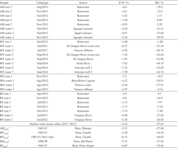
Results of δ18O and δD for rain and surface water
obtained in the present work are presented in Table 1, followed by those for plant- and soil-water in Table 2. Results of δD and δ13C for ethanol and sugarcane are
presented in Table 3.
The statistical tests with ethanol results indicated data normal distribution therefore variance analysis based on ANOVA was applied.
Interlaboratorial comparison of plant-water results
Plant-water analysis by IRIS can be biased due to the presence of residual methanol or ethanol after distillation procedure,35,36 resulting in discrepancies in δ18O and δD
values of up to 7.97‰ and 13.70‰ for water extracted from stem samples.35 This problem can be corrected by use of
a post-processing software in OA-ICOS equipments (not applied in this work), as long as the expected amount of these contaminants is known, what requires comparison of results with those from CF-IRMS or another technique to eliminate the interference. All water samples in this study were analyzed in the Los Gatos DLT-100 equipment, and to check for possible bias in the obtained results, these samples were re-analyzed in a Picarro L2130-I equipment doted of a micro-combustion module, thereby eliminating any organic interference. Isotope differences between mean results varied between 0.58 to 2.25‰ (median 0.20‰) for oxygen and 0.25 to 7.25‰ (median 2.57‰) for hydrogen. Statistical comparison of their variances (F test) and means (t-test), showed that respectively 83% and 78% of the δ18O
and δD results were not statistically different at significance levels of 0.05 to 0.02 (Tables S1 and S2 in Supplementary Information (SI) section).
Rainwater, surface and groudwater
Results for both δ18O and δD in rain and surface waters
were found in a broad range, although precipitation showed the largest variability (Table 1). As mentioned in the Study area section, hydrological patterns for these locations were estimated by comparison with historical data from GNIP stations and INMET stations (Figure 1).
Rain amount has important influence upon isotopic ratios of rainwater due to the so-called amount effect, resulting in enriched rainwater during the dry season,10,37
as shown in Figure 1, for all reference stations. In AM, the largest rain amount occurs by the beginning of the year; in MT an important drought follows in the middle of the year similarly, but attenuated, in respect to SPA; and RS has a regular distribution of rain along the entire year. In MT, virtually no rain occurs in the crop area during all the harvest period from May to October, and the influence of this climatic condition is revealed in the plant-water and soil-water isotopic ratios, as it will be discussed later. Isotopic fluctuations in the rainfall in tropical regions seem to be governed by the rain-out process in the surrounding region instead of depending on the rain-out history,38 so
that the comparison with GNIP and INMET data can be considered a good approach for isotopic amount effects in this study.
Except for MT, surface water results were close to
δ18O and δD mean values of −4.54‰ and −27.65‰ for
2011-2012 samplings (Table 1). These values are in good agreement with the weighted average of δ18O and δD for
annual rainfall in the GNIP reference stations (Table 1), which should represent groundwater isotopic fingerprint in these hydrographic basins.10,39 The differences observed for
MT samples may be attributed to the severe drought which occurs regularly from May to October in that location. Comparison of river and groundwater MT results with the weighted average for δ18O and δD in the reference
MTGNIP during the rainy season (Table 1) revealed isotopic depletion in this location resulting from the recharge period in the catchment basin. This evaluation strongly indicates that aquifers and water reservoirs observed in this work reproduce groundwater isotopic fingerprint due to phreatic recharge by rainwater. The two vinasse samples, by-products from sugarcane milling process collected from dikes in MT and SPA, seem to be highly enriched in relation to fresh surface water, probably due to evaporation.
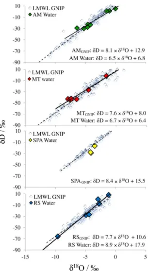
Craig40 reported a global relationship between δ18O and δD in precipitation known as the global meteoric water
line (GMWL), which can be expressed by the regression
δD = 8δ18O + 10 and provides important information
function of local temperature, altitude and distance from ocean. Reference local meteoric water lines (LMWLGNIP) were drawn using GNIP rainwater data and compared with respective LMWL obtained from water samples collected in the present work (Figure 2). In these plots, slope values below that of LMWLGNIP indicate enrichment, typical for water from reservoirs, e.g., lakes, which are more likely to evaporate, while slopes above LMWLGNIP should represent a depletion, which may have several causes, such as the altitude and continental effects.10 AM and MT showed
LMWL slopes similar to each other and both smaller than the respective LMWLGNIP station. The smaller slope in LMWL for AM samples in relation to the respective LMWLGNIP may be due to the contribution of isotopically enriched water vapor released by evapotranspiration from
the Amazon forest, while the steaper line in LMWL for RS samples must be related to the orographic complexity and latitudinal positioning41 of that site. Due to the reduced
number of samples no reliable LMWL could be drawn for SPA location.
Climatic events capable of causing alterations in the isotope ratios in this study, such as the El Niño and La Niña, were considered. These events are disruptions of the ocean-atmosphere system in the tropical Pacific characterized by unusually warm or unusually cold ocean temperatures¸ respectively, in the Equatorial Pacific, and which have important consequences for weather around the globe including changes in rain amount in Brazil, which could affect isotopic patterns of rainfall influencing results obtained in this work.42 Evaluation of oxygen and hydrogen
Table 1. Isotopic ratios for surface water and GNIP reference stations
Sample Campaign Source δ18O / ‰ δD / ‰
AM rain 1 Aug/2011 Rainwater −6.4 −29.2
AM rain 2 Nov/2011 Rainwater −4.6 −22.7
AM rain 3 Oct/2012 Rainwater −1.02 1.17
AM rain 4 Oct/2012 Rainwater −1.49 0.89
AM rain 5 Nov/2012 Rainwater −0.03 5.29
AM water 1 Oct/2012 Igarapé (stream) −4.20 −23.41
AM water 2 Oct/2012 Igapó (stream) −4.67 −27.68
AM water 3 Nov/2012 Igarapé (stream) −5.26 −29.95
MT rain 1 Oct/2012 Rainwater −1.60 −1.80
MT water 1 Jul/2012 Do Sangue River (reservoir) −6.53 −43.36
MT water 2 Jul/2012 Vinasse effluent −4.56 −26.74
MT water 3 Sep/2014 Do Sangue River (reservoir) −7.44 −42.64
MT water 4 Sep/2014 Do Sangue River −7.95 −42.96
MT water 5 Sep/2014 Verde River −7.62 −44.15
MT water 6 Sep/2014 Artesian well 1 −7.42 −43.05
MT water 7 Sep/2014 Artesian well 2 −7.39 −42.74
SPA rain 1 Nov/2011 Rainwater −3.5 −16.5
SPA water 1 Ago/2012 Bom Retiro Lagoon −4.12 −29.01
SPA water 2 Ago/2012 Process water −4.20 −27.91
SPA water 3 Ago/2012 Vinasse effluent −2.55 −13.6
RS rain 1 Ago/2011 Rainwater −2.9 0.3
RS rain 2 Nov/2011 Rainwater −9.6 −65.9
RS rain 3 Jul/2012 Rainwater −1.13 7.97
RS rain 4 Oct/2012 Rainwater −2.73 −7.52
RS rain 5 Oct/2012 Rainwater −2.74 −7.89
RS water 1 Jul/2012 Uruguay River −4.90 −27.95
RS water 2 Oct/2012 Uruguay River −4.38 −26.85
Surface water mean values (2011-2012) −4.54 −27.65
AMGNIPa 1965-87 Rain, Manaus −5.15 −27.68
MTGNIPa 1965-87 Rain, Cuiabá −5.40 −34.56
MTGNIPb 1965-87 (Nov-Apr) Rain, Cuiabá −6.15 −40.65
SPAGNIPa 1996-98 Rain, São Paulo −5.15 −27.95
RSGNIPa 1965-87 Rain, Porto Alegre −4.83 −25.84
isotopic ratios from reference GNIP stations showed that rain water becomes usually isotopicaly enriched for both elements during El Niño episodes in comparison to regular periods, while no strong tendency is observed during La Niña events (Figure S1 in the SI section). The GNIP data shows that La Niña has little or no impact on the isotopic fingerprint. The November 2011 sampling campaign carried out during such event may then be evaluated under the same conditions as those used for the other campaigns occurring in normal periods.
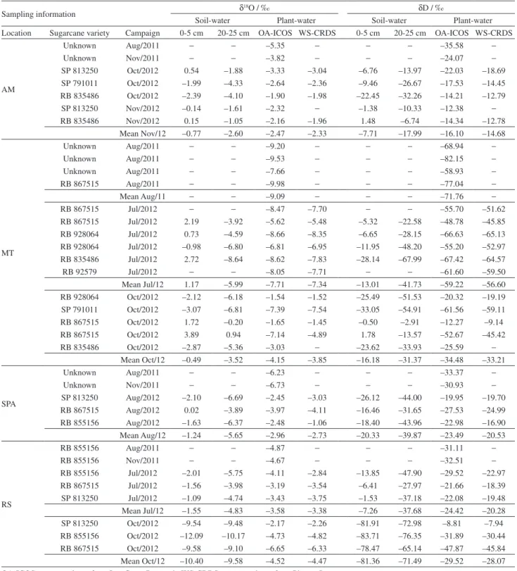
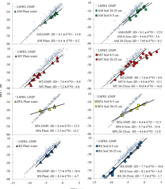
Plant-water and soil-water
In general, isotope ratios for water extracted from soil and plant samples showed considereable spread (Table 2). Plant-water was in the range of –9.98 to –1.54‰ for δ18O
and –82.15 to –8.81‰ for δD, while soil-water showed δ18O
in the range of –12.09 to 3.89‰ and for δD from –83.71 to 1.78‰, all relative to VSMOW. Despite the variability of plant-water results, the proximity with the weighted
average for rainfall (Table 1), representing the isotope fingerprinting of groundwater, reflects the connection among this compartment, soil- and plant-water, since soil water, which recharges groundwater and is absorbed by plant roots, is fed by rainwater. In general, the most depleted plant-water both in 18O and D were found in MT samples,
while RS samples showed the least variation. Having in mind the considerable natural variability of the studied system, the results point to a reasonable parity between soil-water (20-25 cm) and the respective plant-soil-water average isotopic ratios, while this does not occur for soil-water from the top layer (0-5 cm). Differences between soil- and plant-water in both cases may derive from: (i) fractionation due to evaporation and/or mixing of waters from the vadose zone with water from recent rain events; (ii) water uptake by sugarcane from deeper soil layers then better reflecting the groundwater isotopic fingerprint. Studies9,10,43 on
the isotopic fractioning of water at different soil depths (Figure 3) show kinetic isotopic effects increasing as soil moisture decreases, so that strong fractionation may be expected for samples near surface, while there is a tendency for water in vadose zone to be isotopically similar to that from the phreatic. Indeed the 0-5 cm soil-water samples gave results dramatically enriched in respect to soil samples collected at 20-25 cm depth. Despite most of sugarcane root system being found close to surface (about 63% on the top 30 cm), it can eventually reach a maximum depth of 1.5 to 2 m (Figure 3).44
Amazonas
Plant-water results for August and November, 2011 campaigns in AM (δ18O = –5.35‰, δD = –35.58‰ and
δ18O = –3.82‰, δD = –24.07‰, respectively; see Table 2)
were consistent with those from local rain samples (δ18O = –6.4‰, δD = –29.2‰ and δ18O = –4.64‰,
δD = –22.7‰; see Table 1) and also with the isotopic fingerprint of groundwater, represented by the weighted average for annual rainfall (δ18O = –5.15‰, δD = –27.68‰,
AMGNIP; see Table 1). Contrasting with these data, plant-water for October-November, 2012 campaign was more enriched (δ18O and δD mean values: –2.47‰ and
–16.10‰, respectively) with isotopic ratios between those for rainwater collected in the same period (δ18O and δD
mean values: –0.85‰ and 2.45‰, respectively, n = 3; see Table 1) and groundwater (δ18O and δD mean values:
samples collected at 20-25 cm depth, suggesting major contribution of groundwater (δ18O and δD mean values
–4.21‰ and –29.46‰, respectively, n = 2; see Table 2) and influence of rainwater (δ18O and δD mean values
–1.51‰ and –10.34‰, n = 3; see Table 2). The plot of δ18O versusδD for plant-water and soil-water (Figure 4) shows
profiles consistent with those observed for meteorical water (Figure 2) in the location, although the obtained slope is somewhat smaller than that of LMWLGNIP. Such profile supports the observations described above and indicates robust connections with the local water cycle possibly due to the high annual rainfall volume.
Table 2. Results for δ18O and δD in plant-water and soil-water
Sampling information δ
18O / ‰ δD / ‰
Soil-water Plant-water Soil-water Plant-water Location Sugarcane variety Campaign 0-5 cm 20-25 cm OA-ICOS WS-CRDS 0-5 cm 20-25 cm OA-ICOS WS-CRDS
AM
Unknown Aug/2011 − − –5.35 − − − –35.58 −
Unknown Nov/2011 − − –3.82 − − − –24.07 −
SP 813250 Oct/2012 0.54 –1.88 –3.33 –3.04 –6.76 –13.97 –22.03 –18.69 SP 791011 Oct/2012 –1.99 –4.33 –2.64 –2.36 –9.46 –26.67 –17.53 –14.45 RB 835486 Oct/2012 –2.39 –4.10 –1.90 –1.98 –22.45 –32.26 –14.21 –12.79
SP 813250 Nov/2012 –0.14 –1.61 –2.32 − –1.38 –10.33 –12.38 −
RB 835486 Nov/2012 0.15 –1.05 –2.16 –1.96 1.48 –6.74 –14.34 –12.78 Mean Nov/12 –0.77 –2.60 –2.47 –2.33 –7.71 –17.99 –16.10 –14.68
MT
Unknown Aug/2011 − − –9.20 − − − –68.94 −
Unknown Aug/2011 − − –9.53 − − − –82.15 −
Unknown Aug/2011 − − –7.66 − − − –58.93 −
RB 867515 Aug/2011 − − –9.98 − − − –77.04 −
Mean Aug/11 − − –9.09 − − − –71.76 −
RB 867515 Jul/2012 − − –8.47 –7.70 − − –55.70 –51.62
RB 867515 Jul/2012 2.19 –3.92 –5.62 –5.48 –5.32 –22.58 –48.78 –45.85 RB 928064 Jul/2012 0.73 –4.59 –8.66 –8.35 –6.65 –28.15 –66.63 –65.13 RB 928064 Jul/2012 –0.98 –6.80 –6.81 –6.95 –11.95 –48.20 –55.20 –52.97 RB 835486 Jul/2012 2.72 –8.64 –8.62 –7.83 –28.14 –67.99 –67.42 –64.57
RB 92579 Jul/2012 − − –8.05 –7.71 − − –61.60 –59.50
Mean Jul/12 1.17 –5.99 –7.71 –7.34 –13.01 –41.73 –59.22 –56.60 RB 928064 Oct/2012 –2.12 –6.18 –1.54 –1.52 –25.49 –51.53 –20.32 –19.19 SP 791011 Oct/2012 –3.07 –6.81 –7.39 –7.54 –33.05 –54.91 –61.56 –59.11 RB 867515 Oct/2012 1.72 –0.20 –1.65 –1.45 –0.50 –2.91 –12.27 –9.14 RB 867515 Oct/2012 3.89 0.94 –7.14 –4.89 1.78 –13.57 –52.67 –45.42
RB 835486 Oct/2012 –2.87 –5.36 –3.03 − –23.62 –33.93 –25.59 −
Mean Oct/12 –0.49 –3.52 –4.15 –3.85 –16.18 –31.37 –34.48 –33.21
SPA
Unknown Aug/2011 − − –6.23 − − − –33.37 −
Unknown Nov/2011 − − –6.73 − − − –30.93 −
SP 813250 Aug/2012 –2.10 –6.69 –2.45 –3.03 –26.12 –44.00 –19.95 –19.70 RB 867515 Aug/2012 0.02 –3.89 –3.97 –4.11 –16.46 –31.65 –27.53 –24.99 RB 855156 Aug/2012 –1.63 –6.37 –2.48 –1.06 –18.40 –43.96 –22.98 –16.90 Mean Aug/12 –1.24 –5.65 –2.96 –2.73 –20.33 –39.87 –23.49 –20.53
RS
RB 855156 Aug/2011 − − –4.87 − − − –31.11 −
RB 855156 Nov/2011 − − –4.67 − − − –32.51 −
Mato Grosso
Plant- and soil-water from MT were the most depleted as shown in Table 2. This site is located at 528 m high and 275 km northwest from the reference station MTGNIP
in Cuiabá (165 m height), therefore isotopically depleted rainwater should be expected in relation to Cuiabá due to altitude and continental effects.10,39,45,46 However, as the
crop is not irrigated and the sampling location undergoes severe drought during all the harvest period, the only important sources of water in August, 2011 and July, 2012 were the vadose zone and the phreatic. δ18O and δD
mean values found for plant-water (–9.09‰ and –71.76‰, respectively) in August, 2011 and in July, 2012 (–7.71‰ and –59.22‰, respectively; see Table 2 and Figure 3) differ from the predicted groundwater isotopic fingerprint based on the weighted average for annual rainfall (MTGNIPa; see
Table 1). 18O and D were actually more depleted than the
estimated groundwater based on historical MTGNIP data for
precipitation in the rain period extending from November to April (MTGNIPb; see Table 1 and Figure 1).
Although the sampling location in Campo Novo do Parecis and the GNIP station in Cuiabá pertain to different hydrographic regions,27 water isotope ratios in
the mill’s catchment point (MT water 1; see Table 1) were not significantly different from those of the estimated November-April MTGNIP groundwater. Nevertheless,
MT water 1 values may be biased due to evaporative enrichment along the course of the river47 or during the
time it resided in the large open mill’s reservoir. For further investigation on the location water and groundwater profile a complementary sampling was conducted in September, 2014. Samples were collected in four points: the mill’s reservoir (same of MT water 1), Do Sangue River, Verde River, and in two artesian wells inside the mill’s facilities. The new data were in good agreement with those from MT water 1 and confirmed the local groundwater isotopic fingerprint, the early recharge period, and the mean composition of precipitation in the catchment basin. The differences observed between these results and those from plant-water (Table 2) indicate that vadose zone may be the source of water for the sugarcane crop during 2011 and 2012 drought periods, rather than groundwater. The plot of δ18O versusδD for plant-water (Figure 4) shows
similar slope to MTGNIP, demonstrating that evaporative enrichment does not occur; the only possible conclusion is the occurrence of strongly depleted rainwater in Campo Novo do Parecis during the rainy season.
October marks the beginning of the rainy season and the end of the harvest in the mill. The integrated δ18O and
δD for precipitation throughout this month were –1.60‰ and –1.80‰, respectively, confirming the expected high enrichment caused by the amount effect, also registered in historical data for the reference station MTGNIP (δ18O
with the residual old vadose water. It is also evident an isotopic enrichment of the plant-water reaching δ18O and
δD mean values of –4.15‰ and –34.48‰, respectively. Large isotopic enrichment was observed in soil-waters collected at 0-5 cm and at 20-25 cm depth (Table 2). The enrichment in the upper layer indicates incidence of evaporative process. The plot of δ18O versus δD for
plant-water and for soil-water (Figure 4), shows profiles consistent with those observed for local meteorical water (Figure 2), except for 0-5 cm soil-water. In this case, regression slope was significantly smaller than that for LMWLGNIP, confirming a remarkable evaporative enrichment in the upper soil layer.
São Paulo
Results in SPA were atypical since only one sugarcane sample, collected on August, 2011 campaign (RB 867515, Table 2), presented results for plant-water consistent with the other matrices, like the respective soil-water (Table 2), lagoon and process waters (SPA water 1 and SPA water 2, Table 1). Additionally, the two remaining soil samples were highly depleted, with δ18O and δD mean values of
–6.53‰ and –43.98‰, respectively. The considerably reduced slopes of the linear regression for both plant and soil-water versus LMWLGNIP indicate strong isotopic enrichment in the SPA area (Figure 4). Groundwater isotopic trends in that area48 (isoscape with δ18O = –8‰
and δD = –50‰) and results of highly depleted mineral water samples (δ18O and δD mean values of –8.00‰ and
–54.54‰, respectively) collected in sites up to 150 km away from the mill32 (Águas de Santa Bárbara and Bauru
cities) fitted well when interpolated in the regression line of LMWLGNIP (plot not shown). These literature results support the predicted isotopic fingerprint for that area but, also highlight the extraordinary isotopic shifts obtained for SPA samples. Further investigation must be carried out to better understand the processes leading to such shifts.
Rio Grande do Sul
In RS, plant-water presented the most constant results, with δ18O and δD mean values of –4.22‰ and –28.18‰,
respectively. These values are consistent with those for the Uruguay River water obtained in July and November, 2012 (RS water 1 and RS water 2; see Table 1), with the weighted average for the annual rainfall (RSGNIPa, Table 1), and also
with groundwater isotopic trends in the area49 (isoscape
with δ18O –4.7‰ and δD –29‰). These plant-water results
do not concur with those for sampled precipitation, as the four rainwater samples collected presented isotopic shifts
in a broad range of δ18O ( –1.13 to –9.6‰) and δD (–0.3
to –65‰) (Table 1). Soil-water was significantly more depleted than plant-water (Table 2). In October, 2012, soil-water 18O and D were strongly depleted in respect to
July, suggesting that an important recent rain event led to shifting δ18O and δD mean values to –9.99‰ (± 1.08‰)
and –76.43‰ (± 6.73‰), respectively, in both sampled depths. The incidence of recent rain event and its effects on the isotopic results for October, 2012 soil-water is similar to the observed in November, 2011 for sample RS Rain 2 (Table 1), and also seem to have impact on the plant-water isotopic ratios. The spread of plant-water δ18O and δD
values suggest water uptake from mixed sources such as the highly isotopicaly depleted rain event, the sampled rainwater and groundwater. The δ18O versus δD linear
regressions for both plant-water and soil-water (Figure 4) were compared to the LMWLGNIP showing similar slopes,
reinforcing these conclusions.
Ethanol and sugarcane
IRMS and nuclear magnetic resonance (NMR) are the two main analytical techniques used for determination of stable isotopes in ethanol50 to assess adulteration in
beverages. In this work, the 21 samples of hydrated, anhydrous and neutral ethanol collected in the four studied mills in 2011 and 2012 harvests were analysed for δD and
δ13C using CF-IRMS. Results were in the range –216.1 to
–186.9‰ for δD and –13.24 to –12.04‰ δ13C (Table 3).
Comparison of δD for ethanol samples with those for water extracted from the sugarcane crops used in the respective mill (Tables 2, 3 and Figure 5) revealed similar general trends, showing that independently of the ethanol specification (hydrated, anhydrous or neutral ethanol),
δD is strongly influenced by the isotopic ratio from the plant-water, and consequently by the isotopic fluctuations inherent to the water cycle. In fact, it should be expected since hydrogen atoms in the ethanol methylene group derives from water present in the fermentative medium, composed basically of plant-water.4,5
ANOVA applied to δD from 2011 harvest showed that ethanol samples produced in the four studied mills are statistically different, however, for the 2012 harvest only the biofuel produced in MT is statistically different (p≤ 0.05). For δ13C occurred the opposite as there was for 2011 harvest
no significant difference in isotopic fingerprint while MT sample in 2012 was significantly different (Figure S1).
entire month also showed large enrichment in deuterium (Tables 1 and 2).
Sugar and fibers are present in equivalent proportion in sugarcane, with respective content of 10 to 17% and 8 to 14%.2 Comparison of carbon isotope ratios for sugarcane
stalks with those for ethanol (Table 4), reveals a minor tendency to 13C depletion in sugarcane, confirming that
the fermentative process does not cause important carbon isotope fractionation during ethanol production.7
A recent study51 on the impact of grape varieties in the
ethanol isotopic ratios of C, O and H in wines produced in different parts of Italy, highlighted that proper evaluation needed deep knowledge of environmental factors, like rainfall and water sources. The connection between sugarcane variety and isotope ratios in plant-water and ethanol was evaluated, but no clear relationship was detected. Here, in addition to the non-linear impact of
environmental factors, the use in Brazil of several sugarcane varieties, continuously exchanged intra- and inter-mills during the harvest, hinders associations.
Conclusions
In general, surface water samples collected in sugarcane mills and nearby not irrigated crops in the four studied locations reflected the weighted average isotopic ratios of annual rainwater, and consequently the isotopic fingerprint of groundwater. For plant-water, the largest 18O and D
RS were practically constant over the observation period in the present study. Isotopic ratios for AM samples, showed a robust connection with local water cycle, indicating that rainwater in this site is the main water source for the soil and crop. SPA results showed poor correlation between the
different evaluated matrices, revealing also an unexpected enrichment for both plant- and soil-water when compared to the local meteoric water line. Soil-water results were considered to be in good agreement with those of the respective plant-water for the depth of 20-25 cm.
Similar seasonal variation of δD in ethanol and plant-water should be expected due to hydrogen exchange during production4,5 and to plant-water results reflecting the
weighted average for annual rainfall isotopic ratios. This fact highlights the influence of hydrological cycle on the isotopic fingerprint of the alcohol. A regional pattern was found only for MT samples, since the statistical evaluation (ANOVA) of δD indicated no distinction among the three remaining sampling sites in both harvest years. As for δ13C
results, ANOVA groupped all four locations as an unique homogeneous group in 2011. The results of the present study pointed out that the use of hydrogen and carbon isotopic ratios for determination of ethanol geographical origin in Brazil is not trivial due to large variations in δD imposed by the hydrologic cycle, which directly affects ethanol production, and to the homogeneity of δ13C in the
assessed locations.
Supplementary Information
Supplementary information about El Niño/La Niña, statistical comparison of plant water results and ANOVA of ethanol results is available free of charge at http://jbcs.sbq.org.br as PDF file.
Table 3. Average isotopic ratios for ethanol and sugarcane
Mill location Harvest δDethanol / ‰ SD δ13C
etanol / ‰ SD δ13Csugarcane / ‰ SD
AM
Aug/2011 –200.3 3.9 –12.61 0.10 –13.04 0.05
Nov/2011 –190.7 4.8 –12.31 0.01 –13.03 0.16
Oct/2012 –191.7 2.2 –12.42 0.00 –12.45 0.03
Oct/2012 (N) –199.3 0.9 –13.24 0.12 – –
Nov/2012 –199.8 1.7 –12.54 0.07 –12.74 0.06
Nov/2012 (N) –195.8 2.5 –12.63 0.16 –
MT
Aug/2011 –216.1 3.4 –12.55 0.06 –12.78 0.06
Jul/2012 –203.2 1.8 –12.25 0.08 –12.06 0.09
Oct/2012 –188.8 1.5 –12.04 0.09 –12.69 0.07
Oct/2012 (A) –190.0 0.3 –12.53 0.08 – –
Nov/2012 –186.9 1.6 –12.23 0.11 – –
SPA
Aug/2011 –203.3 1.0 –12.32 0.10 –12.22 0.11
Nov/2011 –199.7 3.0 –12.63 0.05 –13.24 0.09
Aug/2012 –196.7 2.6 –12.40 0.03 –12.25 0.09
RS
Aug/2011 –207.7 0.9 –12.31 0.15 –13.13 0.00
Nov/2011 –208.0 1.6 –12.34 0.15 –13.25 0.08
Jul/2012 –197.1 3.5 –13.00 0.04 –13.05 0.08
Oct/2012 –195.9 1.0 –12.62 0.08 –12.96 0.08
AM: Amazonas; MT: Mato Grosso; RS: Rio Grande do Sul; SPA: São Paulo; A: anhydrous ethanol; N: neutral ethanol.
Acknowledgements
The authors are grateful to staff of Agropecuária Jayoro, Cooperativa Agrícola dos Produtores de Cana de Diamantino Ltda (Coprodia), Pau D’Alho and Cooperativa dos Produtores de Cana-de-Açúcar de Porto Xavier (Coopercana) mills for kindly provide the samples used in this study, and to CAPES and Petrobras for funding this research work. The authors are also grateful for the contributions of PhD Maria de Fatima G. Menniconi, PhD Irene T. Gabardo, Isabela dos Santos P. Rubatino, Carlos German Massone, Dalton de Sousa Ximenes, Ivanil Ribeiro Cruz, Leandro Franco Macena de Araújo, Rafael André Lourenço and Rodrigo Almeida Demazi to this work.
The authors also thank Ivanil Cruz for the design art photography of the cover image.
References
1. Barbosa, M. H. P.; Resende, M. D. V.; Dias, L. A. S.; Barbosa, G. V. S.; Oliveira, R. A.; Peternelli, L. A.; Daros, E.; CBAB, Crop Breed. Appl. Biotechnol. 2012, 12, 87.
2. Banco Nacional de Desenvolvimento Econômico e Social (BNDES); Sugarcane-Based Bioethanol: Energy for Sustainable Development; Coordination BNDES and CGEE: Rio de Janeiro, 2008, ISBN: 978-85-87545-27-5; http://www. sugarcanebioethanol.org accessed on September 1st, 2014. 3. Cesnik, R.; Miocque, J.; Melhoramento da Cana-de-Açúcar;
Embrapa Informação Tecnológica: Brasília, 2004.
4. Martin, G. J.; Martin, M. L.; Mabon, F.; Michon, M. J.; Anal. Chem. 1982, 54, 2380.
5. Martin, G. J.; Zhang, B. L.; Martin, M. L.; Dupuy, P.; Biochem. Biophys. Res. Commun. 1983, 111, 890; Martin, G. J.; Zhang, B. L.; Naulet, N.; Martin, M. L.; J. Am. Chem. Soc. 1986, 108, 5122; Saur, W. K.; Crespi, H. L.; Halevi, E. A.; Katz, J. J.;
Biochemistry1968a, 7, 3529; Saur, W. K.; Peterson, D. T.; Halevi, E. A.; Crespi, H. L.; Katz, J. J.; Biochemistry 1968b, 7, 3537; Pionnier, S.; Robins, R. J.; Zhang, B. L.; J. Agric. Food. Chem. 2003, 51, 2076; ZhangYunianta, B. L.; Martin, M. L.;
J. Biol. Chem. 1995, 270, 16023.
6. Schmidt, H. L.; Werner, R. A.; Rossmann, A.; Phytochemistry
2001, 58, 9.
7. Hobie, E. A.; Werner, R. A.; New Phytol. 2004, 161, 371. 8. Ehleringer, J. R.; Roden, J.; Dawson, T. E. In Methods in
Ecosystem Science; Sala, O.; Jackson, R.; Mooney, H. A.; Howarth, R.; eds.; Springer: New York, 2000.
9. Allison, G. B.; Barnes, C. J.; Hughes, M. W.; J. Hydrol. 1983,
64, 377.
10. Clark, I. D.; Fritz, P.; Environmental Isotopes in Hydrogeology; CRC Press: New York, 1997.
11. Adami, L.; Dutra, S. V.; Marcon, A. R.; Carnieli, G. J.; Roani, C. A.; Vanderlinde, R.; Rapid Commun. Mass Spectrom. 2010, 24, 2943.
12. Dutra, S. V.; Adami, L.; Marcon, A. R.; Carnieli, G. J.; Roani, C. A.; Spinelli, F. R.; Leonardelli, S.; Ducatti, C.; Moreira, M. Z.; Vanderlinde, R.; Anal. Bioanal. Chem. 2011, 401, 1575; Farquhar, G. D.; Ehleringer, J. R.; Hubick, K. T.; Annu. Rev. Plant Physiol. Plant Mol. Biol. 1989. 40, 503; Ishida-Fujii, K.; Goto, S.; Uemura, R.; Yamada, K.; Sato, M.; Yoshida, N.;
Biosci., Biotechnol., Biochem. 2005, 69, 2193; O’leary, M. H.;
Phytochemistry 1981, 20, 3.
13. Freitas, J. G.; Fletcher, B.; Aravena, R.; Barker, J. F.;
Groundwater 2010, 48, 844.
14. Giebel, B. M.; Swart, P. K.; Riemer, D. D.; Environ. Sci. Technol. 2011, 45, 6661.
15. Monsallier-Bitea, C.; Jamin, E.; Lees, M.; Zhang, B. L.; Martin, G. J.; J. Agric. Food Chem. 2006, 54, 279.
16. Aguilar-Cisneros, B. O.; López, M. G.; Richling, E.; Heckel, F.; Schreier, P.; J. Agric. Food Chem. 2002, 50, 7520; Gilbert, A.; Yamada, K.; Yoshida, N.; Anal. Chem. 2013, 85, 6566; Pissinatto, L.; Martinelli, L. A.; Victoria, R. L.; Camargo, P. B.;
Food Res. Int. 1999, 32, 665.
17. Rudorff, B. F. T.; Aguiar, D. A.; Silva, W. F.; Sugawara, L. M.; Adami, M.; Moreira, M. A.; Remote Sens. 2010, 2, 1057. 18. Hira, A.; Oliveira, L. G.; Energy Policy 2009, 37, 2450. 19. Brazilian Petroleum, Natural Gas and Biofuels Agency (ANP);
Anuário Estatístico Brasileiro do Petróleo, Gás Natural e Biocombustíveis 2013; Ministry of Mines and Energy, Brazil; http:// www.anp.gov.br/?pg=67236&m=&t1=&t2=&t3=&t4=&ar=&ps= &cachebust=1389292355506#Se__o_4 accessed on January 9th, 2014.
20. Energy Research Enterprise (EPE); Perspectivas para o Etanol no Brasil. Cadernos de Energia EPE, Report EPE-DPG-RE-016/2008-r1; Ministry of Mines and Energy: Brasília, 2008; http://www.epe.gov.br/Petroleo/Documents/Estudos_28/ Cadernos%20de%20Energia%20-%20Perspectiva%20para%20 o%20etanol%20no%20Brasil.pdf accessed on January 9th, 2014.
21. Brazilian National Supply Company (Conab); Perfil do Setor do Açúcar e do Álcool no Brasil, Situação Observada em Novembro de 2007; Brasília, 2008; http://www.agricultura.gov. br/arq_editor/file/Desenvolvimento_Sustentavel/Agroenergia/ estatisticas/producao/Perfil_Setor_Acucar_Alcool_2007_08_ PDF.pdf accessed on April, 2015.
22. Ferreira Filho, J. B. S.; Horridge, M.; Land Use Policy 2014,
36, 595; Goldemberg, J.; Coelho, S. T.; Guardabassi, P.; Energy Policy 2008, 36, 2086.
23. IAEA/WMO; Global Network of Isotopes in Precipitation; The GNIP Database, 2014; http://www.iaea.org/water accessed on April, 2015.
Climatológicas do Brasil 1961-1990. Precipitação Acumulada Mensal e Anual (mm); http://www.inmet.gov.br/webcdp/ climatologia/normais, accessed on January 14th, 2014. 25. Viana, R. M.; Ferraz, J. B. S.; Neves Jr., A. F.; Vieira, G.; Pereira,
B. F. F.; Soil Till. Res. 2014, 140, 1.
26. Nava, D. B.; Monteiro, E. A.; Correia, M. C.; Araújo, M. R.; Sampaio, R. R. L.; Campos, G. S.; Sócio-Economia do Município de Presidente Figueiredo, Companhia de Pesquisa de Recursos Minerais - CPRM: Amazonas, Brazil, 1998. 27. Brasil; Caderno da Região Hidrográfica Amazônica; Ministério
do Meio Ambiente, Secretaria de Recursos Hídricos: Brasília, 2006; Ferreira, J. C. V.; Mato Grosso e Seus Municípios, 1ª ed.; Buriti: Cuiabá, MT, Brazil, 2001.
28. De Marco, K.; Dallacort, R.; Seabra Junior, S.; Faria Júnior, C. A.; Da Silva, E. S.; Revista Brasileira de Geografia Fisica
2014, 7, 558.
29. Mato Grosso; Relatório de Monitoramento da Qualidade da Água da Região Hidrográfica Amazônica: 2007 a 2009; Secretaria de Estado do Meio Ambiente (SEMA/SMIA): Mato Grosso, 2010.
30. Brasil; Caderno da Região Hidrográfica do Paraná; Ministério do Meio Ambiente, Secretaria de Recursos Hídricos: Brasília, 2006.
31. Getúlio Vargas Foundation (FGV); Plano Nacional de Recursos Hídricos; Proposta elaborada para o Ministério do Meio Ambiente, dos Recursos Hídricos e da Amazônia Legal, de acordo com o Contrato Administrativo No. 003/96. [S.l.]: 1998. 32. Brasil; Caderno da Região Hidrográfica do Uruguai; Ministério
do Meio Ambiente, Secretaria de Recursos Hídricos: Brasília, 2006.
33. Godoy, J. M. G.; Godoy, M. L. D. P.; Neto, A.; J. Geochem. Explor. 2012, 119-120, 1.
34. Jamin, E.; Guérin, R.; Rétif, M.; Lees, M.; Martin, G. J.;
J. Agric. Food Chem. 2003, 51, 5202.
35. Schultz, N. M.; Griffis, T. J.; Lee, X.; Baker, J. M.; Rapid Commun. Mass Spectrom. 2011, 25, 3360.
36. Brand, W. A.; Geilmann, H.; Crosson, E. R.; Rella, C. W.; Rapid Commun. Mass Spectrom. 2009, 23, 1879; Leen, J. B.; Berman, E. S. F.; Liebson, L.; Gupta, M.; Rev. Sci. Instrum. 2012, 83, 044305; Xiao, W.; Lee, X.; Wen, X.; Sun, X.; Zhang, S.; Glob. Change Biol. 2012, 18, 1769.
37. Martinelli, L. A.; Ometto, J. P. H. B.; Ferraz, E. S.; Victoria, R. L.; Camargo, P. B.; Moreira, M. Z.; Desvendando Questões Ambientais com Isótopos Estáveis; Oficina de Textos: São Paulo, 2009.
38. Kurita, N.; Ichiyanagi, K.; Matsumoto, J.; Yamanaka, M. D.; Ohata, T.; J. Geochem. Explor. 2009, 102, 113.
39. Kendall, C.; Doctor, D. H.; Young, M. B. In Surface and Groundwater, Weathering and Soils: Treatise on Geochemistry, 2nd ed.; Holland, H. D.; Turekian, K. K., eds.; Elsevier: Oxford, 2014.
40. Craig, H.; Science 1961, 133, 1702.
41. Dias, P. L. S.; Marengo, J. A. In Águas Doces no Brasil: Capital Ecológico, Uso e Conservação, 2nd ed.; Rebouças, A. C.; Braga, B.; Tundisi, J. G., eds.; Escrituras Editora: São Paulo, 2002. 42. National Oceanic and Atmospheric Administration (NOAA);
NOAA’s El Niño Portal, available at http://www.elnino.noaa.gov accessed on January 11, 2014; Grimm, A. M.; Barros, V. R.; Doyle, M. E.; J. Climate2000, 13, 35; Marcuzzo, F. F. N.; Romero, V.; Revista Brasileira de Meteorologia 2013, 28, 429; Sansigolo, C. A.; Revista Brasileira de Meteorologia 2000, 15, 69.
43. Moreira, M. Z.; Sternberg, L. S. L.; Nepstad, D. C.; Plant Soil
2000, 222, 95.
44. Smith, D. M.; Inman-Bamber, N. G.; Thorburn, P. J.; Field Crop. Res. 2005, 92, 169.
45. Gonfiantini, R.; Roche, M.-A.; Olivry, J.-C.; Fontes, J.-C.; Zuppi, G. M.; Chem. Geol. 2001, 181, 147.
46. Aravena, R.; Suzuki, O.; Pena, H.; Pollastri, A.; Fuenzalida, H.; Grilli, A.; Appl. Geochem. 1999, 14, 411.
47. Ehleringer, J. R.; Dawson, T. E.; Plant, Cell Environ. 1992, 15, 1073.
48. Sracek, O.; Hirata, R.; Hydrogeol. J. 2002, 10, 643.
49. Nanni, A. S.; Roisenberg, A.; de Hollanda, M. H. B. M.; Marimon, M. P. C.; Viero, A. P.; Journal of Geological Research
2013; http://dx.doi.org/10.1155/2013/309638 accessed on April, 2015.
50. Rezzi, S.; Guillou, C.; Reniero, F.; Holland, V. M.; Ghelli, S. In Handbook of Stable Isotope Analytical Techniques, Vol. 1, de Groot, P. A., ed.; Elsevier: Amsterdam, 2004, ch. 5. 51. Costinel, D.; Tudorache, A.; Bonete, R. E.; Vremera, R.; Anal.
Lett. 2011, 44, 2856.
Submitted: November 27, 2014 Published online: April 24, 2015