Verification tools for probabilistic forecasts of continuous hydrological variables

(1)

HESSD

3, 2145–2173, 2006

Probabilistic forecast verification

F. Laio and S. Tamea

Title Page

Abstract Introduction

Conclusions References

Tables Figures

◭ ◮

Back Close

Full Screen / Esc

Printer-friendly Version

Interactive Discussion

EGU Hydrol. Earth Syst. Sci. Discuss., 3, 2145–2173, 2006

www.hydrol-earth-syst-sci-discuss.net/3/2145/2006/ © Author(s) 2006. This work is licensed

under a Creative Commons License.

Hydrology and Earth System Sciences Discussions

Papers published inHydrology and Earth System Sciences Discussionsare under open-access review for the journalHydrology and Earth System Sciences

Verification tools for probabilistic

forecasts of continuous hydrological

variables

F. Laio and S. Tamea

DITIC – Department of Hydraulics, Politecnico di Torino, Torino, Italy

Received: 8 June 2006 – Accepted: 21 July 2006 – Published: 8 August 2006

(2)

HESSD

3, 2145–2173, 2006

Title Page

Tables Figures

◭ ◮

Back Close

Full Screen / Esc

EGU Abstract

In the present paper we describe some methods for verifying and evaluating probabilis-tic forecasts of hydrological variables. We propose an extension to continuous-valued variables of a verification method originated in the meteorological literature for the anal-ysis of binary variables, and based on the use of a suitable cost-loss function to

evalu-5

ate the quality of the forecasts. We find that this procedure is useful and reliable when it is complemented with other verification tools, borrowed from the economic literature, which are addressed to verify the statistical correctness of the probabilistic forecast. We illustrate our findings with a detailed application to the evaluation of probabilistic and deterministic forecasts of hourly discharge values.

10

1 Introduction

Probabilistic forecasts of hydrological variables are nowadays commonly used to quan-tify the prediction uncertainty and to supplement the information provided by point-value predictions (Krzysztofowicz,2001;Ferraris et al.,2002;Todini,2004;Montanari and Brath, 2004; Siccardi et al., 2005; Montanari, 2005; Tamea et al., 2005;Beven,

15

2006). However, probabilistic forecasts are still less familiar to many people than tra-ditional deterministic forecasts, a major problem being the difficulty to correctly and univocally evaluate their quality (Richardson,2003). This is especially true in the hy-drological field, where the development of probabilistic forecast systems has not been accompanied by an analogous e_ffort towards the proposition of methods to assess

20

the performances of these probabilistic forecasts. In contrast, the usual choice when evaluating probabilistic predictions of hydrologic variables has been to adopt verifica-tion tools borrowed from the meteorological literature (e.g.,Georgakakos et al.,2004; Gangopadhyay et al.,2005).

However, this meteorological-oriented approach has two drawbacks: first, most of

25

the methods developed by the meteorologists were originally proposed for the

(3)

HESSD

3, 2145–2173, 2006

Title Page

Tables Figures

◭ ◮

Back Close

Full Screen / Esc

EGU bilistic predictions of discrete-valued variables, and the adaptation of these techniques

to deal with continuous-valued variables can reduce the discriminating capability of the verification tools (e.g., Wilks, 1995; Jolliffe and Stephenson, 2003). For example, a continuous-valued forecast can always be converted into a binary prediction by using a threshold filter (e.g.,Georgakakos et al.,2004): this allows one to use verification tools

5

developed for binary variables, but it also reduces the amount of information carried by the forecast, and the usefulness of its verification. A second problem with the usual hy-drological approach to probabilistic forecast evaluation is that it disregards some other available tools: more specifically, other verification methods exist, proposed in the last decade in the economic field (e.g.,Diebold et al.,1998), but these methods have been

10

usually ignored by the hydrologists, notwithstanding their relevance for the problem under consideration.

The purpose of this paper is to overcome these two problems and to provide an ef-ficient approach to probabilistic forecast verification; in order to do that, we first need to describe some existing forecast verification tools. We do not have the ambition of

15

fully reviewing the vast literature in the field, and we will limit ourselves to describe some methods, which in our opinion are the most suitable for application in the hy-drological field (Sect. 2). This serves as a basis for developing, in Sect. 3.1, a simple cost-loss decision model which allows one to operationally evaluate a probabilistic fore-cast of a continuous-valued variable. We then consider in Sect. 3.2 the approach of the

20

economists to forecast evaluation, and discuss its merits and drawbacks, with special attention to its applicability to hydrological predictions. The two approaches are com-pared in Sect. 4 through an example of application to the forecast of hourly discharge values. Finally, in Sect. 5 the conclusions are drawn, aimed at providing some guide-lines for the use of probabilistic forecast evaluation methods in the hydrologic field.

(4)

HESSD

3, 2145–2173, 2006

Title Page

Tables Figures

◭ ◮

Back Close

Full Screen / Esc

EGU 2 General issues in forecast verification

Before describing the tools for verifying a probabilistic forecast, we need some defini-tions. Suppose that a time series of measurements of a variablexis available, sampled at regular intervals,{xi}, i=1, .., N. A portion of the time series of sizen, which we call

“testing set”, is forecasted, obtaining an estimate ˆx_i of the actual valuex_i. The

predic-5

tions are carried out using the information available up to a time stepi₋h, where his the lead time, or prediction horizon, of the forecast. Three different kinds of forecasts, with increasing level of complexity, can be carried out: if the result of the prediction is a single value for each predicted point, one has adeterministic forecast, ˜x_i; if the pre-diction consists of an interval [Li(p), Ui(p)] wherein the future value xi is supposed to

10

lie with coverage probabilityp, one has aninterval forecast (Chatfield,2001; Christof-fersen,1998); finally, if the whole probability distribution of the predictands, p_i( ˆx_i), is estimated, one has a probabilistic forecast (Abramson and Clemen, 1995; Tay and Wallis,2000).

A second important discrimination regards the form of the variable under analysis:x

15

can be a a continuous-valued variable, which is the most typical case in hydrology; or a discrete-valued variable, i.e. a variable that can take one and only one of a finite set of possible values (the typical case is the prediction of rainfall versus no rainfall events). When the predictands and forecasts are discrete but not binary variables, a further distinction occurs between ordinal and nominal events, depending on the presence of a

20

natural order between the classes whereinxis partitioned (seeWilks,1995, for details). The available verification tools depend upon the kind of forecast and predictands under analysis, as presented in Table1. In all cases, the verification process requires that the obtained forecasts ( ˜x_i, or_{L_i(p), U_i(p)_}, or p_i( ˆx_i)) are compared to the real future values,xi, for all points belonging to the testing set. We will now rapidly describe some

25

of the verification tools available in the different situations, separating the cases when the predictand is a discrete variable from those when it is a continuous one.

(5)

HESSD

3, 2145–2173, 2006

Title Page

Tables Figures

◭ ◮

Back Close

Full Screen / Esc

EGU 2.1 Discrete-valued predictands

Most of the methods for the analysis of discrete binary or multicategory predictands originate from the meteorological literature (see Wilks,1995, or Jolliffe and Stephen-son,2003, for a detailed review). Consider a situation in which the variable x can be partitioned into k mutually exclusive classes, C1, ..., Ck. Verification of deterministic

5

forecast of discrete predictands (row two, columns two to four in Table1) requires the representation of the results through a contingency table, i.e. a table whose (r, c) cell contains the frequency of occurrence of the combination of a deterministic forecast falling in classC_r and an observed event in classC_c. Verification in this case is carried out by defining a suitable score to summarize in a single coefficient the information

10

contained in the contingency table. Examples of these scores are the hit rate and the threat score for binary variables (Wilks,1995), the so-called G statistic for multicate-gory ordinal variables (Goodman and Kruskal,1954;Kendall and Stuart,1977, p. 596), and the Pearson’s coeffiecient of contingency (Goodman and Kruskal, 1954;Kendall and Stuart,1977, p. 587) for multicategory nominal variables. As for the interval

fore-15

casts of discrete variables (row three, columns two to four in Table1), these are seldom performed, due to inherent difficulty of combining the fixed coverage probability of the interval prediction and the coarse domain of the discrete variable.

We now turn to the probabilistic forecast of discrete variables, and consider the case of ak-classes ordinal variable (row four, column four in Table1). The probabilistic

fore-20

cast of thei-th point in the testing set,x_i, has now the form of a vector_{p_{i ,}1, ..., pi ,k},

where p_{i ,j}>0 (with j=1, .., k) represents the probability assigned to the forecast ˆx_i falling in class Cj. Analogously, one can define the vector {oi,1, ..., oi,k}, with oi,j=1

if x_i _∈ C_j, and o_{i ,j}=0 in the reverse case. A commonly adopted verification tool in this case is the Ranked Probability Score (Murphy,1970,1971;Epstein,1969;Wilks,

25

(6)

HESSD

3, 2145–2173, 2006

Title Page

Tables Figures

◭ ◮

Back Close

Full Screen / Esc

EGU RPS= 1_n

n

X

i=1

(_k₋₁ X

m=1

P_i,m₋O_{i ,m}2 )

(1)

whereP_{i ,m}=Pmj=1pi ,j is the cumulative distribution function (cdf) of the forecasts ˆxi,

while Oi ,m=

Pm

j=1oi ,j is the corresponding cdf of the observations xi (which actually

degenerates into a step function, taking only 0 and 1 values). The rationale behind the use of the RPS as a verification tool for ordered multicategory predictands lies in the

5

fact that it is sensitive to distance, i.e. it assigns a higher score to a forecast which is “less distant” from the event, or class, which actually occurs (see Murphy, 1970). In the particular case whenk=2 (binary predictand, row four, column two in Table1) the ranked probability score reads

RPS_|_k₌₂= 1_n

n

X

i=1

P_{i ,}1−Oi ,1

2

= 1_n

n

X

i=1

p_i,1−oi ,1

2

(2)

10

which is called the Brier score. Finally, the rather uncommon case of multicategory nominal variables is usually treated by converting the contingency table into binary tables (seeWilks,1995).

2.2 Continuous-valued predictands

Consider now the situation when the variable to forecast is a continuous one (column

15

five in Table 1). When the prediction is deterministic, the assessment of the quality of the forecast requires that a suitable discriminant measure between the forecasted and observed values is calculated, a good prediction being the one that minimizes the discrepancy. Commonly used measures are the mean squared error,

MSE= 1 n

n

X

i=1

e xi−xi

2

, (3)

20

(7)

HESSD

3, 2145–2173, 2006

Title Page

Tables Figures

◭ ◮

Back Close

Full Screen / Esc

EGU and the mean absolute error,

MAE₌ 1 n

n

X

i=1

|xei −xi|. (4)

Before considering the main point of the paper in Sect. 3 (verification of probabilistic forecasts of continuous variable), we consider the case of an interval forecast of the form _{Li(p), Ui(p)} (Table 1, row three, column five). Define an indicator function Ii

5

which is equal to 1 ifx_i _{∈ {}L_i(p), U_i(p)_}, whileI_i=0 in the reverse case. Standard eval-uation methods of interval forecasts consist in comparing the actual coverage 1_nPn_i₌₁I_i of the interval, to the hypothetical coveragep. A likelihood ratio test for the hypothesis

1 n

Pn

i=1Ii=p is proposed by Christoffersen (1998) to verify the (unconditional)

cover-age of the interval. However, this test has no power against the alternative that the

10

events inside (or outside) the interval come clustered together. This shortcoming can be avoided by verifying that theI_i values form a random sequence in time; we refer to Christoffersen(1998) for a discussion of this problem and a description of an appropri-ate joint test of coverage and independence.

3 Verification tools for probabilistic forecasts of continuous variables

15

The main focus of the present paper is on the evaluation of probabilistic forecasts of continuous variables, which are frequently the object of investigation in the hydrological field. Two approaches to the problem are considered. The first one is adapted from analogous methods developed by the meteorologists when dealing with binary vari-ables (Murphy,1969;Wilks, 1995;Palmer, 2000; Richardson, 2003), and it is based

20

on the comparative evaluation of the forecasts in terms of their operational value, or economic utility. This approach requires that the decision-making process of individual users is considered, and a cost-loss function is specified by the forecaster; the evalu-ation of the forecast involves a single statistic which measures the overall value of the prediction. Details on this approach are presented in Sect. 3.1. The other approach

(8)

HESSD

3, 2145–2173, 2006

Title Page

Tables Figures

◭ ◮

Back Close

Full Screen / Esc

EGU is preeminently used by the economists (e.g., Diebold et al., 1998; Berkovitz, 2001;

Noceti et al., 2003), who avoid to measure the overall quality of the prediction and concentrate on the evaluation of the formal correctness of the uncertainty description provided by the probabilistic forecast. Suitable statistical tools are developed for this purpose, as detailed in Sect. 3.2.

5

3.1 Determining the operational value of probabilistic predictions

As mentioned, the approach of the meteorologists to probabilistic forecast evaluation requires the definition of a cost-loss function to determine the value of the forecast. This approach has been originally proposed byMurphy(1969) andEpstein(1969) for the evaluation of probabilistic forecasts of discrete-valued variables. The modification

10

of this framework to deal with the evaluation of probabilistic forecasts of continuous-valued variables represents one of the purposes of this paper.

Suppose that the forecast user knows that the cost of the precautionary actions to guarantee protection against an hypothetical eventχ isC(χ), whereC(_·) is an increas-ing function. The variable χ represents a sort of design value, that is fixed by the

15

decision maker based on the forecast outcome: if the prediction is deterministic, χ is necessarily equal to the point forecast, χ=x; if the prediction is probabilistic, then˜ theχ value can be chosen among the possible forecast outcomes. In particular, the decision-maker will take a decision that minimizes the total expenditure of money. In order to do that, also the economic lossesL, due to the actual occurrence of an event

20

x, need to be defined: L is supposed to be zero if the observed event is lower than the design event,x<χ(in fact, in this case the precautionary actions guarantee protec-tion), and to increase with (x₋χ) whenx>χ. The overall cost-loss function is the sum of the cost and loss terms, and depends on both the observed and the design event, CL(x, χ)=C(χ)+L(x, χ).

25

An example can help to follow the reasoning: consider the case whenx is the water stage at a given point along a river, andχ is the design value selected by the decision-maker on the basis of the information provided by the forecaster. The larger isχ, the

(9)

HESSD

3, 2145–2173, 2006

Title Page

Tables Figures

◭ ◮

Back Close

Full Screen / Esc

EGU more impactive and expensive are the necessary precautionary actions (emission of

flood warnings, closure of roads and bridges, temporal flood proofing interventions, people evacuation, etc.); this explains whyC(χ) is taken as an increasing function ofχ. Ifx overcomesχ, some losses will also occur; as the distance between the observed and hypothesized values, (x−χ), increases, the losses become more and more

rele-5

vant, including disruption of cultivated areas, inundation of civil infrastructures, flooding of inhabited areas, loss of human lives, etc. As a consequence,L(x, χ) is an increasing function of (x−χ) whenx>χ.

Once the cost-loss function is defined, it is still necessary to determine the optimal design value,χ∗, i.e. the value that minimizes the total expenses. However, the future

10

valuex is obviously not known, which complicates the optimization problem. This is where the probabilistic prediction turns out to be useful: in fact, the decision maker can use the probabilistic forecastp( ˆx) to represent the probability distribution of the future events,f(x). Under this hypothesis, he/she will be able to calculate the expected ex-pensesCL(χ)=Rall ˆxCL( ˆx, χ)p( ˆx)d ˆx, and to take the decision χ∗ that minimizesCL(χ)

15

(e.g.,Diebold et al.,1998;Palmer,2000;Richardson,2003). The decisionχ∗ will de-pend upon the probabilistic forecast throughp( ˆx), and a better prediction will decrease the actual expenditure of money CL(x, χ∗)=C(χ∗)+L(x, χ∗). This provides a general framework for the comparison of probabilistic forecasts based upon their operational value.

20

We proceed in our description by specifying the above procedure for the case of a simple cost-loss function, which we propose here to evaluate probabilistic forecasts of hydrologic variables. We supposeC(χ) is a linear function, C(χ)=c_·χ, where cis a constant, andL(x, χ) is stepwise linear, L(x, χ)=H(x₋χ)_·l_·(x₋χ), where H(_·) is the Heavyside function, and l is a constant (note that l >c, since otherwise one would

25

spend more money to guarantee protection than what is eventually lost, and would have no interest in prediction). The cost-loss function reads

(10)

HESSD

3, 2145–2173, 2006

Title Page

Tables Figures

◭ ◮

Back Close

Full Screen / Esc

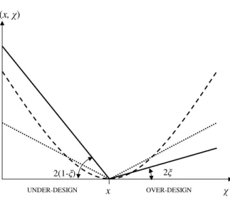
EGU A linear transformation of Eq. (5), obtained by subtractingc·x and dividing byl /2,

ρ_ξ(x, χ)=2ξ(χ ₋x)+2H(x₋χ)_·(x₋χ)

=|χ−x|+2(ξ−0.5)(χ−x). (6)

is a completely equivalent cost-loss function (a similar function is used by Epstein (1969) and by Murphy (1970) when dealing with binary or multicategory variables),

5

but it is more suitable to evaluating predictions. In fact, it depends on a single param-eter, the cost-loss ratioξ=c/l <1, and it attains a null value when χ=x, i.e. when the hypothetical value is equal to the actually occurred one (perfect forecast).

An example of such cost-loss function is reported in Fig. 1, continuous line, where it is compared to an absolute value cost loss-function,ρabs(x, χ)=|x−χ|, and to a quadratic

10

cost-loss function, ρ_quad(x, χ)=(x₋χ)2. The main difference is in the fact that the ρ_ξ function assigns different weights to under-design and to over-design, which is more appropriate when environmental (hydrological) variables are predicted. In this case,ξ values lower than 0.5, giving rise to cost-loss functions similar in shape to the one in Fig. 1, are to be preferred: in fact, the losses are expected to be much greater than the

15

costs of protection. Also note that theρ_ξfunction is the generalization of the absolute value cost-loss function, asρ_ξ converges toρabs when ξ=0.5 (this is another reason

why it is convenient to useρξ rather thanCLfrom Eq.5).

Once the loss function is defined, one can search for the optimal design valueχ∗. By taking the expected value of Eq. (6), one obtains

20

ρξ(χ)=2ξ

χ −

Z

all ˆx

ˆ

xp( ˆx)d ˆx

+2 Z_∞

χ

( ˆx−χ)p( ˆx)d ˆx, (7)

whose derivative with respect toχ, equated to zero, provides the optimal decisionχ∗

P(χ∗)=1₋ξ_⇒χ∗=P−1(1₋ξ) (8)

that depends only on the cumulative distribution function of the forecasts, P(_·), and on the cost loss ratio ξ<1. Of course, the same result would have been obtained by

25

(11)

HESSD

3, 2145–2173, 2006

Title Page

Tables Figures

◭ ◮

Back Close

Full Screen / Esc

EGU using Eq. (5) as the cost-loss function (this is why the two formulations are equivalent).

In contrast, if a similar procedure is adopted with the absolute value or the quadratic cost-loss function (Fig. 1), the median and the mean of the forecasts distribution are respectively selected as the design valuesχ∗.

The total expenses will now amount to ρξ(x, χ∗)=|χ∗−x|+2(ξ−0.5)(χ∗−x), and the

5

operational value of different predictions will be found from the averagedρ(x, χ∗) values over thenpoints in the testing set,

E C(ξ)= 1_n

n

X

i=1

ρξ(xi, χ_i∗)=

1 n

n

X

i=1

n

|P_i−1(1−ξ)−xi|+

2(ξ−0.5)(P_i−1(1−ξ)−x_i)o. (9)

The lower is the obtainedE C(ξ) value (E C stands for “expected cost”), the more

valu-10

able is the forecast. Note that, when the prediction is deterministic,P(x)=H(x−x), and,˜ as mentioned,χ∗=x˜ for anyξ. In this case Eq. (9) reads

E Cdet(ξ)=

1 n

n

X

i=1

{|x˜_i ₋x_i_|+2(ξ₋0.5)( ˜x_i ₋x_i)_}, (10)

which is a discrepancy measure similar to the mean squared error and mean absolute error defined in Eqs. (3) and (4).

15

A difficulty with Eq. (9) is that the expected cost depends on the cost-loss ratioξ; dif-ferent predictions can thus be ranked in different manners by different users, implying that there cannot be an universally accepted “best” probabilistic prediction. This can be especially problematic, since the cost-loss function is seldom known, and, even when it is simplified as in Eq. (6), it may be difficult to set a specific value for the cost-loss

20

(12)

HESSD

3, 2145–2173, 2006

Title Page

Tables Figures

◭ ◮

Back Close

Full Screen / Esc

EGU compared to the costs of the precautionary actions. We also propose to re-scale the

E C(ξ) curves with respect to the cost of a “climatologic” mean-value deterministic pre-diction, ˜x_i=x=1n

Pn

i=1xi. By setting this value in Eq. (10) one obtains that the expected

cost of the climatologic prediction is the mean deviationδ=1n

Pn

i=1|xi−x|. Our proposal

is to plotE C(ξ)/δ versus ξ, in order to be able to directly determine the value of the

5

forecast under analysis compared to the mean-value prediction: if E C(ξ)/δ is lower (larger) than one, the forecast is more (less) valuable than the climatologic prediction. An example of application of this procedure is reported in Sect. 4.

The idea of plotting the E C(ξ) curve is new (however, Palmer, 2000, and Richard-son,2003 use a similar graph for determining the value of probabilistic predictions of

10

discrete variables); more frequently, the meteorologists face the difficulty of setting an exact value forξby supposing thatξis a random variable with a uniformU(0,1) distribu-tion (e.g.,Murphy,1969), and then taking the average value ofE C(ξ) over the possible ξvalues. This corresponds to calculating the areaE Cbelow theE C(ξ) curves,

E C= Z1

0

E C(ξ)dξ= 1_n

n

X

i=1

Z1

0

ρ_ξ(x_i, χ_i∗)dξ. (11)

15

Since the integral and summation terms interchange, we can concentrate on a single addendum in the summation and elide the subscriptsi for simplicity:

T = Z1

0

ρξ(x, χ∗)dξ=

Z1

0{|

P−1(1−ξ)−x|+ (12)

+2(ξ₋0.5)(P−1₍₁

−ξ)₋x)_}dξ.

Substitutingy=P−1(1₋ξ) one has

20

T = Z_∞

−∞{|

y₋x_|+[1₋P(y)](y₋x)_}p(y)dy = Z_∞

−∞

2[H(y₋x)₋P(y)](y ₋x)p(y)dy. (13)

(13)

HESSD

3, 2145–2173, 2006

Title Page

Tables Figures

◭ ◮

Back Close

Full Screen / Esc

EGU Using the formula for integration by parts, and considering thatH(y₋x)₋P(y)=0 when

y→±∞, one obtains

T = Z_∞

−∞

[H(y₋x)₋P(y)]2dy, (14)

i.e. that R1₀ρξ(x, χ∗)dξ is equivalent to the continuous ranked probability score,

CRPS₌R∞_−∞[H(y−x)−P(y)]2dy, which is sometimes used to assess the performances

5

of probabilistic forecasts of continuous variables (Hersbach,2000). As a consequence, E Cin Eq. (11) is also equivalent to CRPS (Hersbach,2000, Eq. 5). This equivalence is not surprising: in fact, the CRPS is the limit of the ranked probability score in Eq. (1) for an infinite numberkof zero-width classes (seeHersbach,2000), and the RPS was obtained by applying to discrete variables a cost-loss function which is similar to ρ_ξ

10

in Eq. (6) (Murphy, 1969, 1970). However, the manner how we obtained the CRPS in Eq. (14) is novel, and allows one to better understand what are its qualities and drawbacks. In particular, Eqs. (12) to (14) demonstrate that the CRPS is averaged over different cost-loss ratios, and, as such, its indications can be misleading, due to the excessive weight assigned in its calculation to expenses correspondent toξvalues

15

larger than 0.5, which are rather unrealistic in the hydrologic field. In our opinion, it is better to evaluate the different predictions by plotting theE C(ξ)/δ curves, rather than trying to summarize all information in a single statistic.

3.2 Statistically-oriented evaluation of probabilistic forecasts

The economists criticize the approach based on the evaluation of the forecasts through

20

the use of cost-loss functions for the fact that the evaluation turns out to be user-dependent rather than objective: in fact, two users with different cost-loss functions may rank in a di_fferent manner two forecasts. Moreover, they argue that the cost-loss function is seldom known, which introduces an undesired element of uncertainty in the evaluation (Diebold et al.,1998). The followed approach is therefore to leave aside

con-25

(14)

HESSD

3, 2145–2173, 2006

Title Page

Tables Figures

◭ ◮

Back Close

Full Screen / Esc

EGU the forecast is correct under a statistical viewpoint. A correct probabilistic forecast ofx_i

is one whose probability density functionpi( ˆxi) coincides with the true distribution ofxi,

f_i(x_i). Even iff_i(x_i) is not known (the distribution changes withi, and only one sampled value is available), it is feasible to build up a test of the hypothesisH0 :pi( ˆxi)≡fi(xi).

The test is based on the probability integral transform,zi=Pi(xi), that consists in

eval-5

uating the cumulative distribution function of the predictions in correspondence to the observed value x_i (Berkovitz, 2001). Under the hypothesis H0, the distribution of zi

is uniform, U(0,1). If one applies the probability integral transform to all points in the testing set, a sample ofz_i values is obtained. If the probability forecast is correct, the z_i values are mutually independent and identically U(0,1) distributed. The test of the

10

hypothesisH0 can therefore be split into an independence test and a goodness-of-fit

test of theU(0,1) hypothesis.

As for the independence, the usual suggestion is to look at the autocorrelation func-tion of thezi’s and of their powersz

2 i, ..., z

m

i (e.g.,Diebold et al.,1998). This produces

some proliferation of the test statistics (one for each considered power), with possible

15

problems of interpretation of the results. Our proposal is to use instead the Kendall’s τtest of independence (Kendall and Stuart,1977). Consider the sequencez1, ..., zn,

and their associated ranksR1, ..., Rn, i.e. their position in the ordered vector of thezi’s.

Kendall’sτtest of independence is based on the statistic

τ=1₋ 4Nd

(n−1)(n−2), (15)

20

where N_d is the number of discordances, i.e. the number of pairs (R_i, R_i₊₁) and (Rj, Rj+1) that satisfy eitherRi<Rj andRi+1>Rj+1, orRi>Rj andRi+1<Rj+1.

Under the null hypothesis of independent values and with n>10, the standardized statistic

τst =

τ σ_τ =τ·

s

9n(n−1)

2(2n+5) (16)

25

(15)

HESSD

3, 2145–2173, 2006

Title Page

Tables Figures

◭ ◮

Back Close

Full Screen / Esc

EGU has a normal distribution with null mean and unitary variance (Kendall and Stuart,

1977), which allows one to easily determine the limit values for the independence test. For example, the 95% test of independence will be passed ifτstis below 1.645 (one-tail

test).

Consider now the uniformity hypothesis: many goodness-of-fit tests for this

hypothe-5

sis exist (D’Agostino and Stephens,1986;Noceti et al.,2003). However,Diebold et al. (1998) argue that it is better to adopt a less formal graphical method, based on an histogram representation of the density of thezi’s. We agree that the graphical

repre-sentation is more revealing, but prefer a probability plot reprerepre-sentation that does not require a subjective binning of the data. The probability plot is a plot of thez_i values

10

versus their empirical cumulative distribution function,Ri/n. The shape of the

result-ing curve reveals if the data are approximatively uniform, in which case the (z_i, R_i/n) points are close to the bisector of the diagram. Kolmogorov confidence bands can also be represented on the same graph in order to provide a more formal test of uniformity. The Kolmogorov bands are two straight lines, parallel to the bisector and at a distance

15

q(α)/√nfrom it, where q(α) is a coefficient, dependent upon the significance level of the testα (e.g., q(α=0.05)=1.358, see D’Agostino and Stephens,1986). The test is passed when the curves remain inside these confidence bands.

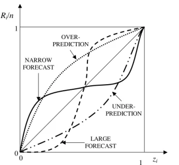
The probability plot representation does not only tell if the uniformity test is passed or not, but also provides a tool to investigate the causes behind deviations from uniformity.

20

In fact, the shape of the curves in the probability plot (see Fig. 2) is suggestive of the encountered problem, since the steepness of the curves is larger where morez_i points concentrate. In the case of the continuous line in Fig. 2, for example, thezi points are

concentrated in the vicinity of the end points 0 and 1. This corresponds to having the real x_i values that fall, more frequently than expected, on the tails of the distribution

25

(16)

HESSD

3, 2145–2173, 2006

Title Page

Tables Figures

◭ ◮

Back Close

Full Screen / Esc

EGU for the verification of probabilistic predictions of binary variables.

When using this approach to forecast verification, one ends out with results concern-ing with the formal correctness of the probabilistic prediction; however, these results do not imply that the prediction is good: there can exist a prediction that passes the inde-pendence and uniformity tests, but has no operational value. In our opinion, the method

5

should therefore necessarily be used together with some other method, like those de-scribed in Sect. 3.1, allowing one to understand if the prediction is really valuable or not.

A final comment is necessary regarding multi-step-ahead predictions (i.e., char-acterized by a prediction horizon h₆=1). In this case, serial correlation in the z_i

10

series is expected up to a lag h−1 (Box and Jenkins, 1970), and the indepen-dence and goodness-of-fit tests should be applied separately to the h subseries

{z1, z1+h, z1+2h, ...},{z2, z2+h, z2+2h, ...}, ...,{zh, z2h, z3h, ...}(Diebold et al.,1998). One

obtainsh τst statistics andhprobability plots for each prediction. The global tests will

be obtained from the combination of the tests performed on each of the subseries:

15

however, the combination is complicated by the fact that thehsubseries are mutually (not internally!) dependent. When the samples being tested are correlated, the correct significance level to have a globalα-level test should be betweenα(linearly dependent samples) andα/h(independent samples). In our opinion the correlation between the subseries is strong, and it is thus better to perform the tests on thehsubseries with

20

a significance levelα, instead of using a levelα/hfor each sub-test as suggested by Diebold et al.(1998).

4 Application and discussion

The verification tools described in the previous sections are applied to the probabilis-tic forecasts of a discharge time series, obtained with a prediction method developed

25

(17)

HESSD

3, 2145–2173, 2006

Title Page

Tables Figures

◭ ◮

Back Close

Full Screen / Esc

EGU byTamea et al. (2005) and Laio et al. (2006)1and based on local polynomial

regres-sion techniques (Farmer and Sidorowich,1987;Fan and Gijbels,1996;Cleveland and Loader,1996;Porporato and Ridolfi,1997;Regonda et al.,2005). We use this predic-tion method as a mean to exemplify the described verificapredic-tion techniques. We therefore refer toTamea et al. (2005) and Laio et al. (2006)1 for a description of the prediction

5

method, and concentrate on the scope of the present work, which is the analysis of the forecast verification tools. For the comprehension of the following of the paper it is suf-ficient to consider here the prediction as the outcome of a black-box method, requiring as an input the time series of past values of discharge (and concurring average precip-itation over the basin). The method produces predictions for the points in the testing

10

set, provided that a set_S of model parameter values is assigned by the forecaster. We use in our verification exercise four di_fferent types of predictions, all based on the mentioned local polynomial regression method. Two forecasting techniques are deterministic and two are probabilistic, as detailed hereafter.

1. Best deterministic prediction: it is the point forecast obtained by selecting the

15

parameter set Sbest that produces the “best” deterministic predictions when the

method is applied to the calibration set, i.e. to a set of discharge values selected for cross-validation purposes (seeTamea et al.,2005).

2. Ensemble forecast: it is a probabilistic forecast obtained by selecting, through cross-validation,qparameter sets rather than a single one (we use in the following

20

exampleq=100). Each of these sets is separately used in the prediction method, obtainingqdifferent predictions for each pointxi in the testing set. The empirical

distribution function of this sample of q predictions is taken as representative of the distribution characterizing the ensemble forecast.

3. Probabilistic forecast: the same as before, but with a suitable parameter

uncer-25

1

(18)

HESSD

3, 2145–2173, 2006

Title Page

Tables Figures

◭ ◮

Back Close

Full Screen / Esc

EGU tainty representation attached to each member in the ensemble. This is obtained

by using thek residuals of the local polynomial regressions (k is one of the pa-rameters belonging to theS set); these residuals are opportunely converted into out-of-sample errors and then summed up to the point predictions in the ensemble (seeTamea et al.,2005, and Laio et al., 20061). A large sample of ˆxi ,j,j=1, .., q·k

5

values is obtained, whose empirical distribution function is taken as the estimate ofp_i( ˆx_i).

4. Median prediction: it is a deterministic prediction obtained by taking, for each point in the testing set, the median of the above defined probabilistic prediction p_i( ˆx_i) as the estimator of ˜x_i.

10

The prediction methods have been applied to the discharge time series of the Tanaro river, in the northwest of Italy. The catchment basin at the gauge station of Farigliano has an extension of 1522 km2 and an elevation ranging from 235 to 2651 m above the sea level. The hourly discharge time series has been measured from 1997 to 2002. The testing set covers the period between 14 November 2002 and 27 November 2002,

15

and corresponds to an important flood event. The mean rainfall over the catchment is used as an endogenous variable for the prediction. The mean rainfall is determined from the data collected by eleven rain gauges located on the basin. Both hydrometric and pluviometric data have been collected by the Regional Agency for the Protec-tion of the Environment (ARPA-Piemonte), and are the same already used byTamea

20

et al. (2005) (we refer to that paper for a graphical representation of the prediction out-comes). Prediction horizons of one and six hours (corresponding toh=1 andh=6) are considered in the following examples.

In Fig. 3 the expected cost from Eq. (9), re-scaled by using the mean deviationδ, is represented as a function of the cost-loss ratioξ for the four predictions listed above.

25

Note that theE C(ξ)/δvalues are much lower than 1, both for the 1-h ahead prediction (Fig. 3a) and for the 6-h ahead prediction (Fig. 3b), demonstrating that all forecasting methods are very competitive with respect to the climatological prediction. The quality

(19)

HESSD

3, 2145–2173, 2006

Title Page

Tables Figures

◭ ◮

Back Close

Full Screen / Esc

EGU of the four prediction methods can now be comparatively evaluated: the lower is the

expected cost of a forecast, the higher is its operational value. It is clear from Fig. 3 that the two probabilistic methods outperform the deterministic ones, in particular in the part of the diagram that is more important when dealing with flood events (large expected losses compared to the costs, i.e. lowξvalues).

5

It is also interesting to comment on the shape of the four curves in the diagram: the relation between the expected cost and ξ turns out to be linear when the prediction is deterministic; in fact, by setting P_i−1(1₋ξ)=x˜i in Eq. (9), one obtains the equation

of a straight line, whose slope is two times the bias of the prediction, _n1Pn_i₌₁( ˜x_i−x_i), and whose intercept with theξ=0.5 vertical line is the MAE of the forecast, a measure

10

of the spread of the prediction errors. As expected, both the (negative) bias and the spread of the errors increase when the prediction horizon passes from 1 to 6 h. The median prediction is better than the best deterministic prediction forξ<0.5, which is mainly due to the beneficial e_ffect of taking an ensemble of predictions rather than a single one (seeGeorgakakos et al.,2004;Tamea et al.,2005;Regonda et al.,2005).

15

On the same diagram the probabilistic predictions tend to have a parabolic shape, with null (or very low) values at the extremes and a maximum forξ≈0.5. The reason for the low values at the extremes is the following: whenξ=0 the cost of the precaution-ary actions is null, and one can therefore always take an action that protects against any possible occurring flood. Analytically, whenξ=0, one hasP_i−1(1₋ξ)=max( ˆxi) and

20

E C(ξ=0)=1n

Pn

i=1{|max( ˆxi)−xi|−(max( ˆxi)−xi)}; the only terms contributing to the

ex-pected cost are therefore those when the actually occurred valuex_i is greater than the maximum predicted value, max( ˆxi), which never happens for the more reliable

proba-bilistic prediction, and only rarely for the ensemble prediction.

When ξ=1 the cost of the precautionary action is equal to that of the eventually

25

occurring losses; there is thus no convenience to take any action, i.e. the design value χ in Eq. (6) can be set to zero (actually, to min( ˆxi)). As a consequence, ρξ=1 and

(20)

HESSD

3, 2145–2173, 2006

Title Page

Tables Figures

◭ ◮

Back Close

Full Screen / Esc

EGU this fictitious result. However, this is not a relevant incongruence, since both extremes

ξ=0 and ξ=1 correspond to unrealistic situations when the decision to be taken is obvious, and the forecast is useless. It is not then the shape of the single curve on the diagram that is of interest, but the relations between the curves for fixedξ values. Considering this aspect, it can be noted how the probabilistic prediction provides more

5

valuable results than the ensemble prediction, in particular for the more relevant lowξ values.

As a further detail, the continuous ranked probability score values are the follow-ing: ath = 1, CRPS=10.1 m3/s for the best deterministic prediction, CRPS=8.8 m3/s for the ensemble prediction, CRPS=7.7 m3/s for the probabilistic prediction, and

10

CRPS=10.2 m3/s for the median prediction. At h=6, the corresponding values are 41.7 m3/s (best), 25.8 m3/s (ensemble), 23.6 m3/s (probabilistic), and 31.1 m3/s (me-dian). These values correspond to the areas below the curves in Fig. 3, multiplied by the mean deviationδ=181.7 m3/s. Also these results confirm the superiority of the probabilistic method, even if, as mentioned, the relevance of the CRPS index is doubtful

15

when dealing with hydrological applications.

We now turn to the application of the statistically-oriented forecast verification tools: since these methods are targeted at evaluating probabilistic predictions only, the com-parison will be limited to the ensemble and probabilistic predictions methods. As men-tioned, the verification of the probabilistic forecast is a two step process, requiring to

20

apply the transformationzi=Pi(xi) and then separately test the independence and the

uniformity of thez_i’s. The standardized Kendall’sτst statistic in Eq. (16) is calculated,

obtainingτst=1.38 (ensemble) andτst=−3.17 (probabilistic) for h=1. Both values are

not significant at the 5% level, i.e. the independence test is passed. For h=6, six subseries{z1, z7, z13, ...},{z2, z8, z14, ...}, ...,{z6, z12, z18, ...}are constructed, and six

25

differentτstvalues (for each prediction) are obtained. The independence test is passed

if the maximum among these values is not significant at theα level. The obtained val-ues are τst=3.11 (ensemble) and τst=0.90 (probabilistic), i.e. the independence test

(21)

HESSD

3, 2145–2173, 2006

Title Page

Tables Figures

◭ ◮

Back Close

Full Screen / Esc

EGU diction (note that the test would not be passed even when the significance level was

reduced toα/h=0.008, as suggested byDiebold et al.,1998).

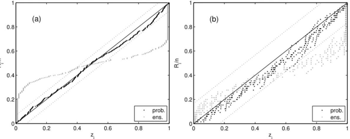
The uniformity of the z_i’s is then verified by plotting the data versus their empirical cumulative distribution (see Fig. 4). Using Fig. 2 as a guide to evaluate the results, it is clear that the ensemble method provides predictions that are very narrow around the

5

central value. In contrast, the forecasts obtained through the probabilistic method are very reliable (the points remain inside the Kolmogorov bands with 5% significance). A (slight) negative bias is detected ath=6 (Fig. 4b), as apparent from the fact that the points lie below the bisector of the diagram (compare to Fig. 2). The results forh=6 refer to six different curves, due to the mentioned separation of the testing set in six

10

subseries. The Kolmogorov bands are larger in Fig. 4b with respect to Fig. 4a for that same reason; in fact, when testing separately the 6 sub-series, the actual size of the samples isn/6 and the acceptability limits become larger.

5 Conclusions

We have here compared different strategies for evaluating the performances of

prob-15

abilistic prediction methods of continuous variables. All analyzed methods have some interesting characteristics, but none of them, taken alone, allows a complete and fair evaluation of the quality of the forecast. Our suggestion is to use two methods together, as each carries a fundamental information about the prediction quality. More in detail, the expected cost diagram (Fig. 3) is a very useful tool to understand the operational

20

value of the forecast, especially when comparing different (deterministic and proba-bilistic) predictions. This approach, however, does not provide sufficient information for a complete evaluation: in fact, the reliability of the forecast, i.e. the fact that the distri-bution of the predictions,p_i( ˆx_i), is equal to the real distribution,f_i(x_i), is hypothesized rather than verified (see Sect. 3). Moreover, the definition of a cost-loss function always

25

demands some subjective choice: for example, we have takenρξin Eq. (6) to be

(22)

HESSD

3, 2145–2173, 2006

Title Page

Tables Figures

◭ ◮

Back Close

Full Screen / Esc

EGU do not think that the outcomes of the forecast verification would qualitatively change

when using a quadratic cost-loss function, but in any case we believe that it is nec-essary to complement the expected cost curve with other tools, aimed at verifying the statistical congruence of the forecast, i.e. the hypothesis thatp_i( ˆx_i)=f_i(x_i). More in de-tail, we found that suitable tools, based on the probability integral transformzi=Pi(xi),

5

require the application of the Kendall’s independence test and the representation of the z_i’s through a probability plot (Fig. 4), which allows one to assess the uniformity of the zi’s. The combination of these two approaches, respectively based on the concept of

operational value of the forecast and on the formal statistical verification of its reliability, provides the basis for an exhaustive and effective probabilistic forecast evaluation.

10

Acknowledgements. We are grateful to L. Ridolfi for his helpful suggestions and comments during the course of this research.

References

Abramson, B. and Clemen, C.: Probability forecasting, Int. J. Forecast., 11, 1–4, 1995. 2148

Berkovitz, J.: Testing density forecasts, with applications to risk management, J. Bus. Econ. 15

Stat., 19, 465–474, 2001. 2152,2158

Beven, K.: A manifesto for the equifinality thesis, J. Hydrol., 320, 18–36, doi:10.1016/j.jhydrol.

2005.07.007, 2006. 2146

Box, G. E. P. and Jenkins, G. M.: Time series analysis: forecasting and control, Holden Day,

San Francisco, CA, 1970. 2160

20

Chatfield, C.: Prediction intervals for time series forecasting, in: Principles of forecasting: a handbook for researchers and practitioners, edited by: Armstrong, J., p. 475–494, Kluwer

Academic Publishers, Norwell, MA, 2001. 2148

Christoffersen, P. F.: Evaluating interval forecast, Int. Econ. Rev., 39, 841–862, 1998. 2148,

2151

25

Cleveland, W. S. and Loader, C. L.: Smoothing by Local Regression: Principles and Methods, in: Statistical Theory and Computational Aspects of Smoothing, edited by: Haerdle, W. and

Schimek, M. G., p. 10–49, Springer, New York, 1996. 2161

(23)

HESSD

3, 2145–2173, 2006

Title Page

Tables Figures

◭ ◮

Back Close

Full Screen / Esc

EGU

D’Agostino, R. B. and Stephens, A. M. (Eds.): Goodness-of-fit techniques, Dekker, New York,

1986. 2159

De Gooijer, J. G. and Zerom, D.: Kernel-based multistep-ahead predictions of the US short-term interest rate, J. Forecast., 19, 335–353, 2000. 2159

Diebold, F. X., Gunther, T. A., and Tay, A. S.: Evaluating density forecasts with applications to 5

financial risk management, Int. Econ. Rev., 39, 863–883, 1998. 2147,2152,2153, 2157,

2158,2159,2160,2165

Epstein, E. S.: A scoring system for probability forecasts of ranked categories, J. Appl.

Meteo-rol., 8, 985–987, notes and correspondence, 1969. 2149,2152,2154

Fan, J. and Gijbels, I.: Local polynomial modelling and its applications, Chapman and Hall, 10

London, UK, 1996. 2161

Farmer, J. D. and Sidorowich, J. J.: Predicting chaotic time series, Phys. Rev. Lett., 59, 845–

848, 1987. 2161

Ferraris, L., Rudari, R., and Siccardi, F.: The uncertainty in the prediction of flash floods in the

Northern Mediterranean Environment, J. Hydrometeorol., 3, 714–727, 2002. 2146

15

Gangopadhyay, S., Clark, M., and Rajagopalan, B.: Statistical downscaling using K-nearest

neighbors, Water Resour. Res., 41, W02024, doi:10.1029/2004WR003444, 2005. 2146

Georgakakos, K. P., Seo, D.-J., Gupta, H., Schaake, J., and Butts, M. B.: Towards the char-acterization of streamflow simulation uncertainty through multimodel ensembles, J. Hydrol., 298, 222–241, doi:10.1016/j.jhydrol.2004.03.037, 2004. 2146,2147,2163

20

Goodman, L. A. and Kruskal, W. H.: Measures of association for cross classifications, J. Am.

Stat. Assoc., 49, 732–764, 1954. 2149

Hersbach, H.: Decomposition of the continuous ranked probability score for ensemble

predic-tion systems, Weather and Forecasting, 15, 559–569, 2000. 2157

Jolliffe, I. T. and Stephenson, D. B. (Eds.): Forecast verification: a practitioner’s guide in atmo-25

spheric science, Wiley, New York, USA, 2003. 2147,2149

Kendall, M. G. and Stuart, A.: The advanced theory of statistics, Griffin Press, London, 2nd ed., 1977. 2149,2158,2159

Krzysztofowicz, R.: The case for probabilistic forecasting in hydrology, J. Hydrol., 249, 2–9,

2001. 2146

30

Montanari, A.: Large sample behaviors of the generalized likelihood uncertainty estimation (GLUE) in assessing the uncertainty of rainfall-runoffsimulations, Water Resour. Res., 41,

(24)

HESSD

3, 2145–2173, 2006

Title Page

Tables Figures

◭ ◮

Back Close

Full Screen / Esc

EGU

Montanari, A. and Brath, A.: A stochastic approach for assessing the uncertainty of

rainfall-runoff simulations, Water Resour. Res., 40, W01106, doi:10.1029/2003WR002540, 2004.

2146

Murphy, A. H.: Measures of the utility of probabilistic predictions in cost-loss ratio decision situation in which knowledge of the cost-loss ratio is incomplete, J. Appl. Meteorol., 8, 863– 5

873, 1969. 2151,2152,2156,2157

Murphy, A. H.: The ranked probability score and the probability score: a comparison, Mon.

Wea. Rev., 98, 917–924, 1970. 2149,2150,2154,2157

Murphy, A. H.: A note on the ranked probability score, J. Appl. Meteorol., 10, 155–156, 1971.

2149

10

Noceti, P., Smith, J., and Hodges, S.: An evaluation of tests of distributional forecasts, J.

Fore-cast., 22, 447–455, 2003. 2152,2159

Palmer, T. N.: Predicting uncertainty in forecasts of weather and climate, Rep. Progr. Phys., 63,

71–116, 2000. 2151,2153,2156

Porporato, A. and Ridolfi, L.: Nonlinear analysis of river flow time sequences, Water Resour. 15

Res., 33, 1353–1367, 1997. 2161

Regonda, S., Rajagopalan, B., Lall, U., Clark, M., and Moon, Y.: Local polynomial method for

ensemble forecast of time series, Nonlin. Processes Geophys., 12, 397–406, 2005. 2161,

2163

Richardson, D. S.: Economic value and skill, in: Forecast verification: a practitioner’s guide in 20

atmospheric science, edited by: Jolliffe, I. T. and Stephenson, D. B., Wiley, New York, USA, 2003. 2146,2151,2153,2156

Siccardi, F., Boni, G., Ferraris, L., and Rudari, R.: A hydrometeorological approach for prob-abilistic flood forecast, J. Geophys. Res., 110, D05101, doi:10.1029/2004JD005314, 2005.

2146

25

Tamea, S., Laio, F., and Ridolfi, L.: Probabilistic nonlinear prediction of river flows, Water

Re-sour. Res., 41, W09421, doi:10.1029/2005WR004136, 2005. 2146,2161,2162,2163

Tay, A. S. and Wallis, K. F.: Density forecasting: a survey, J. Forecast., 19, 235–254, 2000.

2148

Todini, E.: Role and treatment of uncertainty in real-time flood forecasting, Hydrol. Processes, 30

18, 2743–2746, 2004. 2146

Wilks, D. S.: Statistical methods in the atmospheric sciences, Academic press, 1995. 2147,

2148,2149,2150,2151,2159

(25)

HESSD

3, 2145–2173, 2006

Title Page

Tables Figures

◭ ◮

Back Close

Full Screen / Esc

EGU

Table 1.Forecast verification tools, subdivided by the type of predicted variable (columns) and the forecast outcome (rows). We refer to Sect. 2 for details and references about the methods.

Discrete predictands Multicategory Binary

Nominal Ordinal

Continuous Predictands

Deterministic forecast

HIT RATE, THREAT SCORE, …

PEARSON’S COEFF. OF CONTINGENCY

GOODMAN AND KRUSKAL

G STATISTIC

MSE MAE

Interval forecast NOT APPLICABLE

NOT APPLICABLE

TESTS FOR THE CONDITIONAL AND UNCOND. COVERAGE

Probabilistic

forecast BRIER SCORE

CONVERSION TO BINARY

TABLES

RANKED PROBABILITY

SCORE

(26)

HESSD

3, 2145–2173, 2006

Title Page

Tables Figures

◭ ◮

Back Close

Full Screen / Esc

EGU x OVER-DESIGN

UNDER-DESIGN _χ

2

ρ(x, χ)

2(1- )

zi

R

Fig. 1.Examples of quadratic (dashed line), absolute-value (dotted line) and asymmetric (con-tinuous line, see Eq.6) cost-loss functions. The variableχon the horizontal axis is the “design” value, whilexis the real future value.

(27)

HESSD

3, 2145–2173, 2006

Title Page

Tables Figures

◭ ◮

Back Close

Full Screen / Esc

EGU 0

1

1 OVER-

PREDICTION

UNDER- PREDICTION

LARGE FORECAST NARROW

FORECAST

zi Ri/n

0

(28)

HESSD

3, 2145–2173, 2006

Title Page

Tables Figures

◭ ◮

Back Close

Full Screen / Esc

EGU

0 0.2 0.4 0.6 0.8 1

0 0.01 0.02 0.03 0.04 0.05 0.06 0.07

cost−loss ratio, ξ

expected cost, EC(

ξ

)/

δ

(a)

best.det. median ens. prob.

0 0.2 0.4 0.6 0.8 1

0 0.05 0.1 0.15 0.2 0.25 0.3

cost−loss ratio, ξ

expected cost, EC(

ξ

)/

δ

(b)

best.det. median ens. prob.

Fig. 3. Representation of the expected cost from Eq. (9) (re-scaled by the mean deviationδ) as a function of the cost-loss ratioξ, for a 1 step-ahead (a) and a 6-steps ahead(b)hourly discharge prediction. The four lines in each graph refer to four different forecasting methods, described at the beginning of Sect. 4.

(29)

HESSD

3, 2145–2173, 2006

Title Page

Tables Figures

◭ ◮

Back Close

Full Screen / Esc

EGU

0 0.2 0.4 0.6 0.8 1

z i

Ri

/n

(a)

prob. ens.

0 0.2 0.4 0.6 0.8 1

z i

Ri

/n

(b)

prob. ens.