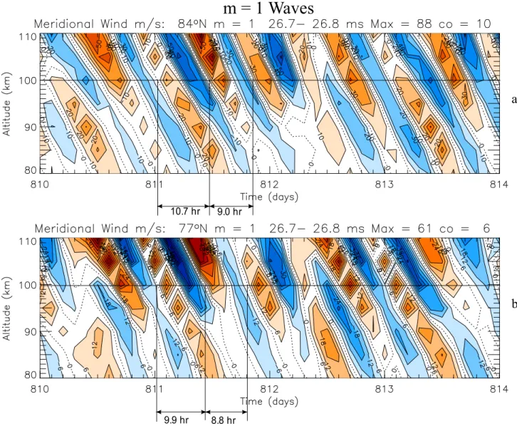
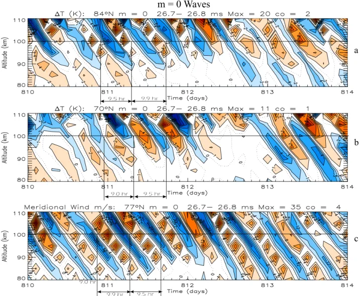
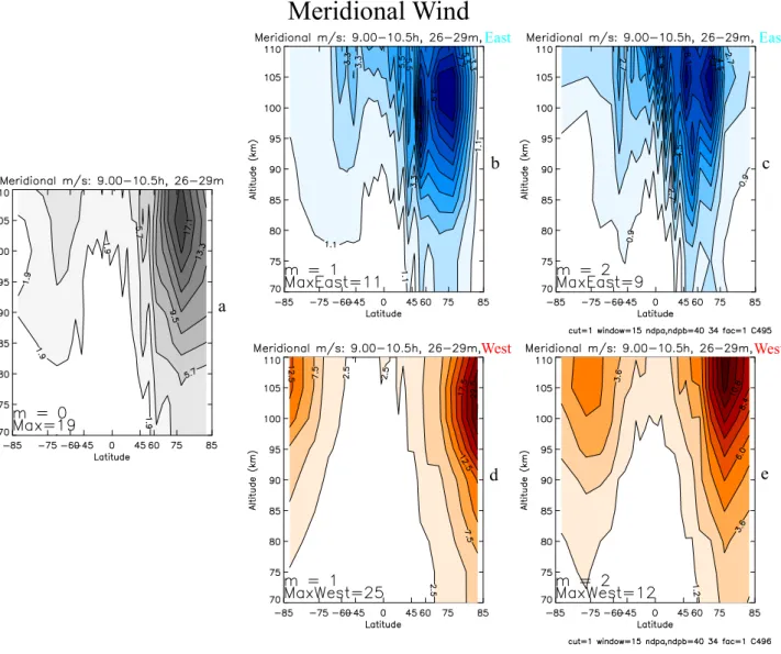
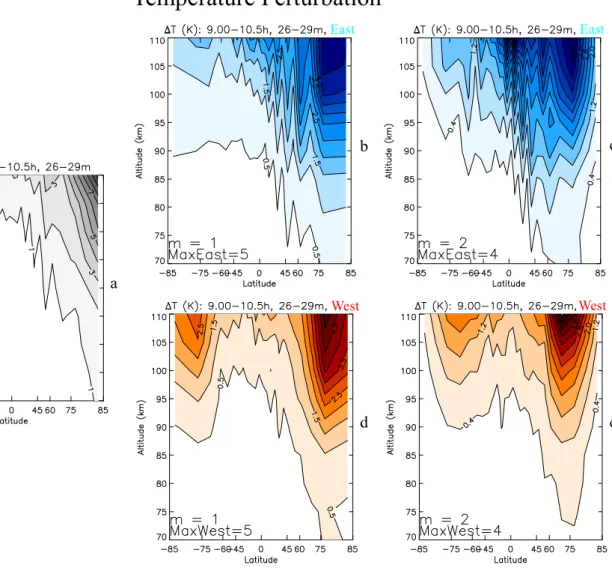
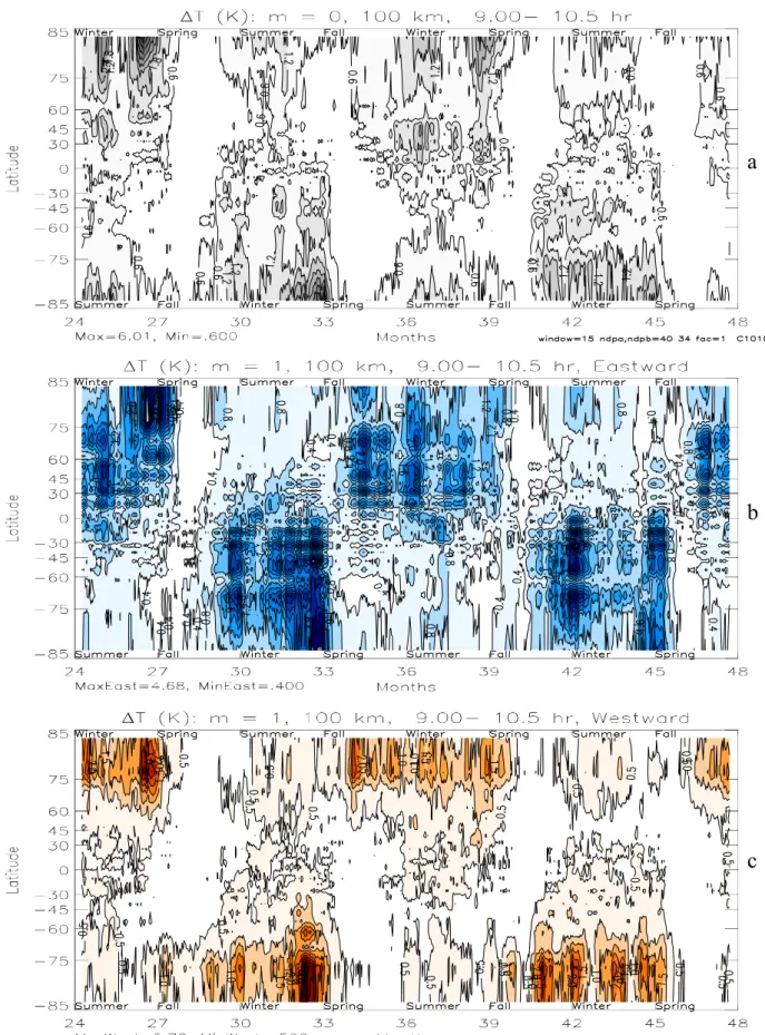
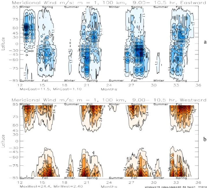
Properties of internal planetary-scale inertio gravity waves in the mesosphere

Além disso, o Facebook também disponibiliza várias ferramentas exclusivas como a criação de eventos, de publici- dade, fornece aos seus utilizadores milhares de jogos que podem

Na hepatite B, as enzimas hepáticas têm valores menores tanto para quem toma quanto para os que não tomam café comparados ao vírus C, porém os dados foram estatisticamente

i) A condutividade da matriz vítrea diminui com o aumento do tempo de tratamento térmico (Fig.. 241 pequena quantidade de cristais existentes na amostra já provoca um efeito

Peça de mão de alta rotação pneumática com sistema Push Button (botão para remoção de broca), podendo apresentar passagem dupla de ar e acoplamento para engate rápido

Neste trabalho o objetivo central foi a ampliação e adequação do procedimento e programa computacional baseado no programa comercial MSC.PATRAN, para a geração automática de modelos

Ousasse apontar algumas hipóteses para a solução desse problema público a partir do exposto dos autores usados como base para fundamentação teórica, da análise dos dados

Despercebido: não visto, não notado, não observado, ignorado.. Não me passou despercebido

Caso utilizado em neonato (recém-nascido), deverá ser utilizado para reconstituição do produto apenas água para injeção e o frasco do diluente não deve ser