Universidade Federal de Minas Gerais
Instituto de Ciˆ
encias Exatas
Departamento de Matem´
atica
Tese de doutorado
Sobre o funcional de a¸c˜
ao m´ınima de
Mather: propriedades gen´
ericas e
diferenciabilidade
Alexandre Alvarenga Rocha
Orientador: M´ario Jorge Dias Carneiro
On the Mather’s minimal action
functional: Generic properties and
differentiability
Alexandre Alvarenga Rocha
Advisor: M´ario Jorge Dias Carneiro
Alexandre Alvarenga Rocha
Sobre o funcional de a¸c˜
ao m´ınima de
Mather: propriedades gen´
ericas e
diferenciabilidade
Tese apresentada ao Programa de P´os-Gradua¸c˜ao em Matem´atica da Universidade Federal de Mi-nas Gerais, como requisito parcial para obten¸c˜ao do t´ıtulo de Doutor em Matem´atica
Orientador: M´ario Jorge Dias Carneiro
`
Agradecimentos
Ao meu orientador M´ario Jorge pelos ensinamentos.
Aos meus pais Humberto e Maria Socorro e ao meu irm˜ao Carlos pelo incentivo e apoio. `
A minha namorada Gabriela pela paciˆencia e companheirismo.
Aos meus amigos de trabalho (UFV-Campus Florestal) por todo apoio dado durante o treinamento.
Aos meus amigos de Florestal e da p´os gradua¸c˜ao da UFMG.
Resumo
Nesta tese, apresentamos algumas propriedades gen´ericas e suas consequˆencias na dinˆamica do conjunto de Aubry, o qual aparece na Teoria de Mather sobre La-grangianos de Tonelli e sistemas Hamiltonianos. Tamb´em estudamos condi¸c˜oes para diferenciabilidade do funcional de a¸c˜ao m´ınima de Mather e algumas implica¸c˜oes de sua regularidade na dinˆamica do sistema.
Na primeira parte, provamos que, no conjunto de Lagrangianos Magn´eticos Exa-tos, a propriedade “Existem finitas classes est´aticas para toda classe de cohomologia” ´e gen´erica. Obtemos tamb´em algumas consequˆencias dinˆamicas dessa propriedade.
Na segunda parte, apresentamos uma condi¸c˜ao dinˆamica de modo a obter diferen-ciabilidade da fun¸c˜ao β de Mather. Mais precisamente, n´os obtemos diferenciabilidade deβ em todas as classes de homologia correspondentes aos vetores de rota¸c˜ao de medi-das cujos suportes est˜ao contidos em um gr´afico Lagrangiano Lipschitz, invariante por Hamiltonianos de Tonelli. Tamb´em mostramos a rela¸c˜ao entre diferenciabilidade local deβ e integrabilidade local do fluxo Hamiltoniano.
Na ´ultima parte, mostramos um exemplo de uma fun¸c˜ao β de Mather definida sobre o grupo de homologia do toro T2, usando os resultados obtidos sobre sua dife-renciabilidade.
Abstract
In this thesis we present some generic properties and its consequences to the dy-namics of the Aubry set that appear in the Mather’s theory about Tonelli Lagrangians and Hamiltonian systems. We also study conditions for differentiability of the Mather’s minimal action functional and some implications of its regularity to the dynamics of the system.
In the first part, we prove that for the set of exact magnetic Lagrangians, the property “There exist finitely many static classes for every cohomology class” is generic. We also obtain some dynamical consequences of this property.
In the second part, we present a dynamical condition in order to obtain differ-entiability of Mather’s β-function. More preciselly, we obtain differentiability of β
on all homology classes corresponding to rotation vectors of measures whose supports are contained in a Lipschitz Lagrangian absorbing graph, invariant by Tonelli Hamil-tonians. We also show the relationship between local differentiability of β and local integrability of the Hamiltonian flow.
In the last part, we show an example of Mather’s β-function on the homology group of two torus T2, by using the results obtained about its differentiability.
Contents
1 Introduction 7
2 Preliminaries 12
2.1 Tonelli Lagrangians and Hamiltonians . . . 12
2.2 Mather, Aubry and Ma˜n´e sets . . . 13
2.3 Functionsα and β of Mather . . . 14
3 A generic property of exact magnetic Lagrangians 17 3.1 Adapting the abstract setting of Bernard and Contreras . . . 17
3.2 Some dynamical consequences . . . 24
3.3 Finitely many hyperbolic periodic orbits for a generic magnetic Lagrangian 26 3.4 Example . . . 29
3.5 Questions . . . 31
4 A dynamical condition for differentiability of Mather’s average action 32 4.1 Aubry and Ma˜n´e sets and Hamilton-Jacobi equation . . . 32
4.2 Absorbing sets . . . 34
4.3 Proof of Theorems 1.5 and 1.6 . . . 37
4.4 Dynamical properties on a neighborhood of graphs and differerentiability of β . . . 40
4.5 The case M =T2 . . . 44
4.6 A non-absorbing graph . . . 46
4.7 Another weak integrability condition for the case M =T2 . . . 48
4.8 Questions . . . 54
5 Example: exact magnetic Lagrangians 55 5.1 Ma˜n´e’s critical value . . . 55
5.2 A special case of vertical exact magnetic Lagrangian . . . 57
5.2.1 Symmetry of the functions α and β of Mather . . . 58
CONTENTS 6
5.2.2 Flats of Mather’sα-function . . . 61 5.2.3 Local differentiability of the functionsα and β of Mather . . . . 63
Chapter 1
Introduction
Let M be a compact connected manifold equipped with a Riemannian metric
g =⟨., .⟩ andT M its tangent bundle. A Tonelli Lagrangian is a function L:T M →R of class at leastC2 which is convex and superlinear when restricted to any fiber. This
special type of Lagrangian fits into Mather’s theory, as developed by R. Ma˜n´e and A. Fathi in different ways.
The Euler-Lagrange equation associated to a Lagrangian L defines a complete flow φL
t,called Euler-Lagrange flow. Let us recall the main concepts introduced by J.
Mather in [24]. Let M(L) be the set of probabilities on the Borel σ-algebra on T M
which are invariant under the Euler–Lagrange flow φL
t. The action of a measure µin
M(L), is defined by
AL(µ) =
∫
T M
L dµ.
Let M(L) be the set of action minimizing measures, i.e. the set of Borel
prob-ability measures µ on T M which are invariant under the Euler-Lagrange flow φL t
ge-nerated by L and minimize the action, that is, for all invariant probability ν on T M,
AL(µ)≤AL(ν).
The ergodic components of a minimizing measure are also minimizing and the setM(L) is a simplex whose extremal points are the ergodic minimizing measures.
The Euler-Lagrange flow generated by L does not change by adding a closed one-form ζ and, given µ ∈ M(L), Mather proves that ∫T Mdf(x).v dµ = 0 for each
f ∈C1(M).Therefore the action L−ζ of a probability measure µ∈ M(L), depends
only on the cohomology class c= [ζ] ∈H1(M;R) and we can also consider the set of
action minimizing measures M(L−c). Moreover, the minimal action value depends
only on the cohomology class c = [ζ] ∈ H1(M;R) of the closed one-form, so it is
8
denoted by −α(c). More precisely,
α(c) =− inf
µ∈M(L)AL−c(µ).
Mather proved that the function c 7→ α(c), so-called Mather’s α-function, is convex and superlinear. It is known that α(c) is the value of the energy level that contains the Mather set of cohomology class c:
f
Mc =
∪
µ
supp(µ),
where the union is taken over the set of Borel probability measures µ ∈ M(L−c).
The set Mfc is a compact invariant set which is a graph over a compact subsetMc of
M, the projected Mather set (see [24]). Mc is laminated by curves, which are global
(or time independent) minimizers.
In general,Mfcis contained in another compact invariant set, which is also a graph
whose projection is laminated by global minimizers: the Aubry set for the cohomology class c, denoted byAec. Ma˜n´e proved that Aec is chain recurrent and it is a challenging
question to describe the dynamics of the Euler-Lagrange flow restricted to Aec ⊂T M.
The definitions of the Aubry set and its dual A∗
c ⊂T∗M are given in Chapter 2.
Generic properties
A LagrangianL is called exact magnetic Lagrangian if
L(x, v) = ∥v∥
2
2 +⟨η, v⟩ (1.1) for some non-closed 1-formη. This type of Lagrangian fits into Mather’s theory about Tonelli Lagrangians, because it is fiberwise convex and superlinear. The goal of Chapter 3 is to prove the genericity of finitely many minimizing measures for exact magnetic Lagrangians and apply it to the dynamics of the Aubry set.
Of course this question only makes sense if it is posed for generic Lagrangians, since many pathological examples can be constructed. The notion of genericity in the context of Lagrangian systems is provided by Ma˜n´e in [17]. The idea is to make special perturbations by adding a potential: L(x, v) + Ψ(x), for Ψ∈C∞(M).
A property isgenericin the sense of Ma˜n´e if it is valid for all LagrangiansL(x, v)+ Φ(x) with Φ contained in a residual subset O.
9 Chapter 1. Introduction
for all cohomology class c there is only a finite number of minimizing measures. This is a consequence of an abstract result which is useful in different situations.
In general, when we are dealing with a specific class of Lagrangians, perturbations by adding a potential are not allowed. However, due to the abstract nature of Bernard-Contreras proof it may be adapted to the specific case like the one treated here.
Let us consider Γ1(M) be the set of smooth 1-forms on M endowed with the
metric
d(ω1, ω2) =
∑
k∈N
arctan (∥ω1−ω2∥k)
2k , (1.2)
where∥ω∥kdenotes theCk-norm of the 1-formω. With this metric, Γ1(M) is a Frechet
space, which means that Γ1(M) is a locally convex topological vector space whose
topology is defined by a translation-invariant metric, and that Γ1(M) is complete for
this metric.
The main result of Chapter 3 is the following:
Theorem 1.1 Let A be a finite dimensional convex family of exact magnetic La-grangians. Then there exists a residual subset O of Γ1(M) such that,
ω ∈ O, L∈A ⇒dimM(L+ω)≤dimA.
Hence there exist at most 1 + dimA ergodic minimizing measures of L+ω.
Corollary 1.2 Let L be an exact magnetic Lagrangian. Then there exists a residual subset O of Γ1(M) such that for all c ∈ H1(M,R) and for all ω ∈ O, there are at
most 1 + dimH1(M,R) ergodic minimizing measures of L+ω−c.
Dynamical consequences
The final part of Chapter 3 is dedicated to prove some consequences about the dynamics. The Aubry set may be partitioned in connected invariant sets, called static classes. Each static class supports at least one ergodic minimizing measure, then we obtain the following corollary:
Corollary 1.3 Let L be an exact magnetic Lagrangian. Then there exists a residual subset O of Γ1(M) such that for all c∈H1(M,R) and for all ω ∈ O, the Lagrangian
L+ω−c has at most 1 + dimH1(M,R) static classes.
10
In case of surfaces, the dynamical consequences are more interesting. For instance, we obtain the following proposition:
Proposition 1.4 Let M be a closed surface and L an exact magnetic Lagrangian. Then there exists a residual subset O of Γ1(M) such that for all h ∈ H
1(M;Q) and
for all ω ∈ O there exists a unique measure µ in Mh(L+ω), supported on a finite
union of hyperbolic orbits such that all heteroclinic points are transversal.
Mather’s minimal action functional
Given a Tonelli LagrangianL, Mather introduced the functionsβ :H1(M,R)→
R and α : H1(M,R) → R called functions β and α of Mather, respectively. They
are convex and superlinear functions. Actually, the Mather’s α-function is the dual Fenchel of β,and we denote by ∂α(c)⊂H1(M,R) the set of subderivatives ofα at c.
Many interesting properties of the Euler–Lagrange flow can be derived from the study of the behaviour of the Mather’sβ-function, for instance ifhis an extremal point of β, then there exists an ergodic minimizing measure with homology h (see [24]). In general, the mapβis neither strictly convex, nor differentiable. In caseβ is not strictly convex at a point h, it has a nontrivial flat in h and thus there may not exist ergodic minimizing measures with homology h.
Understanding whether or not this function is differentiable and what are the implications of its regularity to the dynamics of the system is an interesting problem. This type of problem was studied by D. Massart in several works as, for example, [19] and [21].
Also in this context, D. Massart and A. Sorrentino get in the workDifferentiability of Mather’s average action and integrability on closed surfaces (see [23]) a relationship, for closed surfaces, between the differentiability of Mather’s β-function and the in-tegrability of the system. They consider Hamiltonian systems which are completely integrable, i.e. Hamiltonian systems that admit a foliation of the phase space by dis-joint invariant continuous Lagrangian graphs, one for each cohomology class. However, there are examples of systems which are not integrable but have invariant Lipschitz Lagrangian graphs, i.e. invariant graphs of the form Gη,u =graph(η+du) where η is
a closed one-form and uis a function of class C1 with Lipschitz differential. These
ob-servations raise the following question: what can we say about the differentiability ofβ
11 Chapter 1. Introduction
In Chapter 4 we give a dynamical condition in order to answer to this question. We obtain differentiability ofβin these homologies if the invariant graph is an absorbing graph, i.e. a graph which does not contain ω-limit of minimizing curves out of it. The formal definitions and notations are introduced in Sections 4.1, 4.2 and 4.3. The precise statement of this result is the following:
Theorem 1.5 Let Gη,u be an invariant Lipschitz Lagrangian graph. Then Gη,u is
ab-sorbing if and only if β is differentiable at h for all h∈∂α([η]) and A∗
[η]=Gη,u.
One can derive some consequences of this result. For instance, if the system is locally Lipschitz integrable on an invariant Lipschitz Lagrangian graphGη,u⊂T∗M,i.e.
if there exists a neighborhoodV of Gη,u inT∗M foliated by disjoint invariant Lipschitz
Lagrangian graphs, then the graphs contained in V are absorbing. Hence, we have a local version of a result of D. Massart and A. Sorrentino (See [23], Lemma 5).
Theorem 1.6 Let Gη,u be an invariant Lipschitz Lagrangian graph. If H is locally
Lipschitz integrable on Gη,u, then there exists a neighborhood U0 ⊂ H1(M;R) of [η]
such that β is differentiable at any point of V =∪c∈U0∂α(c).
We prove the converse of Theorem 1.6 when M is the torus T2 (see Theorem 4.15). In this case, the setV =∪c∈U0∂α(c),obtained in the above statement, is open inH1(T2;R). Then we generalize Theorem 3 of [23] to local case.
We also give a particular attention to the existence of a neighborhood contained in thedual tiered Ma˜n´e set NT
∗ (L), introduced by M-C. Arnaud in [1], and its relation
to the local integrability of the system and therefore with the local differentiability of
β. Indeed, we prove a local version of a result of M-C. Arnaud (see [2], Theorem 1):
Corollary 1.7 Suppose that dimH1(M;R) = dimM. Let V be a neighborhood of an
invariant Lipschitz Lagrangian Gη,u such that Gη,u = A∗[η] and V is contained in the
dual tiered Ma˜n´e NT
∗ (L). Then the Hamiltonian is locally Lipschitz integrable on Gη,u.
Chapter 2
Preliminaries
In this chapter we present some basic definitions and results used in Mather’s theory.
2.1
Tonelli Lagrangians and Hamiltonians
Let M be a compact connected manifold endowed with a Riemannian metric
g =⟨., .⟩. Denote byT M the tangent bundle of M and by T∗M the cotangent bundle
ofM and denote points inT M andT∗M respectively by (x, v) and (x, p).We consider
a Tonelli Lagrangian L:T M →R, i.e. L is a C2 function which is:
1. Uniformly superlinear: limv→+∞L∥(x,vv∥) = +∞ uniformly onx∈M;
2. Strictly convex: ∂2L
∂v2 (x, v) is positive definite.
This Lagrangian defines a flow on T M, called Euler-Lagrange flow and denoted by φL
t, whose integral curves are solutions of dtd ∂L
∂v(x, v) = ∂L
∂x(x, v). The energy E :
T M →R given by
E(x, v) = ∂L
∂v (x, v)v−L(x, v)
is a first integral of the flow φL
t. Let us recall that we can associate to such a Tonelli
Lagrangian L the Hamiltonian function H :T∗M →R, on cotangent bundle T∗M, of
the following way:
H(x, p) = sup
v∈TxM
{⟨p, v⟩ −L(x, v)}.
H is also convex and superlinear when restricted to any fiber. The Legendre transform
L : T M → T∗M, which under our assumptions, is a diffeomorphism of class at least
13 Chapter 2. Preliminaries
C1, defined in coordinates by
L(x, v) =
(
x,∂L ∂v (x, v)
)
,
is a conjugation between the Euler-Lagrange flowφL
t, associated to the LagrangianL,
and the Hamiltonian flow φH
t ,associated to the Hamiltonian H.
2.2
Mather, Aubry and Ma˜
n´
e sets
For a cohomology class c ∈ H1(M;R), an invariant under the Euler-Lagrange
flow probability measureµis calledc-minimizing ifAL−c(µ) = −α(c).As it was pointed
out in the Introduction, the set of minimizing measures will be denoted byM(L−c).
We define the Mather set of cohomology class cas:
f
Mc =
∪
µ∈M(L−c)
supp(µ).
This set is non-empty and invariant. Moreover, it is also compact and graph over a compact subset Mc of M, the projected Mather set (see [24]).
The Mather set Mfc associated to a cohomology class c is contained in another
compact invariant set called the Aubry setAec. It is also a graph over a compact subset
of the manifold M and it is contained in the same energy level α(c) as Mfc. Moreover,
e
Ac is chain recurrent set. All these properties are proven in [9]. See also [14].
In order to introduce the Aubry set we need to introduce the Ma˜n´e potential and the concept of static curves for a Tonelli Lagrangian.
Letη be a closed one-form representative of the cohomology class c. Let us con-sider the action on a curveγ : [0, T]→M defined by
AL−η+k(γ) =
∫ T
0
[L(γ,γ˙)−η(γ)( ˙γ) +k]dt
where k is a real number. The energy level α(c), namely Ma˜n´e’s critical value of the Lagrangian L−c, which depends only on the cohomology class c = [η], may be characterized in several ways. The value α(c) is defined by Ma˜n´e as the infimum of the numbers k such that the action AL−η+k(γ) is nonnegative for all closed curve
γ : [0, T]→M.
For a given real number k the Ma˜n´e potential ΦL−η+k : M ×M → R is defined
by
2.3. Functions α and β of Mather 14
infimum taken over the absolutely continuous curves γ joining xthe y. Ma˜n´e proved that
α(c) =− inf
µ∈M(L)
∫
T M
(L−η)dµ,
which is the value of Mather’s α-function in c. Ma˜n´e also proves that α(c) is the smallest number such that the Ma˜n´e potential is finite, in other words, if k < α(c), then ΦL−η+k(x, y) = −∞ and for k≥α(c), ΦL−η+k(x, y)∈R.
Observe that by Tonelli Theorem (see for example in [9]), for fixed t > 0, there always exists a minimizing extremal curve connecting x to y in time t. The Ma˜n´e potential calculates the global (or time independent) infimum of the action. This value may not be realized by a curve.
The potential ΦL−η+α(c) is not symmetric in general but
δM(x, y) = ΦL−η+α(c)(x, y) + ΦL−η+α(c)(y, x)
is a pseudo-metric. A curveγ :R→M is calledsemistatic if minimizes action between any of its points:
AL−η+α(c)(γ|[a,b])= ΦL−η+α(c)(γ(a), γ(b)).
TheMa˜n´e set, denoted byNec,is the set of points (x, v)∈T M such that the projection
γ(t) = π ◦ φL
t (x, v) is a semistatic curve. We say that the curve γ is static if is
semistatic and δM(γ(a), γ(b)) = 0 for all a, b∈R. For example, the orbits contained
in the Mather set Mfc project onto static curves. The Aubry set Aec is the set of the
points (x, v)∈T M such that the projection γ(t) =π◦φL
t (x, v) is a static curve. We
just saw that the Mather set Mfc is contained in the Aubry set Aec and the Aubry set
e
Ac is contained in the Ma˜n´e set Nec.
By denoting the projected Aubry set byAc, the function δM|Ac×Ac :Ac×Ac→R
is calledMather semi-distance.
2.3
Functions
α
and
β
of Mather
Recall thatM(L) is the set of probabilities invariant under Euler-Lagrange flow and thatM(L) is the set of action minimizing measures. Given a probability measure
µ∈ M(L), itshomology or itsrotation vector is defined as the uniqueρ(µ)∈H1(M;R)
such that
⟨ρ(µ),[ω]⟩=
∫
T M
15 Chapter 2. Preliminaries
for all closed 1-forms ω on M.The Mather’s β-function is defined as
β :H1(M;R)−→R
h 7−→ inf
ρ(µ)=hAL(µ) .
Mather also proved that the β-function is convex and superlinear. The α Mather’s function is the dual Fenchel of β. In fact,
α(c) = − inf
µ∈M(L)AL−c(µ) =−µ∈Minf(L){AL(µ)− ⟨ρ(µ), c⟩}
= − inf
h∈H1(M;R)
{
inf
µ,ρ(µ)=h[AL(µ)− ⟨h, c⟩]
}
= − inf
h∈H1(M;R){
β(h)− ⟨h, c⟩}= sup
h∈H1(M;R)
{⟨h, c⟩ −β(h)}
Given a homology class h ∈ H1(M;R), we say that a measure µ∈ M(L) with
ρ(µ) = his h-minimizing ifβ(h) =AL(µ).The set Mfh is defined as the union of the
supports of measures h-minimizing. We denote the set of h-minimizing measures by
Mh(L).
In general, the mapsα and β are neither strictly convex, nor differentiable. The projection on domain of regions of graph where either map is affine are called flats. Actually, if the map is strictly convex at a point, the flat is this only point and if the map is not strictly convex, the flat is non-trivial. By the duality, we have the following inequality
α(c) +β(h)≥ ⟨c, h⟩,∀c∈H1(M;R),∀h ∈H1(M;R),
called Fenchel inequality. Given c ∈ H1(M;R) (resp. h ∈ H
1(M;R)), the homology
class h ∈H1(M;R) (resp. c∈H1(M;R)) achieving equality in the Fenchel inequality
is called subderivative of α in c (resp. subderivative of β in h). The set composed by subderivatives of α in c (resp. subderivatives of β in h) is called Legendre transform of c(resp. h), and denoted by ∂α(c) (resp. by∂β(h)). Therefore, ∂α(c) is a flat ofβ
and ∂β(h) is a flat of α. By the convexity, the sets ∂α(c) and ∂β(h) are non-empty. Many interesting properties of the Euler–Lagrange flow can be derived from the study of the behaviour of the β-function. For instance, if h is an extremal point of
β-function, i.e. h is not convex combination of two elements in a same flat of β, then there exist ergodic measures with homology h (see [18]).
2.3. Functions α and β of Mather 16
Proposition 2.1 (D. Massart) If a cohomology class c1 belongs to a flat ∂β(h) of
α containing c in its interior, then Ac ⊂ Ac1. In particular, if c1 belongs to interior of
∂β(h), then Ac = Ac1. Conversely, if two cohomology classes c and c1 are such that
e
Chapter 3
A generic property of exact
magnetic Lagrangians
In this chapter we reproduce the paper A generic property of exact magnetic Lagrangians (see [8]). We prove that for the set of exact magnetic Lagrangians the property “There exist finitely many static classes for every cohomology class” is generic. We also prove some dynamical consequences of this property.
3.1
Adapting the abstract setting of Bernard and
Contreras
As it was defined in Introduction, a Lagrangian L is called exact magnetic La-grangian if
L(x, v) = ∥v∥
2
2 +⟨η, v⟩
for some non-closed 1-formη. The main goal of this section is to make perturbations by adding an one-form, preserving the class of the Lagrangian in order to obtain finitely many minimizing measures. The proof of Theorem 1.1 is an application of the work of Contreras and Bernard. Here we state their result.
Assume that we are given
(i) Three topological vector spaces E, F, G. (ii) A continuous linear mapπ :F →G. (iii) A bilinear map ⟨,⟩:E×G→R.
(iv) Two metrizable convex compact subsetsH ⊂F andK ⊂Gsuch thatπ(H)⊂K.
3.1. Adapting the abstract setting of Bernard and Contreras 18
Suppose that
1. The restriction to E×K of the map given by (iii),⟨,⟩ |E×K is continuous.
2. The compact K isseparated byE.This means that, if µand ν are two different points of K, then there exists a point ω inE such that ⟨ω, µ−ν⟩ ̸= 0.
3. E is a Fr´echet space.
Note then that E has the Baire property, that is every residual subset of E is dense.
We shall denote by H∗ the set of affine and continuous functions defined on H.
Given ¯L∈H∗ denote by
MH
(¯
L)= arg min ¯L
the set of points α∈H which minimizes ¯L|H, and by MK
(¯
L) the image π(MH
(¯
L)).
These are compact convex subsets of H and K, respectively. Under these conditions we have:
Theorem 3.1 (P. Bernard and G. Contreras) For every finite dimensional affine subspace Aof H∗, there exists a residual subsetO(A)⊂E such that, for allω ∈ O(A)
and L¯ ∈A, we have
dimMK
(¯
L+ω)≤dimA.
In order to apply this theorem, we need to define the above objects in an adequate setting, as follows.
Let C be the set of continuous functions f : T M → R with linear growth, that is,
∥f∥ℓin = sup
θ∈T M
|f(θ)|
1 +|θ| <+∞ (3.1)
endowed with the norm ∥.∥ℓin.
Then we define:
• E = Γ1(M) endowed with the metric d defined by (1.2), where Γ1(M) is the set of
smooth 1-forms onM.
• F =C∗ is the vector space of continuous linear functionalsµ:C →R provided with
the weak-⋆ topology:
lim
19 Chapter 3. A generic property of exact magnetic Lagrangians
• G is the vector space of continuous linear functionalsµ: Γ0(M)→R,where Γ0(M)
is the space of continuous 1-forms on M. Note that the Riemannian metric g =⟨., .⟩
allows us to represent any continuous 1-form as ⟨X, .⟩, for someC0 vector field X. We
endow G with the weak-⋆ topology:
lim
n µn=µ⇔limn µn(ω) = µ(ω),∀ω ∈Γ
0(M).
• The continuous linear map π :F →G is given by
π(µ) = µ|Γ0(M).
• For a given natural number N, let
BN ={(x, v)∈T M :|v| ≤N}.
Let us denote byM1
N the set of the probability measuresµonT M such that suppµ⊂
BN. Define KN = π(MN1) ⊂ G, the restriction of the probability measures in MN1
to Γ0(M). Note that here we associate each measure µ ∈ M1
N to the functional on
C0(T M) defined by
f 7→
∫
T M
f dµ.
Claim 1. KN is metrizable.
Proof: Since G is the dual of Γ0(M), we define a norm in Gas follows
∥µ∥G = sup
∥ω∥ℓin≤1
{|µ(ω)|}.
If µ∈KN,
∥µ∥G = sup
∥ω∥ℓin≤1
{ ∫ T M ωdµ } ≤ sup
∥ω∥ℓin≤1
{∫
T M∩BN |ω|dµ
}
= sup
∥ω∥ℓin≤1
{∫
BN
|ω(x, v)|
1 +N (1 +N)dµ
}
≤ sup
∥ω∥ℓin≤1
{∫
BN
|ω(x, v)|
1 +|v| (1 +N)dµ
}
≤ (N + 1) sup
∥ω∥ℓin≤1
{∫
T M∥
ω∥ℓindµ
}
≤N + 1.
This shows thatKN ⊂BG,whereBG is the ball of radius N+ 1 inG= Γ0(M)∗.
Then, by following classical theorem of Analysis, it is enough to show that Γ0(M) is a
3.1. Adapting the abstract setting of Bernard and Contreras 20
Theorem 3.2 Let E a Banach space. Then E is separable if, and only if, the unit ball
BE∗ ⊂E∗ in the weak-⋆ topology is metrizable.
The separability of Γ0(M) follows from the lemma below and of the duality
between 1-forms and vector fields provided by the Riemannian metric.
Lemma 3.3 The space X0(M) of continuous vector fields on a compact manifold M
is separable.
Proof: By compactness ofM, we can consider a finite number of local trivializations ˆ
Ui ⊂T M →Ui ×Rn of the tangent bundle T M and by compactness of Ui, X0
(
Ui
)
=
C0(U
i,Rn
)
is separable. Let {fi
n} be a countable dense subset in X0
(
Ui
)
and {αi} a
partition of unity subordinate to the open cover {Ui}. It is enough to show that the
countable set {∑iαifni} is dense in X0(M). Let g ∈ X0(M) and consider gi = g|Ui.
Given ϵ >0 there exists ni ∈N such that
fnii −gi
Ui < ϵ
2i.
Then ∑ i
αifnii −g
= ∑ i
αifnii−
∑
i
αig
≤ ∑ i
αifnii−αig
≤ ∑ i sup Ui fi
ni −gi
=∑
i
fi
ni−gi
U i < ∑ i ϵ
2i < ϵ.
Let us consider (Xn) a dense sequence inX0(M) andωn=⟨Xn,·⟩ ∈Γ0(M).Let
ω =⟨X,·⟩ ∈ Γ0(M) and U
ε be a ball in Γ0(M) centered at ω of radius ε > 0. Then
there exists Xn ∈Vε(X),where Vε(X) is the ball in X0(M) of radiusε and centerX.
It follows that
∥ωn−ω∥ℓin = sup
(x,v)∈T M
|(ωn−ω) (x, v)|
1 +|v| =(x,vsup)∈T M
|⟨(Xn−X) (x), v⟩|
1 +|v|
≤ sup
(x,v)∈T M
|(Xn−X) (x)| |v|
1 +|v| ≤xsup∈M|
(Xn−X) (x)|< ε.
This shows that ωn ∈ Uε and Γ0(M) is separable, so KN is metrizable. This finishes
the proof of the Claim 1.
Observe that KN is compact and convex since KN =π(MN1), π is a continuous
map and M1
21 Chapter 3. A generic property of exact magnetic Lagrangians
• The bilinear map ⟨,⟩:E×G→R is given by integration:
⟨ω, µ⟩=
∫
T M
ωdµ.
Note that here we apply the Hahn-Banach Theorem to extend the functional µ such that the above integral does not depend on the extension of µto a signed measure on
T M given by Riesz Representation Theorem. Moreover,
⟨,⟩:E×KN →R
is continuous. In fact, if ωn→ω and µn →µwith (ωn)⊂E and (µn)⊂KN,then
lim
n
∫
T M
ηdµn =
∫
T M
ηdµ,∀η ∈E,
and d(ωn, ω)→0 implies that given ϵ >0, there exists n0 ∈N such that
∀n ≥n0,∥ωn−ω∥ℓin <
ϵ
(N + 1). Since µn, µ∈KN, we have
∫ T M
ωndµn−
∫ T M ωdµn ≤ ∫ BN
|ωn−ω|dµn
=
∫
BN
|ωn−ω|
1 +N (1 +N)dµn ≤ (1 +N)
∫
BN
|ωn−ω|
1 +|v| dµn ≤ (1 +N)
∫
BN
∥ωn−ω∥ℓindµn< ϵ
When n → ∞,
limn
∫
T M
ωndµn−
∫ T M ωdµ
≤ϵ,∀ϵ >0.
Therefore
lim
n ⟨ωn, µn⟩= limn
∫
T M
ωndµn=
∫
T M
ωdµ =⟨ω, µ⟩.
• KN is separated by E. This follows from the duality and approximation of
conti-nuous vector fields by smooth ones and the fact thatKN is separated by Γ0(M), that
is: if µ, ν ∈KN withµ̸=ν, then there exists ω0 ∈Γ0(M) such thatµ(ω0)̸=ν(ω0) or
∫
T M
ω0dµ̸=
∫
T M
3.1. Adapting the abstract setting of Bernard and Contreras 22
The next ingredient regarding the steps followed by Bernard and Contreras is the proof of injectivity of the map π :M(L)→G.
Recall that M(L) is the set of minimizing measures for L and
f
M0=
∪
µ∈M(L)
suppµ
is the Mather set.
Lemma 3.4 Let L be an exact magnetic Lagrangian. If µ and ν are two distincts minimizing measures, then there exists a 1-form ω in Γ0(M) such that
∫
T M
ωdµ̸=
∫
T M
ωdν
Proof: If µ ̸= ν, there exists A belongs to Borel sigma algebra such that µ(A) ̸=
ν(A). We can suppose A is a closed set and A ⊂ supp (µ)∪supp (ν). The energy function for Lis given by E(x, v) = 12 ∥v∥2 and since
supp (µ)∪supp (ν)⊂E−1(α(0)) ={(x, v)∈T M :∥v∥2 = 2α(0)},
we have A⊂E−1(α(0)).Moreover, A⊂Mf
0,where Mf0 is the Mather set. By graph
property, A is a graph over π(A) and we can write
A={(x, v) :x∈π(A) and v =π−1(x)}
where π−1 is Lipschitz on the projected Mather set. Let
X(x) =
{
π−1(x), if x∈π(A)
0,if x /∈π(A)
and consider fn :M →[0,1] the following sequence of smooth bump functions:
fn(x) =
{
1, if x∈π(A) 0, if x /∈Bn(π(A))
where Bn(π(A)) is a neighborhood of the compactπ(A) given by
Bn(π(A)) =
{
x∈M :d(x, a)< 1
n, for somea ∈π(A)
}
.
Let us consider X a continuous extension of X|π(A) onM. Then the vector fieldXn=
fnX ∈X0(M),converges pointwise to X(x) and
|⟨Xn(x), v⟩|=
⟨fnX(x), v⟩≤
fnX(x)
23 Chapter 3. A generic property of exact magnetic Lagrangians
By Dominated Convergence Theorem,
∫
T M
⟨Xn(x), v⟩dµ→
∫
T M
⟨X(x), v⟩dµ,
and ∫
T M ⟨
Xn(x), v⟩dν →
∫
T M⟨
X(x), v⟩dν.
Suppose, by contradiction, that for all ω ∈Γ0(M),
∫ T M ωdµ= ∫ T M ωdν.
Then we have ∫
T M⟨
Xn(x), v⟩dµ=
∫
T M⟨
Xn(x), v⟩dν.
Therefore ∫
T M⟨
X(x), v⟩dµ=
∫
T M⟨
X(x), v⟩dν,
which implies ∫
T M
⟨X(x), v⟩dµ=
∫
T M
⟨X(x), v⟩dν.
Since A⊂supp (µ)∪supp (ν), we have
∫
A
⟨X(x), v⟩dµ =
∫
A
⟨X(x), v⟩dν
∫
A⟨
X(x), X(x)⟩dµ =
∫
A⟨
X(x), X(x)⟩dν
∫
A
2α(0)dµ =
∫
A
2α(0)dν α(0)µ(A) = α(0)ν(A),
This implies that µ(A) = ν(A) because α(0) > 0 (See G. Paternain and M. Paternain in [28]). This finishes the proof.
The final step is entirely analogous to Lemma 9 of [3] and we repeat it here only for the sake of completeness. Ma˜n´e introduced a special type of probability measures, the holonomic measures which is useful to prove genericity results. A C1 curveγ :I ⊂
R→M of periodT > 0 define an elementµγ ∈F by
µγ(f) =
1
T
∫ T
0
f(γ(s),γ˙(s))ds
for each f ∈C.Let
Θ = {µγ :γ ∈C1(R, M) periodic of integral period
}
3.2. Some dynamical consequences 24
The set H of holonomic probabilities is the closure of Θ in F. One can see that H is convex (see Ma˜n´e [17]). The elementsµof H satisfy µ(1) = 1.We define the compact
HN ⊂ F as the set of holonomic probability measures whose support is contained in
BN. Therefore we have π(HN)⊂KN.
For each Tonelli LagrangianL it is associated an element ¯L∈H∗
N as follows
µ7→
∫
T M
Ldµ, µ∈HN.
Recall that we have defined MHN
(¯
L) as the set of measures µ ∈HN which minimize
the action ∫ Ldµon HN.
Lemma 3.5 If L is an exact magnetic Lagrangian then there existsN ∈N such that dimMKN
(¯
L)= dimM(L).
Proof: Ma˜n´e proves in [17] thatM(L)⊂ H. The Mather setMf0is compact, therefore M(L)⊂HN for some N ∈ N. Ma˜n´e also proves in [17] that minimizing measures are also all the minimizers of action functional AL(µ) =
∫
Ldµ on the set of holonomic measures, thereforeM(L) =MHN (L¯). By the previous Lemma the mapπ :M(L)→
G is injective, so that
dimπ(MHN
(¯
L)) = dimπ(M(L)) = dimM(L).
Proof of Theorem 1.1: Given n ∈ N, apply Theorem 3.1 and obtain a residual subset On(A)⊂E = Γ1(M) such that
L∈A, ω ∈ On(A)⇒dimMKn
(¯
L+ω)≤dimA.
LetO(A) = ∩nOn(A).By the Baire property, O(A) is residual. We have that
L∈A, ω ∈ O(A), n ∈N⇒dimMKn
(¯
L+ω)≤dimA.
Then by the previous Lemma, dimM(L+ω)≤dimAfor allL∈Aand allω ∈ O(A).
This finishes the proof.
3.2
Some dynamical consequences
25 Chapter 3. A generic property of exact magnetic Lagrangians
We define thequotient Aubry set (AM, δM) to be the metric space by identifying
two pointsx, y ∈ Acif their Mather semi-distanceδM(x, y) vanishes. When we consider
δM on the quotient space AM we will call it the Mather distance and the elements of
AM are called static classes for L −c. Observe that the static classes are disjoint
subsets of the energy level set α(c) and a static curve is in the same static class. Recall the statement of Corollary 1.3:
Corollary 3.6 Let L be an exact magnetic Lagrangian. Then there exists a residual subset O of Γ1(M) such that for all c∈H1(M,R) and for all ω ∈ O, the Lagrangian
L+ω−c has at most 1 + dimH1(M,R) static classes.
Proof: It suffices to show that each static class supports at least one ergodic minimizing measure. In fact, let Λ be a static class for L+ω−c and (p, v)∈Aec with p∈Λ.For
T >0 we define a Borel probability measure µT on T M by
µT (f) =
1
T
∫ T
0
f(φs(p, v))ds
All these probability measures have their supports contained in Aec that is a compact
set, consequently, we can extract a sequence µTn weakly convergent to µ:
µ(f) = lim
T→∞
1
Tn
∫ Tn
0
f(φs(p, v))ds,
which is an ergodic minimizing measure whose support is contained in Λ (See [14] for details).
Now we present some dynamical consequences assuming that the Lagrangian
L has finitely many static classes. In this manner, by the previous corollary, the properties presented here are generic on the set of exact magnetic Lagrangian for every cohomology class.
The projected Aubry setAcis chain recurrent and the static classes are connected
so they are the connected components of Ac. Moreover the static classes are the chain
transitive components ofAc and we obtain the following cycle property: If two supports
of ergodic minimizing measures are contained in a static class, then there exists a cycle consisting of static curves in the same static class connecting them.
Contreras and Paternain prove in [10] that between two static classes there exists a chain of static classes connected by heteroclinic semistatic orbits. More precisely they show the following theorem:
3.3. Finitely many hyperbolic periodic orbits for a generic magnetic Lagrangian 26
such that for all i= 1, ..., n−1 we have that γi(t) = π◦φt(θi) are semistatic curves,
α(θi)⊂Λi and ω(θi)⊂Λi+1.
Another important property, demonstrated by P. Bernard in [4], is the upper semi-continuity of the Aubry set
H1(M,R)∋c7→Aec,
when AM is finite. In order to be more precise he showed the following theorem:
Theorem 3.8 Let Lk be a sequence of Tonelli Lagrangians converging to L. Then
given a neighborhood U of Ae0 in T M, there exists k0 such that Ae0(Lk) ⊂ U for each
k ≥k0, where Ae0(Lk) is the Aubry set for the LagrangianLk.
In fact Bernard showed that this Theorem remains true with a weaker hypothesis, namely the coincidence hypothesis (see [4]).
3.3
Finitely many hyperbolic periodic orbits for a
generic magnetic Lagrangian
The main goal of this section is to prove Proposition 1.4. We also present other dynamical consequences of our workA generic property of exact magnetic Lagrangians (see [8]).
The following proposition is a version of a theorem of Ma˜n´e ([17], Theorem D) for the family of exact magnetic Lagrangians.
Proposition 3.9 Let L be an exact magnetic Lagrangian. Given a homology class h,
there exists a residual subset Oh of Γ1(M) such that for any ω ∈ Oh there exists a
unique measure in Mh(L+ω).
Proof: First we prove the injectivity of the map π : Mh(L) → G given by π(µ) =
µ|Γ0(M), where Γ0(M) is the space of continuous one-forms on M. Indeed let µ and
ν be two distincts h-minimizing measures. By the convexity of α-function and β -function, there exists c ∈ H1(M;R) such that β(h) = ⟨h, c⟩ −α(c). Then µ and
ν are minimizing measures for the Lagrangian L −c. Since L is an exact magnetic Lagrangian, L−cis also an exact magnetic Lagrangian. We can apply Lemma 3.4 to Lagrangian L−cto deduce that there exists an one-form ω in Γ0(M) such that
∫
T M
ωdµ̸=
∫
T M
27 Chapter 3. A generic property of exact magnetic Lagrangians
This shows the injectivity of the map π :Mh(L)→G.
We define the compact HN ⊂ F as the set of holonomic probability measures
which are supported on BN with vector rotation h. Here it makes sense to define
vector rotation of holonomic measure as the homologyρ(µ) :H1(M;R)→Rgiven by
⟨ρ(µ), ω⟩=
∫
T M
ωdµ,
because, since the holonomic measures are limit of measures supported on periodic orbits, the value⟨ρ(µ), ω⟩ depend only on cohomology class ω.
We consider the same KN defined as in Section 3.1 of Chapter 3. Therefore we
have π(HN)⊂KN.
For the LagrangianL it is associated an element ¯L∈H∗
N as follows
µ7→
∫
T M
Ldµ, µ∈HN.
We have defined MHN
(¯
L) as the set of measures µ ∈ HN which minimize the action
∫
Ldµ on HN. We use the same arguments of the proof of Lemma 3.5 to deduce that
there exists N ∈N such that dimMKN
(¯
L)= dimMh(L).
Given n ∈ N apply Theorem 3.1 for A = {L¯} and obtain a residual subset
On ⊂E = Γ1(M) such that
ω∈ On⇒dimMKn
(¯
L+ω)= 0.
LetOh =∩nOn.By the Baire property, Oh is residual. We have that
ω∈ O, n∈N⇒dimMKn
(¯
L+ω)= 0.
Therefore dimMh(L+ω) = 0 for all ω∈ O
h.This finishes the proof.
In order to state our results, let us recall some basic definitions. We say that a ho-mologyh∈H1(M;R) is1-irrational if there exists λ >0 such thatλh∈i∗H1(M;Z),
where i∗ :H1(M;Z)→H1(M;R) is the natural map.
The proof of the following proposition can be found in [20]. See also ([11], appen-dix A).
3.3. Finitely many hyperbolic periodic orbits for a generic magnetic Lagrangian 28
Recall that the countable abelian group H1(M;Q) is the tensor product of
H1(M;Z) with Q.
Forh∈H1(M;R)\ {0}, themaximal radial flat Rh of β is defined as the largest
subset of the half-line{th:t∈(0,+∞]}containinghin restriction to whichβ is affine. We say that a periodic orbit θt = φt(θ) is hyperbolic if it is hyperbolic in its
energy level, i.e. if the linearized Poincar´e map dθP : TθΣ → TθΣ has no eigenvalues
with norm equal to 1, where Σ is a transversal section at θ contained in the energy level ofθt.We say thatθt iselliptic if all eigenvalues ofdθP have norm one but are not
roots of unity.
Denote by ψt the corresponding Hamiltonian flow on T∗M. Let π : T∗M → M
be the canonical projection and define the vertical subspace on σ ∈ T∗M by V (σ) =
ker (dπ). Two points σ1, σ2 ∈ T∗M are said to be conjugate if σ2 = ψτ(σ1) for some
τ ̸= 0 anddψτ(V (σ1))∩V (σ2)̸={0}.
Recall the statement of Proposition 1.4:
Proposition 3.11 Let M be a closed surface and L an exact magnetic Lagrangian. Then there exists a residual subset O of Γ1(M) such that for all h ∈ H
1(M;Q) and
for all ω ∈ O there exists a unique measure µ in Mh(L+ω), supported on a finite
union of hyperbolic orbits such that all heteroclinic points are transversal.
Proof: First we apply a result of J.A.G. Miranda ([25], Theorem 1.2) to deduce that there exists a residual O1 of Γ1(M) such that for any ω ∈ O1, all periodic orbits of
L+ω are hyperbolic or elliptic and all heteroclinic points are transversal. In fact, since the magnetic flow associated to exact 2-form dη is equivalent to Lagrangian flow associated to Lagrangian L(x, v) = ∥v2∥2 +⟨η, v⟩, it is suffices to consider in Theorem 1.2 of [25] the set of exact 2-forms.
By Proposition 3.9, for allh∈H1(M;Q), there exists a residual subsetOh such
that for any ω ∈ Oh, there exists a unique measure in Mh(L+ω). The set
O= ∩
h∈H1(M;Q)
Oh∩ O1
is residual in Γ1(M). By Proposition 3.10, if ω ∈ O, then for all homology class
h ∈H1(M;Q), there exists a unique measure µh ∈Mh(L+ω) supported on a union
of hyperbolic or elliptic periodic orbits γλ,h, with λ ∈ Λ. Let µλ be the probability
supported on γλ,h. The measure µh is a convex combination of µλ, i.e. there exist
positive numbers αλ such that Σαλ = 1 andµh = Σαλµλ.
29 Chapter 3. A generic property of exact magnetic Lagrangians
the convex hull of the homology classes ofµ1, µ2, ..., µk.Thus there exist finite numbers
δi with Σδi = 1 and h=ρ(µh) = Σki=1δiρ(µi). Moreover, since ρ is linear, we have
ρ(µh) = k
∑
i=1
δiρ(µi) =ρ
( k ∑
i=1
δiµi
)
.
Observe that the measureζ = Σk
i=1δiµi is minimizing in its homology class (which ish),
because all homology classρ(µi) belongs to same flat ofβ.On the other hand, we have
#Mh(L+ω) = 1. Thereforeµh =ζ,which implies Σαλµλ = Σki
=1δiµi. It follows from
ergodicity of the measures µλ that µλ is some µi, i= 1, ..., k. Thereforeγλ,h consists of
finitely many hyperbolic or elliptic periodic orbits.
We will show that these orbits cannot be elliptic. In fact, assume that there exists a curve γλ0,h which is elliptic. Since it is a minimizing curve, it follows from ([13], Corollary 4.2) that it has no conjugate points. On the other hand, since γλ0,h is elliptic, the linearized Poincar´e map dθP : TθΣ → TθΣ is a rotation (conjugate
complex eigenvalues with norm 1), where θ is a point on the orbit of the Hamiltonian flow L(γλ0,h,γ˙λ0,h) and Σ is a transversal section at θ contained in the energy level of this orbit. In the bi-dimensional case, this implies that for some τ > 0 and for some iterated ofdψτ,the image of the vertical space is a vertical space, creating a conjugate
point. This is a contradiction.
3.4
Example
In this section we present an example of an exact magnetic Lagrangian on the flat torus T2 whose quotient Aubry setAM is a Cantor set. Therefore not every exact
magnetic Lagrangian has finitely many static classes.
LetL:TT2 →R be an exact magnetic Lagrangian defined by
L(x, y, v1, v2) = ∥
(v1, v2)∥2
2 +⟨(0, b(x)),(v1, v2)⟩,
where b is a C2 nonpositive and periodic function whose set of minimum points Γ min
is a Cantor set and b|Γmin is a negative constant.
In this case, the system of Euler-Lagrange is given by
{
˙
x=v
˙
v =−b′(x)Jv
3.4. Example 30
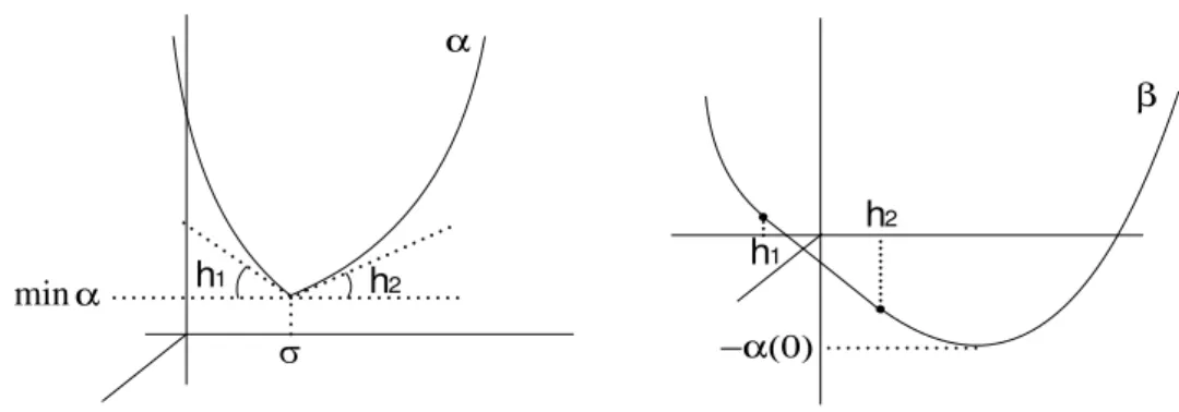
Lemma 3.12 The Ma˜n´e’s critical value of L is α(0) = b(a)2/2, where a ∈ Γmin.
Moreover, the closed curves γa defined by γa(t) = (a,−b(a)t), are static curves.
Proof: Given any curve β(t) = (x(t), y(t)) on T2,we have
L(β,β˙)= x˙
2+ ˙y2
2 +b(x) ˙y(t) =
( ˙y+b(x))2+ ˙x2
2 −
b(x)2 2 ≥ −
b(a)2
2 . (3.2) Then
A
L+b(a2)2 (β) =
∫ T
0
(
L(β,β˙)+b(a)
2
2
)
dt ≥0,
and we obtain α(0) ≤ b(a2)2. Observe that if 0 < k ≤ b(a2)2, the closed curve given by
γk(t) =
(
a,√2kt),wherea ∈Γmin,is Euler-Lagrange solution and its energy isE =k.
Moreover,
AL+k(γk) =
∫ T
0
(L(γk,γ˙k) +k)dt=
∫ T
0
(
2k+b(a)√2k)dt.
Therefore
AL+k(γk)<0 if k <
b(a)2
2 and AL+k(γk) = 0 if k =
b(a)2 2 .
This shows that α(0) = b(a2)2 and the curve γa is semistatic, i.e. realizes the action
potential. Since γa is a semistatic closed curve, it is static curve.
To complete the example, it suffices to show that the map Ψ : Γmin → AM,
given by Ψ (a) = [(a,0)], where [(a,0)] is the static class containing the curve γa, is a
Lipschitz bijection. In fact, since the action potential ΦL+α(0) is Lipschitz, the distance
δM on quotient Aubry set AM is also Lipschitz.
In order to show the surjectivity of Ψ it is enough to show that the projected Aubry set A0 is exactly the union of the closed curves γa witha ∈Γmin. Suppose that
there exists p ∈ A0 such that π(p) ∈/ Γmin, where π is the canonical projection on
the first coordinate ofT2 on R/Z. Then there exists a neighborhood Vp of psuch that
b(x) > b(a) for all a ∈ Γmin and x ∈ Vp. Let γ be a piece, contained in Vp, of the
static curve passing throughp. The inequality (3.2) impliesAL+α(0)(γ)>0.Moreover,
it follows by inequality (3.2) which the actionL+α(0) of any curve is nonnegative, so ΦL+α(0)(x, y)≥0 for all x, y ∈T2. Then
AL+α(0)(γ) = ΦL+α(0)(γ(0), γ(T)) =−ΦL+α(0)(γ(0), γ(T))≤0.
31 Chapter 3. A generic property of exact magnetic Lagrangians
If Ψ is not injective there existsu ∈Γmin, σ̸=a such that (u,0)∈[(a,0)]. Since
each static class is connected (See G. Contreras and G. Paternain in [10], Proposition 3.4) andu∈π([(a,0)]) we have thatπ([(a,0)])⊂R/Zis connected so it is an interval. By total disconnectedness of Γmin, there existsq ∈π([(a,0)])−Γmin.The contradiction
follows of the inequality (3.2) by same above argument.
3.5
Questions
In this section we present some questions still unanswered:
Problem 3.13 The Kupka-Smale Theorem for exact magnetic Lagrangians may be generalized for manifolds of dimension>2?In others words, the property: Any periodic orbit in the level is nondegenerate and all heteroclinic intersections, in this level, are transversal, is generic in the set of exact magnetic Lagrangians?
Problem 3.14 Let L an exact magnetic Lagrangian on the flat torus T2. Then there are no minimizing ergodic measures with homology h= 0.
Problem 3.15 Let M be a closed surface andL an exact magnetic Lagrangian. Then there exists a residual subset O0 of Γ1(M) such that for any ω ∈ O0, the set V (ω) of
cohomology classes csuch that the Aubry set Aec(L+ω) is a finite union of hyperbolic
Chapter 4
A dynamical condition for
differentiability of Mather’s average
action
In this chapter we reproduce the preprint A dynamical condition for differentia-bility of Mather’s average action (see [29]). We are interested in the following question: what can we say about the differentiability ofβ at homologieshsuch that the invariant measures with vector rotation h are supported on an invariant Lipschitz Lagrangian graph?
In this work we give a dynamical condition in order to answer to this question. We obtain differentiability of β in these homologies if the invariant graph is an absorbing graph, i.e. a graph which does not contain ω-limit of minimizing curves out of it.
In Section 4.7 we present a weaker condition for integrability in the case of the torus T2 in order to obtain invariant Lipschitz Lagrangian graphs.
4.1
Aubry and Ma˜
n´
e sets and Hamilton-Jacobi
equa-tion
Given a cohomology class cand a closed 1-form ηc with [ηc] = c, we consider the
Hamilton-Jacobi equation
H(x, ηc(x) +dxu) =α(c). (HJ)
33 Chapter 4. A dynamical condition for differentiability of Mather’s average action
A Lipschitz function u : M → R is called a subsolution of Hamilton-Jacobi for the Lagrangian L−cif, for some closed 1-form ηc with [ηc] = c, we have
H(x, ηc(x) +dxu)≤α(c), (4.1)
at almost every point. Note that this definition is equivalent to the notion of viscosity subsolutions (see [14]). We denote by C1,1 the set of differentiable functions with
Lipschitz differential. Observe that a C1,1 function u is solution of (HJ) if and only if
the graph of ηc+du,denoted by Gηc,u,is invariant under the Hamiltonian flow.
We now recall the definition of calibrated curves (see [14]). If u : M → R is a subsolution of Hamilton-Jacobi for L −c, we say that the curve γ : I → M is (u, L−c, α(c))-calibrated if, for the representative ηc of the cohomology class c given
in (4.1), we have the equality
u(γ(t))−u(γ(t′)) =
∫ t t′
L(γ(s),γ˙ (s))−ηc( ˙γ(s)) +α(c)ds,
for all t′, t∈I. The subset Ie
c(u) ofT M is defined by
e
Ic(u) =
{
(x, v)∈T M :γ(x,v) is (u, L−c, α(c)) -calibrated
}
,
where γ(x,v) =π◦φtL(x, v). The set Iec(u) is invariant and the curves contained in it
are called c-minimizing curves.
By using the sets Iec(u), one can give (see [15]) the following characterization of
the Ma˜n´e set and of the Aubry set contained in T M:
e
Nc =
∪
u∈SSc
e
Ic(u) and Aec =
∩
u∈SSc
e
Ic(u),
where SSc is the set of subsolution of (HJ) for L−c. These invariant sets contain
the Mather set and have interesting dynamical properties, for instanceAec also is graph
whose projection is laminated by global minimizers and it is chain recurrent. The Ma˜n´e setNec is connected and chain transitive (see for instance [9]).
By using the duality between Lagrangian and Hamiltonian, via Legendre trans-form, we define the sets of Mather, Aubry and Ma˜n´e in the cotangent bundle, respec-tively by
M∗c =L
( f
Mc
)
,A∗c =L(Aec
)
e Nc∗ =L(Nec
)
.
Let us denote the projected of Mather, Aubry and Ma˜n´e sets contained in M, respectively by Mc,Ac and Nc.
Remark 4.1 One useful way to produce invariant Lipschitz Lagrangian graphs is to show that Ac = M. If this is the case, Theorem 2.5 of [15] says that there exists an
unique solution u of (HJ) for the Lagrangian L−c which is C1,1 and such that A∗
c is
4.2. Absorbing sets 34
4.2
Absorbing sets
Ifu: M →R is a subsolution of (HJ) forL−c, we denote by Ie+
c (u) the subset
of T M defined as
e
I+
c (u) =
{
(x, v) :γ(x,v)|[0,+∞) is (u, L−c, α(c)) -calibrated
}
,
where γ(x,v) is the curve defined onR by
γ(x,v)(t) =π◦φLt (x, v).
The forward Ma˜ne set is defined by
e
N+
c =
∪
u∈SSc
e
I+
c (u),
where SSc is the set of critical subsolutions for the Lagrangian L−c. We define the
forward tiered Ma˜n´e set as the union of all forward Ma˜ne sets, i.e. the subset ofT M
given by
NT
+ (L) =
∪
c∈H1(M)
e
Nc+.
Definition 4.2 We say that an invariant set Λ ⊂ T M is an absorbing set if for all (x, v)∈ NT
+ (L) we have
ω(x, v)⊂Λ⇒(x, v)∈Λ
Definition 4.3 LetG ⊂T∗M be an invariant Lipschitz Lagrangian graph. We say that
G is an absorbing graph if L−1(G) is an absorbing set.
Lemma 4.4 If (x, v)∈Ne+
c , then the ω-limit set ω(x, v) is contained inAec.
Proof: In fact, let (x, v) ∈ Ne+
c and γ : R → M the projection of Euler-Lagrange
solution γ(t) = π◦φL
t (x, v) curve such that γ|[0,+∞) is (u, L−c, α(c))-calibrated for
some u∈ SSc. This means that there exists a closed 1-form ηc with [ηc] =csuch that
H(x, ηc(x) +dxu)≤α(c) at almost every point and
u(γ(t))−u(γ(t′)) = AL−ηc+α(c)
(
γ|[t′,t]
)
for all 0< t′ < t.
Let (y, z)∈ω(x, v), i.e. (y, z) = limn→∞(γ,γ˙) (tn) with tn → ∞.
Let us considerσ :R→M the projection of the Euler-Lagrange solution σ(t) =
π◦φL
35 Chapter 4. A dynamical condition for differentiability of Mather’s average action
exists a closed 1-form ξc with [ξc] = c and H(x, ξc(x) +dxu) ≤α(c) at almost every
point. It follows from ([14], Proposition 4.2.3) that u satisfies
u(γ(t))−u(γ(t′))≤AL−ξc+α(c)
(
γ|[t′,t]
)
,∀t′ < t.
We can consider V ∈ C∞(M) a function such that η
c = ξc +dV. Thus, if s > 0 and
(tk) and (tm) are two subsequences of (tn) such thattk−s > tm+s and tk, tm > s,we
have
AL−ξc+α(c)
(
σ|[−s,s]
)
+u(σ(−s))−u(σ(s)) = lim
m,k
[
AL−ξc+α(c)
(
γ|[tm−s,tm+s]
)
+u(γ(tk−s))−u(γ(tm+s))
]
≤lim
m,k
[
AL−ξc+α(c)
(
γ|[tm−s,tm+s]
)
+AL−ξc+α(c)
(
γ|[tm+s,tk−s]
)]
= lim
m,kAL−ξc+α(c)
(
γ|[tm−s,tk−s]
)
= lim
m,k
[
AL−ξc−dV+α(c)
(
γ|[tm−s,tk−s]
)
+V (γ(tk−s))−V (γ(tm−s))
]
= lim
m,kAL−ηc+α(c)
(
γ|[tm−s,tk−s]
)
+V (γ(−s))−V (γ(−s)) = lim
m,ku(γ(tk−s))−u(γ(tm−s))
=u(γ(−s))−u(γ(−s)) = 0.
Therefore
AL−ξc+α(c)
(
σ|[−s,s])≤u(σ(s))−u(σ(−s)).
The opposite inequality holds because u is a Hamilton-Jacobi subsolution (see [14], Proposition 4.2.3). This shows that
(y, z)∈ ∩
u∈SSc
e
Ic(u) =Aec.
Examples of absorbing graphs are the so-called Schwartzman strictly ergodic graphs (see [16], Definition 2.4):
Definition 4.5 A Lagrangian graph Λ is called Schwartzman strictly ergodic graph if there exists an invariant measure with full support.
Let us to show that an Schwartzman strictly ergodic graph Λ is an absorbing graph. Indeed, let µ be the invariant measure supported on Λ with ρ(µ) = h. Let us consider ω(x, p) ⊂ Λ for some (x, p) ∈ L(NT
+ (L)
)
4.2. Absorbing sets 36
L(Ne+
c
)
for some cohomology class c. It follows from above lemma that ω(x, p) ⊂ A∗
c ∩Λ.Since Λ =L
( f
Mh), we have
ω(x, p)⊂ L(Mfh)∩ A∗c.
This shows thatL(Mfh)∩ A∗
c ̸=∅ and supp(µ)⊂ M∗c. Moreover, sinceπ(supp(µ)) =
M, we obtainA∗
c = Λ. By the graph property, we conclude that (x, p)∈Λ.
Actually, the same argument can be used to prove that an invariant graph Λ such that all invariant probability measures with support contained in Λ have the same rotation vector h and the union of their supports equals Λ is also absorbing.
Proposition 4.6 Let Λ ⊂ T M be an invariant absorbing set. If Aec ⊂ Λ for some
c∈H1(M;R), then Λ projects onto the whole manifold M.
Proof: Let us consider a closed 1-form ηc representative of the cohomology class c. It
follows from ([14], Theorem 4.9.3) that there exists a weak KAM of positive type u+
for the LagrangianL−ηc. Thenu+ is subsolution of (HJ) and givenx∈M we can find
a C1 curve γ
x : [0,∞) → M with γx(0) = x, which is (u+, L−ηc, α(c))-calibrated.
This means that for all 0< t′ < t holds
u+(γx(t))−u+(γx(t′)) =
∫ t t′
L(γx(s),γ˙x(s))−ηc( ˙γx(s)) +α(c)ds.
Therefore (γx,γ˙x) ∈ Iec+(u+)⊂ Nec+ and, by Lemma 4.4, we have that the ω-limit set
of (γx,γ˙x) is contained in Aubry setAec. Since Λ is an absorbing set that contains Aec,
we obtain (x,γ˙x(0))∈Λ.
Lemma 4.7 Let c∈H1(M;R) and h∈ H
1(M;R). We have Mfh ⊂Mfc if and only
if c∈∂β(h).
Proof: If Mfh ⊂Mf
c, then there exists a c-minimizing measure µ with ρ(µ) = h. So
−α(c) =
∫
T M
(L−ηc)dµ=
∫
T M
Ldµ− ⟨c, h⟩=β(h)− ⟨c, h⟩,
where ηc is a representative of the cohomology classc. This shows that c∈∂β(h).
Conversely, letµminimizing measure with rotation vector h. If c∈∂β(h), then
β(h) =⟨c, h⟩ −α(c). Therefore
−α(c) =β(h)− ⟨c, h⟩=
∫
T M
Ldµ− ⟨c, ρ(µ)⟩=
∫
T M
(L−ηc)dµ.