ESTRUTURA DE COVARIÂNCIA EM MODELOS
BAYESIANOS ESPACIAIS
ESTRUTURA DE COVARIÂNCIA EM MODELOS
BAYESIANOS ESPACIAIS
Tese apresentada ao Programa de Pós-Graduação em Estatística da Universidade Federal de Minas Gerais como requisito parcial para a obtenção do grau de Doutor em Estatís-tica.
ERICA CASTILHO RODRIGUES
ESTRUTURA DE COVARIÂNCIA EM MODELOS
BAYESIANOS ESPACIAIS
Thesis presented to the Graduate Program in Estatística of the Universidade Federal de Mi-nas Gerais in partial fulfillment of the require-ments for the degree of Doctor in Estatística.
ERICA CASTILHO RODRIGUES
FOLHA DE APROVAÇÃO
Estrutura de Covariância em Modelos Bayesianos Espaciais
ERICA CASTILHO RODRIGUES
Tese defendida e aprovada pela banca examinadora constituída por:
Ph. D.Renato Martins Assunção – Orientador Universidade Federal de Minas Gerais
Ph. D.Rosângela Helena Loschi Universidade Federal de Minas Gerais
Ph. D. Marcos Oliveira Prates Universidade Federal de Minas Gerais
Ph. D.Alexandre Loureiros Rodrigues Universidade Federal do Espírito Santo
Ph. D.Thaís Cristina Oliveira da Fonseca Universidade Federal do Rio de Janeiro
Agradeço primeiramente a Deus, por me permitir terminar mais essa etapa.
Não poderia deixar de agradecer em primeiro lugar aos meus pais, Ricardo e Marcia. À minha mãe, pela paciência em me ouvir todos os dias, por participar em todos os momento, sempre me confortando e me incentivando. Ao meu pai, por sempre acreditar em mim, por sempre me ajudar em tudo que fosse possível. À Gabriela, pela compreensão e pela torcida sempre constante. Gostaria de agradecer também ao Taciano, pelo amor e incentivo incondicionais. Por sempre me ouvir, me dar conselhos e por sempre compartilhar comigo cada momento dessa jornada. Não poderia deixar de agradecer também a todos de sua família, Mariana, Arnaldo, Huascar e Glenda, muito obrigada por tudo. Agradeço às minhas grandes amigas, Poliana, Natália e Sarah, pelos ótimos momentos compartilhados e por sempre torcerem por mim.
Devo agradecer também a todos os amigos da UFMG. À Vanessa, com seu jeito meigo e generoso, quantos momentos de sufoco não passamos juntas. Às meninas do Leste, Aline, Letícia, Thaís, Márcia, Paola pelas horas de trabalho tão agradáveis ao lado de vocês. Pelos muitos momentos de descontração e por fazerem meu dia bem mais divertido. Ao João Vitor, pelo pouco tempo que trabalhamos juntos. Ao Marquinhos por toda a ajuda acadêmica e pelo bom humor a todo momento. Gostaria também de agradecer a todos os mestres do Departamento de Estatística. Em especial à Rosângela e Denise, pelo incentivo sempre e pelo tanto que me ensinaram. Não posso deixar de agradecer também aos mestres do Departamento de Matemática, Bernardo e Remy, que acreditaram em mim bem no comecinho e me iniciaram na vida acadêmica. Gostaria também de agradecer ao Renato pela orientação, sempre firme, segura, por me mostrar com é importante amar o que se faz. Pela paciência em entender minhas dificuldades e por me motivar a superá-las a todo momento. Gostaria de agradecer também aos professores Alexandre Loureiros, Marcos Oliveira, Thaís Fonseca e Wagner Meira pelos comentários valiosos para melhoria deste trabalho.
No mapeamento de doenças, é necessário especificar uma estrutura de vizinhança para fazer inferências sobre a distribuição geográfica dos riscos relativos. Essa estrutura pode ser usada para modelar a dependência espacial dos dados. Um ponto importante é como modelar essa dependência, qual tipo de covariância será definida entre os pares de áreas. Neste trabalho é feita uma análise da estrutura de covariâncias para dados de áreas. Em partes desse trabalho novos modelos são propostos e, em outras, modelos presentes na literatura são analisados cuidadosamente. Em um contexto um pouco diferente, a dependência entre os dados pode ser utilizada para recuperar outros tipos de informação, como, por exemplo, a localização dos eventos. Resolvemos esse tipo de problema para o caso específico de uma rede social, o Twitter. As arestas do grafo agora não representam mais vizinhança geográfica, mas sim relações de amizades entre os usuários. Mostramos como essa informação associada ao tipo de publicação de cada usuário pode ser utilizada para inferir sua localização.
Palavras-chaves: Mapeamento de doenças; Campos Aleatórios de Markov; Modelos Hierárquicos Espaciais; Naive Bayes; Twitter.
In disease mapping, one must specify a neighborhood structure to make inferences about the geographic distribution of the relative risks. This structure can be used for modeling spatial dependence of the data. An important point is how to model this dependence, which type of covariance is defined between pairs of areas. This work presents an analysis of covariance structure for area data. In parts of this work new models are proposed and in other parts some models proposed in the literature are analyzed carefully. In a somewhat different con-text, the dependency between data can be used to retrieve other kind of information, such as the location of events. We solve this kind of problem for the specific case of a social network,
Twitter. The edges of the graph no longer represent geographical neighborhood, but friend-ships relationfriend-ships among users. We show how this type of information associated with the publication of each user can be used to infer their location.
Key words: Disease Mapping ; Markov Random Fields, Hierarchical Spatial Models; Naive Bayes; Twitter.
O mapeamento das taxas de doenças é de grande importância em estudos de epidemiologia. Essa técnica permite analizar como determinada doença se espalha na região em estudo, levando em conta características ambientais, socio-econômicas, genéticas e fatores como o risco de contágio. Dessa maneira, torna possível a identificação de locais com risco elevado e que, portanto, devem sofrer intervenção por agentes de saúde. Elliott e Wartenberg (2004) [26] fazem uma revisão sobre o assunto, apresentam alguns problemas relacionados a esse tipo de análise, bem como técnincas que vem sendo desenvolvidas.
O procedimento que é adotado usualmente consiste em mapear o estimador de máxima verossimilhança dessa quantidade, que é denominado SMR (Standardized Mortality Ratio), sobre as diferentes regiões geográficas. Esse estimador é dado pela razão entre o número de casos da doença observados naquela área, pelo número que seria esperado caso não houvesse nenhuma estrutura espacial, ou seja, se o número de casos dependesse apenas da população sob risco.
Porém, quando a doença é rara e a população é muito pequena, essas estimativas são muito instáveis e acabam causando distorções na apresentação do mapa. Isso torna inviável a visualização de padrões de distribuição da doença. A solução encontrada para esse prob-lema é tentar suavizar essa estimativa. Essa suavização pode ser feita utilizando-se Modelos Bayesianos Hierárquicos. Nesse tipo de modelagem, supõe-se que as contagens da doença seguem uma distribuição de Poisson com uma média que é igual ao risco relativo da área multiplicado pelo número de casos esperados na região sob a hipótese de risco constante. O logaritmo do risco relativo é modelado por uma normal cuja média pode depender de algumas covariáveis e soma-se a essa média um erro aleatório que apresenta uma estrutura espacial. Isso é feito colocando uma distribuição a priori que reflita tal variabilidade. Essa estrutura deve comportar aspectos que são semelhantes entre áreas próximas no mapa, como caracterís-ticas ambientais, econômicas e sociais. Tais distribuições a priori podem ser definidas como Campos Markovianos. Isso siginifica que a distribuição condicional de uma área dadas as suas vizinhas não depende do resto do mapa. Em outras palavras, áreas que não são vizinhas são condicionalmente independentes. No caso em que as variáveis aleatórias têm distribuição normal, essa estrutura de indepedência condicional é definida através da inversa da matriz de precisão, ou seja, a inversa da matriz de covariâncias da distribuição normal multivariada. Esses tipos de modelos são conhecidos como Campos Markovianos Gaussianos e um detalhado estudo sobre esse assunto pode ser encontrado em Rue et at. (2005) [63]. Os termos não nulos
importante é a especificação da estrutura de vizinhança. Essa estrutura é responsável por induzir certos tipos de relação de dependência entre as áreas.
Neste trabalho analisamos esse tipo de dependência em determinados contextos e verifi-camos como ela se comporta para alguns modelos específicos. Apresentamos uma maneira alternativa de se definir a estrutura de vizinhança espacial e mostramos quais as consequências dessa definição para a matriz de covariâncias induzida. Mostramos ainda que determinados tipos de modelos podem apresentar interpretações até o momento não evidentes, mas que podem ajudar na análise de resultados em aplicações práticas. Analisamos ainda casos em que a definição desse tipo de modelo leva a resultados não intuitivos que devem ser analisados com cuidado para evitar que modelos sem sentido prático sejam ajustados a diversas bases de dados sem muita cautela.
Lidamos ainda com um tipo de problema em que a variável para a qual se deseja se fazer inferência é a própria localização. Apenas parte da base de dados possui essa informação disponível e queremos realizar uma imputação para os casos em que ela não está presente. Essa imputação é feita considerando a estrutura de dependência entre os dados, que é modelada utilizando-se um grafo. Mais uma vez, um ponto importante é como incorporar no modelo essa dependência entre os dados e utilizar essa informação de maneira adequada para realizarmos nossas estimações. Uma complicação adicional neste segundo tipo de problema é o grande volume de dados que estamos tratando. Os dados se referem a usuários de redes sociais, o que significa que o número de nós do grafo possui uma ordem de grandeza muito superior àquela quando estamos trabalhando com mapeamento de doenças. Dessa maneira, os métodos propostos devem ser simples o suficiente a fim de não tornar o processo inferencial inviável computacionalmente.
Neste trabalho apresentamos soluções para os problemas acima descritos e mostramos através de resultados práticos e teóricos quais as vantagens e os pontos fracos das metodolo-gias propostas. O texto está dividido em quatro artigos independentes entre si que serão brevemente descritos a seguir.
O primeiro deles é intitulado Bayesian spatial models with a mixture neighborhood struc-ture e foi publicado em Agosto de 2012 no Journal of Multivariate Analysis. Nesse artigo apresentamos um modelo para dados espaciais no qual a estrutura de vizinhança é parte do espaço paramétrico. Mantemos a propriedade markoviana dos modelos Bayesianos espaciais: dado o grafo de vizinhança, a taxa de incidência de uma doença segue um modelo condicional autoregressivo. Definimos a matriz de precisão do modelo de uma maneira mais flexível. Isso permite que o modelo seja capaz de ajustar diversos tipos de estruturas espaciais presentes nos dados. Analisamos as propriedades teóricas do modelo proposto e mostramos que ele apresenta resultados superiores aos demais tanto para casos simulados como para exemplos reais.
O segundo artigo, Covariance decomposition in multivariate spatial models, consiste em uma análise cuidadosa de um modelo espacial para dados multivariados. Nesse caso, a resposta
cada área e a depenência entre variáveis observadas em áreas distintas. Esse modelo é definido a partir de um conjunto de distribuições condicionais que apresentam um formato intuitivo. Porém as covariâncias marginais induzidas apresentam um formato complexo. Para fins de interpretação de modelos ajustados, é de grande importância entendermos como as correlações marginais se comportam. Nós mostramos neste trabalho que as matrizes de covariâncias a priori e a posteriori podem ser escritas como uma soma infinita de matrizes. Obtemos interpretações para as componentes que aparecem nessa soma e mostramos através de um exemplo real como tais interpretações podem auxiliar na análise de problemas práticos.
O terceiro artigo, cujo título é Analisando o modelo espacial de decaimento exponencial, consiste em uma análise de um modelo espacial econométrico. Esse modelo foi proposto por [49] e consiste em uma tentativa de resolver problemas numéricos adjacentes ao processo de inferência de modelos espaciais para dados de área. Apesar de tornar o processo inferencial mais eficiente computacionalmente, esse modelo possui uma estrutura de correlações marginais pouco intuitiva. Mostramos que ele apresenta comportamentos não intuitivos para diversos tipos de grafos de vizinhança, desde os mais simples até os mais complexos. Em especial, mostramos que para esse modelo podemos ter situações em que as correlações marginal e condicional entre duas áreas podem ter sinais opostos. Esse tipo de comportamento não é observado para modelos clássicos de séries temporais, como os modelos Autoregressivos, e nem para modelos bastante difundidos em estatística espacial, como os Condicionais Autore-gressivos. Mostramos esses resultados através de exemplos experimentais e demonstrações analíticas.
No quarto artigo, Inferindo a localização de usuários do Twitter, analisamos um outro tipo de dado. Nosso grafo agora é formado por relações de amizades entre usuários de redes sociais, em particular do Twitter. O nosso objetivo nesse caso é inferir a localização dos usuários. Alguns trabalhos apresentados na literatura, como Davis et al. (2004) [24], utilizam a rede de amizades para fazer essa inferência. Outros trabalhos , como de Cheng et al. (2012) [19], coletam informação do texto para alcançar esse objetivo. Vamos incorporar as duas informações e usá-las simultâneamente para fazer inferência sobre a localização. Essa inferência é feita a nível de cidade. Portanto vamos atribuir um rótulo a cada usuário do grafo, que corresponde à cidade na qual ele mora. Consideramos que esse rótulos dispostos no grafo seguem um Campo Markoviano. Nesse caso, como a variável resposta é categórica, não é viável utilizar um Campo Gaussiano. Utilizamos, então, o Modelo de Potts que é muito utilizado na área de processamento de imagem e consiste em um Campo Markoviano para o qual a variável resposta corresponde a uma classificação dos sítios. Nesse modelo, a suposição principal é de que áreas conectadas diretamente tenderão a pertencer à mesma classe. Para recuperarmos a informação do texto utilizaremos o método Naive Bayes. Esse método classifica objetos com base em um conjunto de caracteríticas. No nosso casso, esse conjunto de características são as palavras postadas pelos usuários. Uma suposição subjacente ao método é de que, dadas as classes dos objetos, tais características são independentes entre si. Unindo essas
metodologia proposta atinge taxas de acertos muito superiores aos trabalhos apresentados na literatura.
1 Bayesian spatial models with mixture neighborhood structure 1
1.1 Introduction . . . 1
1.2 Disease Mapping . . . 3
1.3 Model definition . . . 5
1.4 Model properties . . . 8
1.5 Posterior Covariance Matrix . . . 12
1.5.1 The special case of two components . . . 14
1.6 Illustrative application . . . 14
1.6.1 Including covariates . . . 17
1.7 Simulation study . . . 18
1.8 Conclusions . . . 22
2 Covariance decomposition in multivariate spatial models 23 2.1 Introduction . . . 23
2.2 Model Definition . . . 25
2.3 Covariance matrix . . . 28
2.3.1 Blocking by areas . . . 29
2.3.2 Blocking by variables . . . 32
2.4 Interpreting the decomposition . . . 32
2.5 Posterior Covariance Matrix . . . 35
2.6 An illustrative synthetic example . . . 37
2.7 Concluding remarks . . . 40
3 Analisando o modelo espacial de decaimento exponencial 42 3.1 Introdução . . . 42
3.2 Definição do Modelo . . . 44
3.3 Lattice Regular . . . 46
3.4 Lattice unidimensional . . . 48
3.5 Lattice irregular espacial . . . 51
3.5.1 Como a correlação parcial varia comα . . . 55
3.6 Conclusão . . . 58
4 Inferindo a localização de usuários do Twitter 59
4.3 Metodologia . . . 65 4.4 Resultados Experimentais . . . 66 4.5 Conclusão . . . 69
Bibliography 70
1.1 QQ-plot of p-values using Gamma(0.5, 0.0005) for all components, three compo-nents, Leroux and Bym models. The p-values were calculated using the cross-validation proposal of [57]. . . 18 1.2 QQ-plot of p-values using Gamma(0.01, 0.01) for all components, three
compo-nents, Leroux and Bym models. The p-values were calculated using the cross-validation proposal of [57]. . . 19 1.3 Posterior density of theβ coefficients for three covariates using our model with all
components for the spatial random effect. The first plot refers to the proportion of Black and American Indians in the population, the second plot refers to proportion of mothers who had prenatal care and the third plot refers to the proportion of mothers who were smokers. . . 20
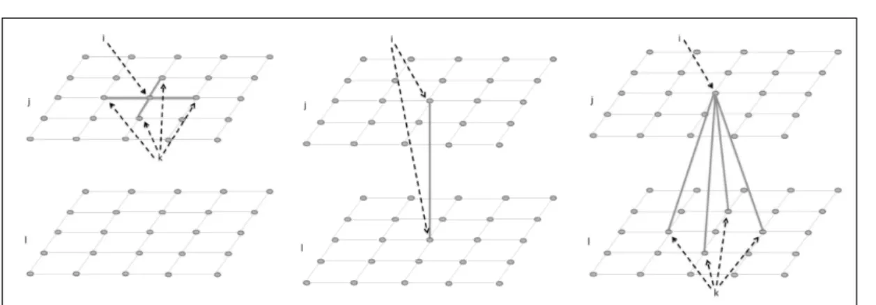
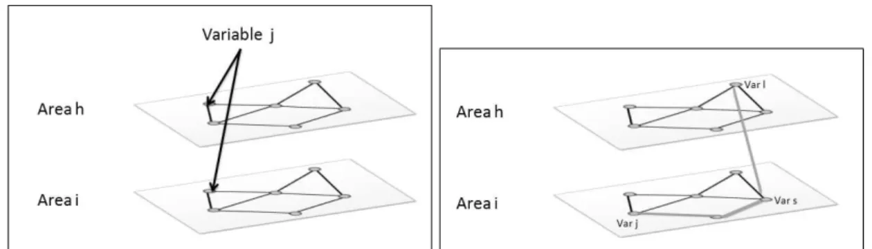
2.1 Examples of different types of neighborhoods using variables j and l measured in a spatial regular lattice. The left hand side frame shows a within-variable spa-tial neighborhood, while the middle frame shows a within-location neighborhood. The right hand side frame demonstrates the neighborhood associated with cross-variable connections. . . 27 2.2 Dual graph of areasiand k(right). An example of a possible path between these
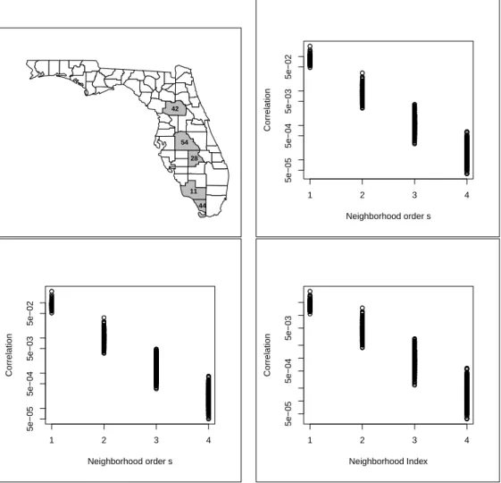
areas (left). . . 34 2.3 Map of Florida counties with some areas identified. The other three plots show the
marginal correlations Cor(Yij, Ykl) (in log-scale) versus the spatial neighborhood
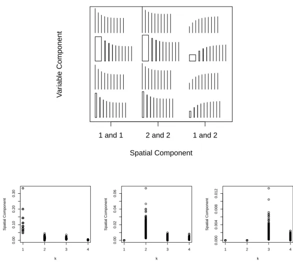
orders. In clockwise direction, they represent variables(j, l)equal to(1,1),(2,2), and (1,2). . . 38 2.4 Top: Rectangles showing the spatial and variable components of covariance
be-tween Yij and Ykl for increasing neighborhood order k and for different pairs of
areas. Bottom: Spatial component as a function ofkfor all first, second, and third order spatial neighboring areas. . . 39
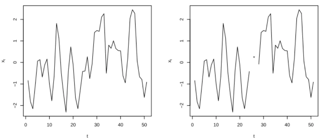
3.1 Série temporal com 51 observações simuladas (esquerda) e série simulada retirando-se as obretirando-servações de ordem 25 e 27 (direita). . . 49
cionais (esquerda). Gráfico de dispersão das cinco observações geradas a partir da
distribuição condicional (direita). . . 50
3.3 Série temporal gerada, linhas tracejadas representam as 20 observações geradas a partir das distribuições condicionais e os pontos marcam as esperanças condi-cionais (esquerda). Gráfico de dispersão das 200 observações geradas a partir da distribuição condicional (direita). . . 50
3.4 Série temporal gerada de um processo autoregressivo de ordem 2. Linhas tracejadas representam as 20 observações geradas a partir das distribuições condicionais e os pontos marcam as esperanças condicionais (esquerda). Gráfico de dispersão das 200 observações geradas a partir da distribuição condicional (direita). . . 51
3.5 Mapa Iowa representando correlações marginais e condicionais entre pares de áreas vizinhas. A primeira figura mostra o mapa de Iowa com as ligações representando vizinhos de primeira ordem. A segunda mostra ligações entre vizinhos de primeira ordem que possuem correlação marginal positiva. A terceira figura mostra lig-ações entre pares de áreas vizinhas que possuem correlação condicional positiva. A quarta figura mostra ligações entre pares de áreas que possuem correlações condicionais negativas. . . 52
3.6 Vizinhos de primeira ordem, vizinhos de primeia ordem com correlação marginal positiva, vizinhos de primeira ordem com correlação parcial positiva e vizinhos de primeira ordem com correlação parcial negativa. . . 53
3.7 Vizinhos de segunda ordem, vizinhos de segunda ordem com correlação marginal positiva, vizinhos de segunda ordem com correlação parcial positiva e vizinhos de segunda ordem com correlação parcial negativa. . . 54
3.8 Correlação entre vizinhos de primeira ordem para diferentes valores de α. . . 56
3.9 Correlação entre vizinhos de segunda ordem para diferentes valores de α. . . 57
4.1 Grafo de relações amizades dos 8477 usuários coletados. . . 67
4.2 Matrizes de confusão dos resultados obtidos aplicando-se a metodologia proposta. A matriz à esquerda apresenta medidas de sensibilidade e à direita as medidas de precisão do método. . . 68
1.1 DIC and Logarithm Score criteria for North Carolina data base using Gamma(0.5,0.0005)
(first row) and Gamma(0.01,0.01)(second row). The models compared are BYM, Leroux and our model with all and with three components. The logarithm score criterium is evaluated with the importance weights and the importance resampling methods. . . 16 1.2 M SE,DIC, and LS for the simulation of the six scenarios. Summary statistics
are the average of 10 independent replications of each model. . . 21
Bayesian spatial models with mixture
neighborhood structure
Abstract
In Bayesian disease mapping, one needs to specify a neighborhood structure to make inference about the underlying geographical relative risks. We propose a model in which the neighborhood structure is part of the parameter space. We retain the Markov property of the typical Bayesian spatial models: given the neighborhood graph, disease rates follow a conditional autoregressive model. However, the neighborhood graph itself is a parameter that also needs to be estimated. We investigate the theoretical properties of our model. In particular, we investigate carefully the prior and posterior covariance matrix induced by this random neighborhood structure, providing interpretation for each element of these matrices.
Keywords: Disease mapping; Markov Random Field; Spatial Hierarchical Models.
1.1 Introduction
In disease mapping, the Bayesian model proposed by [12], and denoted by BYM, is the most popular choice to estimate relative risks in small areas or to evaluate the effects of covariates acting as exposure measurements surrogates. Originally, BYM was introduced to model a cross-section of counts collected in a set of disjoint geographical areas composing a partitioned map. Since then, BYM has been extended into several directions to include space-time generalized linear models [52, 58, 43, 71, 67], spatial survival models [17, 39], spatially-varying parameters models [5, 1, 28], and generalized additive models [45]. Multivariate extensions incorporating two correlated sets of spatial effects have also been proposed in recent years [39, 30, 35, 34]. Many of these models can be fit using freely available software such as WinBUGS [51] and BayesX [16].
BYM is based on a conditional autoregressive (CAR) model for the spatial random effects. In the CAR model, spatial dependence is expressed conditionally by requiring that the random effect in a given area, given the values in all other areas, depends only on a small set of
neighboring values. More specifically, the random effectbi associated with thei-th area is the
sum ϕi+θi of two components, where ϕi is a spatially structured random effect assigned an
improper CAR prior distribution andθiis a second set of i.i.d. zero-mean normally distributed
unstructured random effects. This is termed a convolution prior [12] because the density of
bi’s will be the convolution of the joint densities of theϕi andθi vectors.
An essential aspect of the BYM model and its extensions is the specification of the neigh-borhood structure for the areas. Although this is quite flexible and can be arbitrarily defined, in practice it is typically based only on adjacency relationships. There are few justifications for this practice other than its easy calculation by means of GIS (Geographic information system) routines. A related problem with the BYM model is that the neighborhood structure determines the smoothing degree used in relative risk estimation. Some authors noticed its tendency to oversmooth the risks when the usual adjacency neighborhood structure is used. Therefore, it would be very useful to have a model that allows for multiple neighborhood structure and automatically adapts itself according to the observed data.
Despite its crucial role in spatial Bayesian models, very few studies have considered dif-ferent neighborhood structures for disease mapping problems. One notable exception is [52] where the authors considered a model for disease rates with spatial effects structured at two geographical levels. They used infant mortality data over the period 1985-1994 from the province of British Columbia (BC) in Canada. The areas were organized in 21 health units (HUs) that were further subdivided into 79 local health areas (LHAs). Health units (HUs) are administrative health divisions overseeing the functioning of the health sub-units, the local health areas (LHAs). Therefore, it was natural to expect that LHAs within the same HU should share many health service and care characteristics beyond those determined by factors that vary smoothly in space. Hence, they assumed a random effect shared by all LHAs within the same HU. They also considered a neighborhood structure in which two LHAs are considered neighbors if they share boundaries or if there is a third LHA sharing boundaries with both local health areas. This second-order neighborhood structure is less common and it recalls the higher autoregressive order models in the time series setting.
A more recent reference is [74], who introduced a stochastic neighborhood CAR model where the neighborhood selection depends on unknown parameters. They estimate neigh-borhood sizes by assuming that there is an unknown cutoff distance. Within this distance proximity weights are equal and sum to one, and beyond it they decline exponentially with distance, reaching zero at the edge of the map. In contrast with most of published applied pa-pers in disease mapping, they base their model on the proper CAR speficication rather than BYM. Most people prefer to use BYM, implying in an improper CAR model to deal with the spatial random effects, because the proper CAR model induces little marginal correlation between neighboring areas (see [7], page 81) and [2].
either unstructured overdispersion or small-scale spatial conditional variation. These are two extreme models and allowing for intermediate situations will be useful in some applications. We will show examples where the typical adjacency neighborhood structure is not sufficient to estimate the underlying risks, providing less smooth estimates than what should be inferred from the data. Our purpose is to introduce spatial effects with that extend beyond the imme-diate geographical neighborhood. This is likely to be especially useful in situations where the underlying risk changes so smoothly over larger regions as to be considered indistinguishable from a random constant value for all areas within it.
In this work, we investigate more flexible neighborhood structures for spatial conditional autoregressive models. We propose a model in which the neighborhood structure is part of the parameter space. We retain the Markov properties of most Bayesian spatial models. That is, the disease rates follow a conditional autoregressive model, given the neighborhood graph. However, the neighborhood graph itself is a parameter that also needs to be estimated. The methodology described herein permits arbitrary neighborhood extension for incorporating spatial random effects. It provides a simple mechanism for identifying the geographical extent of the conditional influence of neighboring areas.
The manuscript is organized as follows. In Section 1.2, we introduce the notation and present some models that were proposed previously. In section 3.2 present the definition our model. In Section 1.4, we investigate the theoretical properties of the model. In particular, we carefully study the prior and posterior covariance matrix induced by this random neighbor-hood structure, providing interpretation for each element of these matrices. We also present a specific, simple case of our model, allowing for a more thorough understanding of the co-variance structure. In Section 2.6, we illustrate the use of our model for disease mapping. In this section, we also present a simulation study to compare our method with alternative proposals. We end in Section 1.8 with the main conclusions.
1.2 Disease Mapping
A Bayesian hierarchical model is one of the main tools for making inferences about the under-lying relative risks of a disease observed on disjoint geographical areas of a map. Suppose that we have N geographic areas and each has a relative risk ψi for i= 1, ..., N that needs to be
estimated. Bayesian inference is based on the posterior distribution ofψ = (ψ1, ..., ψN)given
by f(ψ|y1, ..., yN) ∝l(y1, ..., yN|ψ)f(ψ), where l(y1, ..., yN|ψ) is the likelihood function and
f(ψ)is the prior distribution of the parameter vectorψ. Conditional on the valuesψ1, ..., ψN,
the values Y1, ..., YN are assumed to be independent with a Poisson distribution with mean
ψiEi, where Ei is the expected value of cases under the hypotheses of constant relative risk
over the areas. Modeling the prior distribution f(ψ) allows the introduction of spatial de-pendence between the risks such that close regions tend to have similar relative risks. This dependence appears as a Markovian structure in which the value ψi of one area, conditional
More specifically, the relative risk ψi is written as
log(ψi) =µ+bi (1.1)
where µ is the general level of the relative risk and bi is the random effect for the i-th
area. One simple possibility is to assume that the random effects bi are independent and
identically distributed with a normal distribution N(0, σ2). In this case, there will be no
spatial effects imposed on the relative risks and the posterior distribution ofψwill reflect this independence. However, one typically expects spatial dependence between the relative risks due to environmental and genetic similarities between neighboring areas. The most popular prior distribution for modeling spatial structure was introduced by [12]. They decomposed the random effect bi into two parts, a non-spatially structured component and a spatially
structured component:
log(ψi) =µ+θi+ϕi
where θ1, . . . , θn are the non-structured errors, independently and identically distributed
ac-cording to a normal distribution. The random effects ϕi have a spatially structured prior
distribution with intrinsic CAR (ICAR) distribution. The ICAR prior distribution is an im-proper prior with a Markovian structure. The distribution of ϕi, conditional on all the other
values ϕj forj ̸=i, is given by
ϕi|φ−i∼N (
¯
ϕi,
σ2 ni
)
(1.2)
whereϕ¯i is the mean of thei-th area neighboring valuesϕj.
This model presents some identifiability problems for the spatial and non-spatial effects, as noticed by [25]. To fix these problem, [47] presented an alternative, including a parameter
λwhich is able to measure the effect of each component. This parameter measures the level of spatial correlation among the areas. In addition to this, it includes a parameterσ2 to measure the random effect variance. They proposed a multivariate normal distribution for the random effects b= (b1, . . . , bN) in (1.1) with the following precision matrix
Q= (σ2)−1((1−λ)I+λR) (1.3)
whereIis the identity matrix andRis the precision matrix of the ICAR model, which means thatRij is equal toni,−1, and0, if i=j,i∼j, and otherwise, respectively, where ni is the
number of neighbors of site iandi∼jmeans ineighbor ofj. For this model, the parameter
λ assumes values in the interval [0,1], so that, the precision matrix Q is a weighted sum of theI and Rmatrices.
about the random effects. We think that in many practical situations this is too restrictive. Consider, for example, another extreme but possible situation in which the distribution of bi
(and hence, ofψi) in a given area, conditional on the rest of the map, should depend upon all
the other sites, not only on the immediate neighbors. In this case, all areas are neighboring areas of all other areas. This can be a reasonable model when the region under study is small enough such that economic, social and environmental characteristics are approximately con-stant over the entire region. This implies on exchangeability between the areas and therefore an all-inclusive dependence between the areas’ pairs. Every area gives incremental additional information on a fixed area value, even if conditioning on all the other areas.
1.3 Model definition
We propose a model that expands the BYM and Leroux models beyond single-neighbor de-pendence of BYM and Leroux models to a larger class that has geographically increasing orders of neighborhood extension. Through Bayesian updating, we can make inference about the more appropriate neighborhood structure underlying the observed data. More specifi-cally, we extend the weighted sum precision matrix (1.3) by including matrices that represent neighborhoods of all possible orders in the simple adjacency graph.
Let each area i be a node or site of a graph and connect two nodes by one edge if they share boundaries. Let A be the n×nbinary adjacency matrix where Aij = 1if i andj are
connected by one edge, and Aij = 0otherwise. We say that area iis an l-th order neighbor
of area j if the (i, j)-th element of the power matrix Al is greater than zero andAsij = 0, for
s < l and l ≥ 1. The maximum neighborhood order is given by the diameter of the graph, which is the longest path among all the shortest paths that connect two sites. In other words, the diameter counts the minimum number of steps necessary to leave a site and go to any other site in the graph.
In our model, the vectorb = (b1, . . . , bN) in (1.1) has a multivariate normal distribution
with mean zero and precision matrix given by:
Q= (σ2)−1(λ1I+λ2R(1)+λ3R(2)+....+λk+1R(k)
)
whereλ1+λ2+...+λk+1 = 1andλi ≥0for alli. The integerkis the diameter of the graph
and R(l) is the graph Laplacian that includes neighborhoods up to order l. That is,
R(ijl) =
n(il) if i=j
−1 ifj ∈∂i(l)
0 otherwise
This matrix is positive definite if λ1 > 0, as it satisfies the sufficient condition of being
diagonally dominant. That is, for all i= 1, . . . , n, we haveQii>∑Nj=1|Qij|because
Qii=λ1+λ2n(2)i +λ3ni(3)+...+λk+1n(ik)=λ1+
N ∑
j=1
|Qij|> N ∑
j=1
|Qij|.
From the precision matrix, it is possible to obtain the conditional distribution bi|b−i of
each area given the vector b−i = (b1, . . . , bi−1, bi+1, . . . , bn). It is a normal distribution with
mean f(b, λ) and varianceg(b, λ) given by
f(b, λ) = λ2n
(1)
i ¯b
(1)
i +λ3n(2)i ¯b
(2)
i +. . .+λk+1n(ik)¯b
(k)
i
λ1+λ2n(1)i +λ3n(2)i +...+λk+1n(ik)
and
g(b, λ) = σ
2
λ1+λ2n(1)i +λ3n(2)i +...+λk+1n(ik)
where ¯b(l)
i is the mean of neighbors of site i up to order l. The conditional expectation
is a convex linear combination of the means of its neighbors of all possible orders and the conditional variance is inversely proportional to the number of neighbors of each of these orders multiplied by their respective weight λl.
Letb−ij be the (n−2)-dimensional vector obtained by omitting the i-th andj-th
coor-dinates from b. It can be shown that the conditional correlation Corr(bi, bj|b−ij) is given
by
Corr(bi, bj|b−ij)∝
λ2+λ3+. . .+λk if j∈∂i(1)
λ3+. . .+λk if j∈∂i(2)−∂(1)i
. .
λk if j∈∂i(k)− ∪k−1
l=1 ∂
(l)
i
.
with the proportionality constant given by the inverse of the square root of
k ∑
l=1
λln(il−1) k ∑
l=1
λln(jl−1)
and with n(0)i ≡ 1 by definition, for all i = 1, . . . , N. This shows that the conditional correlation between the areas decreases with the neighborhood order l. For example, if a pair of sites are third order neighbors, the conditional correlation between them will be smaller than that between two first order neighbors. Notice also that, if all the λl are positive, then
We can also write the joint distribution in a more interpretable way:
f(b) ∝ exp
− 1 2σ2
∑
i
b2i(λ1+...+λk+1n(ik))−λ2 ∑
i ∑
j:j∈∂(1)i bibj
−λ3 ∑
i ∑
j:j∈∂i(2)
bibj−...−λk+1 ∑
i ∑
j:j∈∂(ik) bibj = exp − 1 2σ2
∑ i λ1b2i +
λ2
2
∑
j:j∈∂i(1)
(bi−bj)2+. . .+λk+1 2
∑
j:j∈∂i(k)
(bi−bj)2
.
Ifλl= 0for alll >1, we are in the case of independent normal distributions. We can interpret
the term associated with λl as a penalization for configurations showing too much variation
among l-th order neighbors. The larger the value of λl, the smoother is the spatial pattern
up to neighborhood order l. This distribution can also be written as
f(b)∝
(
exp
{
− 1 2σ2
∑
i b2i
})λ1 k ∏ j=2 exp − 1 4σ2
∑
i ∑
j:j∈∂i(l)
(bi−bj)2
λj ,
which is a geometric mixture of normal distributions.
To complete the model specification, one needs to adopt prior distributions for the weights
(λ1, . . . , λk) and for the hyperparameter σ2. In our applications, we assumed an inverse
Gamma prior distribution for σ2 and a uniform distribution on the k-dimensional simplex with the restriction that the λl >0 and that they add to 1. A more general possibility is to
adopt a Dirichlet distribution in this simplex.
To represent the k-th order neighborhood, our model uses the cumulative neighboring areas up to order k. As a referee suggested, an alternative way to define our model is to use only the neighbors that are exactly at k steps away from each area. That is, consider the following precision matrix:
Q′ = 1
σ2
(
λ∗1I+λ∗2W(1)+λ∗3W(2)+....+λ∗k+1W(k)) . (1.4) In this formulation, the neighborhood matrix has the following definition
W(ijl)=
(n∗)(il), if i=j
−1, if j∈(∂∗)(il) 0, otherwise
where(n∗)(il)is the number of neighbors of siteiof orderland(∂∗)(il)is the set of neighbors of area iof orderl. We need to add the restriction λ∗
1 > λ∗2>· · ·> λ∗k+1 to guarantee that the
Substituting these values in the Q′ precision matrix, we have
Q′ = (λ∗1I+λ∗2W(1)+λ∗3W(2)+· · ·+λ∗k+1W(k))
= (λ∗1I+ (λ2+· · ·+λ(k+1))W(1)+ (λ3+· · ·+λk+1)W(2)+....+λk+1W(k)
)
= λ∗1I+λ2W(1)+λ3
(
W(1)+W(2))+· · ·+λk+1(W(1)+W(2)+· · ·+W(k)).
Therefore, the two models would be equivalent only if
W(1)+W(2)+· · ·+W(l) =R(j) for l= 1,2, . . . , k .
But this is not true for l ≥2. To see this, consider the simplest case, withl = 2. We have that
[
W(1)+W(2)]
ij =
(n∗)(1)i + (n∗)(2)i , if i=j
−1, if j∈(∂∗)(1)i −2, if j∈(∂∗)(2)i
0, otherwise
,
which is different from R(2)ij , defined previously. We will see next that our definition allows us to derive several important properties that help to understand the model. Such developments would not be possible if we had defined the precision matrix as in (1.4).
1.4 Model properties
To gain a better understanding of the prior and posterior distribution properties, we obtain its marginal covariance matrix in addition to the conditional correlation given earlier. To avoid a cumbersome notation and long formulas, we will consider the model that includes three different values for λl, one corresponding toλ1 (associated with the individual areas and the
independent case), another corresponding to λ2 (associated with pairs of adjacent areas), and
the third one, λ3, corresponding to the highest possible order k, associated with a complete
graph, where every area is neighbor of every other area. The extension to the general case is straightforward.
Considering only three components, our precision matrix reduces to
Q= (σ2)−1(λ1I+λ2R(1)+λ3R(k)
)
(1.5)
where R(1) is the precision matrix of the ICAR model and R(k) = diag(N) −11T, with
N=N1 and1= (1, . . . ,1). The precision matrix in (1.5) can be rewritten as
Q= (σ2)−1(
λ1I+λ2diag(n) +λ3diag(N)−λ2A−λ311T
)
where Ais the binary adjacency matrix and A1=n= (n1, . . . , nN) is the vector which has
inverse of this precision matrix.
Theorem 1 The inverse of the precision matrix Q is given by
Q−1=σ2M−1+ σ
2λ 3
1−λ3∑ijmij
[S1+ S2+. . . SN+]T [S1+ S2+ ... SN+] (1.6)
where Sl+=∑jmlj =∑imil and M=λ1I+λ2diag(n) +λ3diag(N)−λ2A.
Proof. From matrix algebra, we know that
(
P+uvT)−1=P−1−P
−1uvTP−1
1 +vTP−1u , (1.7)
if P is an invertible matrix and u and v are vectors with the same dimension. Let M =
λ1I+λ2diag(n) +λ3diag(N)−λ2Aand denote by mij theij-th element of M−1. Using the
result (1.7), we have that the covariance matrix Q−1 is given by
Q−1 = σ2
(
M−1+λ3
M−111TM−1
1−λ31M−11T
)
= σ2M−1+ σ
2λ 3
1−λ3∑i,jmij ∑
jm1j∑imi1 ... ∑jm1j∑imiN
. . .
∑
jmN j
∑
imi1 ...
∑
jmN j
∑
imiN
As the matrix Mis symmetric, M−1 is also symmetric and therefore, for all l= 1, ..., N, we have ∑
jmlj =∑imil. Let Sl+=∑jmlj =∑imil. We can write the covariance matrix as
Q−1=σ2M−1+ σ
2λ 3
1−λ3∑ijmij
[S1+ S2+. . . SN+]T[S1+S2+ ... SN+] . (1.8)
♦
A better understanding of this covariance matrix structure can be obtained by initially considering the matrix M−1. Following the analytical approach adopted by [2], we write
M−1 = M−1[λ1I+λ2diag(n) +λ3diag(N)] [λ1I+λ2diag(n) +λ3diag(N)]−1
= [I−λ2TA]−1T
where
T=diag
{
1
λ1+λ2n1+λ3N
, . . . , 1
λ1+λ2nN +λ3N
}
.
Theorem 2 The inverse matrix of I−λ2TA can be written as
[I−λ2TA]−1 =[
I+λ2(TA) +λ22(TA)2+λ32(TA)3+. . .
]
Proof. A well known linear algebra result ([38], page 45) states that, ifPis a square matrix and each of the terms of the power matrix Pk tends to zero ask increases, then the inverse (I−P)−1 exists and it is given by(I−P)−1=I+P+P2+P3+. . .. To use this result with the matrix [I−λ2TA]−1, we need to show that the terms λl2[(TA)l]ij of the power matrix approximate zero when the power l increases. This will be done finding an upper bound. Consider initially l= 2. We see that
λ22[
(TA)2]
ij = λ
2 2
N ∑
k=1
aikakj
(λ1+λ2ni+λ3N)(λ1+λ2nk+λ3N)
= λ22
N ∑
k=1
aikakj/(nink)
(λ1/ni+λ2+λ3N/ni)(λ1/nk+λ2+λ3N/nk)
< λ
2 2
(λ1/N+λ2+λ3)2
N ∑ k=1 N ∑ k=1 aik ni akj nk ,
since ni ≤N. As diag(1/n)A is a stochastic matrix, it can be seen as a transition matrix of
a random walk on the map with equal probabilities of jumping from a given area to any of its first-order neighbors. In this way, the second term in the multiplication is the probability that a random walk leaves sitei and reaches sitej in two steps and will be denoted byp(2)ij .
For an arbitrary l≥2, we have
λl2[(TA)l]
ij <
(
λ2
λ1/N +λ2+λ3
)l
p(ijl)
wherep(ijl)denotes the probability that the random walk goes fromitojinlsteps. Therefore,
p(ijl)∈[0,1]and since λ2/(λ1/N +λ2+λ3)<1, we have that
0≤ lim
l→∞λ
l
2
[
(TA)l]
ij <l→∞lim
(
λ2
λ1/N +λ2+λ3
)l
p(ijl)= 0.
This shows that the terms of the matrixλl2[ (TA)l]
tends to zero aslgoes to infinity and the matrix expansion is valid.
♦
The elements[
(TA)lT]
ij of the thel-th matrix in this expansion are weighted sums of all
possible paths of length l starting at the i-th site and ending at the j-th site. For example, the three first matrices have elements equal to
[(TA)T]ij= aij
(λ1+λ2ni+λ3N)(λ1+λ2nj+λ3N)
[
(TA)2T]
ij= N
∑
k=1
aikakj
(λ1+λ2ni+λ3N)(λ1+λ2nk+λ3N)(λ1+λ2nj+λ3N)
[
(TA)3T]
ij= N ∑ l=1 N ∑ k=1
aikaklalj
(λ1+λ2ni+λ3N)(λ1+λ2nk+λ3N)(λ1+λ2nl+λ3N)(λ1+λ2nj+λ3N)
.
Considering the second matrix for illustration, the element [
(TA)2T]
k → j giving a weight inversely proportional to the number of immediate neighbors ni,nk,
and nj of these areas. Going from ito j through a highly connected area contributes less to
M−ij1 than if the path goes through a poorly connected intermediate area. This shows that two areas in a region of the map with highly connected areas will tend to be less correlated than two areas in a region where the areas have few immediate neighbors.
To complete the understanding of the covariance matrix Q−1 in (1.8), we consider now
the valueSi+. We have
Si+= N ∑ j=1 mij= N ∑ j=1 ∞ ∑ k=0 λk2
[
(TA)kT]
ij=
∞
∑
k=0 λk2
N ∑
j=1 [
(TA)kT]
ij .
where we interchange the order of the terms because the sum is absolutely convergent. This quantity is a weighted sum of all paths leaving site i, the weight decreasing with the path length k. Hence, it is inversely related to the average degree of connectivity that the area i
has with the other areas in the graph. Note thatSi+is a value associated with thei-th area,
and not with pairs of areas.
In summary, the covariance Cov(bi, bj) = [Q−1]ij is the sum of two components. The
first one is [
M−1]
ij and represents a weighted sum of all paths from i to j with weights
inversely related to their length and to the connectivity of the areas in the path. The second component is given by the product ofSi+S+j whereSi+is a score associated with the average
connectivity of area ito all the other areas in the map. The first component is influenced by the neighborhood structure through a weighted counting of each path fromitoj. The second component is also influenced by the neighborhood structure but it considers only a marginal structure. Its presence in the covariance matrix position (i, j) is by means of the product of these marginal values associated with the areas iandj.
We can write Si+S+j in a different way in order to see how they reflect the structure of
a complete graph. Let [
Ak]
ij = a
(k)
ij . Ignoring the weights that multiply the terms of the
adjacency matrix, we can approximate Si+ by
Si+≈
N ∑
j=1
mij =
(∞
∑
k=0
a(i1k)
)
+
( ∞
∑
k=0
a(ik2)
)
+· · ·+
(∞
∑
k=0
a(iNk)
)
and therefore Si+S+j is approximately equal to
(∞
∑
k=0 a(i1k)
) (∞
∑
k=0 a(1kj)
)
+· · ·+
(∞
∑
k=0 a(iNk)
) (∞
∑
k=0 a(N jk)
)
| {z }
A
+∑
l̸=m (∞
∑
k=0 a(ilk)
) (∞
∑
k=0 a(mjk)
)
| {z }
B
the following terms
a(0)i1 a(1ki)+· · ·+a(0)iNa(2kN) a(1)i1 a(1k−i 1)+· · ·+a(1)iNa(2k−N 1)
...
a(i1k)a(0)1i +· · ·+a(iNk)a(0)2N
All these terms count the number of paths from ito j inksteps. This means that A can be written as
N+ ∞ ∑
k=1
(number of paths from ito j inksteps) (k+ 1).
ConsideringB, we rearrange the terms aggregating those with exponents adding up to k, withk= 1,2, . . .. That is,
B =∑
l̸=m
∞ ∑
k=1
k ∑
p=0
a(ilp)a(mjk−p)
The term a(ilp)amj(k−p) counts the number of k+ 1steps paths from ito j and passing through an edge connecting areas l and m. It takes p steps to reach l and k−p additional steps to reachj fromm. This edge l→m can indeed exists in the original adjacency graph, in which case we are counting a truly existing path. If it does not exist, we are counting paths on the original graph with the additional edge l→m. Therefore, the term B can be written as
∑
l̸=m ∞
∑
k=1
(k+ 1) (number of k+ 1 steps paths fromito j passing through an edgel→m).
This means that it counts all possible paths in the original graph, possibly adding one addi-tional edge.
1.5 Posterior Covariance Matrix
More relevant to the Bayesian data analysis than the prior covariance matrix is the posterior covariance implied by our prior spatial model. To obtain analytical expressions, assume that
yi can be approximated by a normal distribution with variance1/τy. The posterior precision
matrix is given by
Q∗ =τyI+Q=τy+(σ2)−1[λ1I+λ2diag(n) +λ3diag(N)−λ2A−λ311T]
and therefore, the covariance matrix is
Q∗−1 =M∗−1+ (
σ−2λ3
)
(M∗)−1(
11T)
(M∗)−1 1−(σ−2λ
3)1T (M∗)−11
where
M∗= (
τy+
λ1
σ2
)
I+ λ2
σ2diag(n) +
λ3
σ2diag(N)−
λ2
σ2A
It is rather surprising that it is possible to interpret each one of the two component matri-ces of the covariance Q∗−1. Considering initially M∗−1, after some algebraic manipulations analogous to those carried out earlier for the prior covariance matrix, we have that
M∗−1 = [I−(τyλ3)T∗A]−1T∗
where
T∗ =diag
{
1
τy+σ−2(λ1+λ2n1+λ3N)
, . . . , 1
τy+σ−2(λ1+λ2nN +λ3N)
}
.
The elements of this diagonal matrix involve the data precision τy and the weights of the
prior covarianceσ−2(λ1+λ2ni+λ3N). The relevance of each of these parts for the posterior
covariance will depend on the ratio between the likelihood variance and the prior variance. The same matrix expansion that was used earlier can be applied here:
M∗−1=T∗+(
σ−2λ2
)
T∗AT∗+(
σ−2λ2
)2
(T∗A)2T∗+(
σ−2λ2
)3
(T∗A)3T∗+. . .
As a result, the posterior covariance matrix Q∗−1 has the same structure as the prior
covari-ance matrix, being written as the sum of two matrices:
σ−2λ 3
1−σ−2λ
3∑i,jSij∗
(
S1+∗ )2
S1+∗ S2+∗ ... S1+∗ SN∗+ .
. .
SN∗+S1+∗ SN∗+S2+∗ ... (
SN∗+)2 and m∗
11 m∗12 ... m∗1N
. . .
m∗N1 m∗N2 ... m∗N N
.
wherem∗
ij is the (i, j)-th element of the matrix M∗−1 and Sl∗+=
∑
jm∗lj =
∑
im∗il.
Therefore the posterior covariance matrix can be interpreted in the same way as the prior covariance matrix. The main difference between the two are the weights appear-ing in the counts of the possible paths between pairs of areas. While they were equal to
(λ1+λ2ni+λ3N)−1in the case of the prior covariance, they are now equal toσ2/
(
τy+σ2(λ1+λ2ni+λ3N)
)
than shorter ones. Additionally, the paths are weighted according to the connection degree of the intervening areas in the path, more connected paths having less weights. The other component of[Q∗−1]ij reflects intrinsic aspects of the pair of areasiandj. It does not matter
where they are located with respect to each other, this covariance component is simply a product of scores specific to each area and, in this sense, has less spatial content than the first component.
1.5.1 The special case of two components
We consider briefly a specific case in which the inversion of the prior and posterior covariance matrices are feasible and allow an easier interpretation of the covariance matrix. Suppose that, a priori, the area-specific values bi follow a multivariate normal distribution with mean
zero and precision matrix
Q= 1
σ2
(
(1−λ)I+λ(
NI−11T))
.
where λ ∈ [0,1). Compared to the model in (1.3), this model exchanges the first order neighborhood matrix R of Leroux model by the matrix associated with the exchangeable risks model of [8].
Using (1.7), we can calculate the covariance matrix:
Q−1= σ
2
1−λ+λN
[
I+ λ
1−λ11
T ]
.
and the correlation Corr(bi, bj) = λ. The correlation approaches 1 as the weight of the
exchangeable model increases.
We can also find the posterior covariance matrix, if we assume that the data are normally distributed with variance(τy)−1. In this case, the posterior correlation of the random effects of areas iandj is given by
Corr(bi, bj|y) =
λ
τy+ (σ2)−1(1−λ)
This correlation is close to zero if λ is also close to zero. In the opposite direction, to get correlation close to 1, we need to have both, λ and τyσ2, close to 1. That is, we need an
exchangeable component with large relative weight and, at the same time, the underlying risks should have a variation similar to the likelihood variance.
1.6 Illustrative application
spatial variation of the relative risk with an increasing trend from west to east in the whole U.S.A. According to the National Center for Health Statistics, the US SIDS incidence rate (per thousand live births) has been decreasing steadily from 1.53 in 1980 to 0.51 in 2005. The southern region presents the highest rates and, in the period 1999 to 2006, the North Carolina rate was 0.73 cases per thousand live births. One of the main aims of the spatial analysis of the SIDS underlying risk is to find hints for the identification of unknown risk factors. We show how our model can be used in this problem considering the effect of known risk factors. We fitted all models using the software WinBUGS [51] to obtain the posterior distribution of the relative risks. Taking all possible neighborhood matrices R(l), we have lvarying from 1 to 19, where the maximum is determined by the graph diameter, as defined in Section 3.2. We considered also the particular three-components model, which uses only the identity matrix, the first order neighborhood matrix, and the matrix 11T. We adopted a gamma distribution with parameters equal to either 0.5 and 0.0005 or 0.01 and 0.01 for all inverse variance parameters and a uniform distribution on the l-dimensional simplex for the weights
(λ1, . . . , λl). We ran the Markov chain Monte Carlo (MCMC) chains for 30,000 iterations,
with 15,000 iterations as burn-in, and convergence was assessed by a variety of methods, including graphical diagnostics. The posterior inference was based on a thinned sample of 1000 elements, resulting from retaining every 15-th simulated parameter vector. In order to compare the different models, we calculated the deviance information criterion (DIC) proposed by [68].
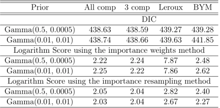
The DIC values are presented in the first row of Table 1.1. The model proposed by Leroux has the poorest fit followed by the model with all neighborhood components and the BYM model. Although they have similar values, it is clear that the model with three components is the best one for these data. In order to check the model sensitivity with respect to the choice of the prior distribution for the variance parameters, we fit the model considering a Gamma distribution with parameters 0.01 and 0.01 for these precision parameters. The values of the DIC criterion are shown in the second row of Table 1.1. The results are almost the same as before. Again, the best model is that with three components, while the BYM and Leroux models had the worst fit.
The DIC has been criticized as an inadequate measure to evaluate models and it should be considered cautiously [62]. Therefore, in addition to this global measure, we also calculated a cross-validation posterior predictive distribution check proposed by [69]. We computed the approximated conditional probability ordinate using their importance weights and the importance resampling methods. The basic idea of posterior predictive checking is to assess the fitness of the model in a given area in a two step procedure. In the first one, we obtain a predictive distribution for the i-th area without using the observed count in the area in question. In the second one, we compare the truly observed disease count in that area with the predictive distribution evaluating how extreme it is.
More specifically, let θ be the vector of all parameters in a given Bayesian model and
Y−i denote the data vector without the i-th area count. Let p(θ|Y−i) denote the posterior
cross-Prior All comp 3 comp Leroux BYM DIC
Gamma(0.5, 0.0005) 438.63 438.59 439.27 439.28 Gamma(0.01, 0.01) 438.74 438.66 439.63 441.85
Logarithm Score using the importance weights method
Gamma(0.5, 0.0005) 2.22 2.24 7.87 2.48
Gamma(0.01, 0.01) 2.25 2.22 7.86 2.62
Logarithm Score using the importance resampling method
Gamma(0.5, 0.0005) 2.05 2.04 2.82 2.40
Gamma(0.01, 0.01) 2.03 2.04 2.67 2.27
Table 1.1: DIC and Logarithm Score criteria for North Carolina data base using Gamma(0.5,0.0005) (first row) and Gamma(0.01,0.01)(second row). The models compared are BYM, Leroux and our model with all and with three components. The logarithm score criterium is evaluated with the importance weights and the importance resampling methods.
validation posterior predictive distribution of Yrep
i,−i as
CP Oi=p (
Yrep
i,−i|Y−i
) =
∫
p(Yrep
i,−i|θ)p(θ|Y−i)dθ
where Yrep
i,−i is a predicted value for the count in region ibased on the given model and data
Y−i. This measure is also called conditional predictive ordinate (CPO). A small value of the
CP Oi indicates that thei-th observation is very unlikely under the model and the remaining
observations.
As it is very costly to refit the model without each observation in turn, [69] avoid the refitting of the model using two different methods. They propose the use of importance weighting and importance resampling to approximate the posterior distribution that would be obtained if the analysis were repeated without a small area. In order to compare the observed CPO’s, we used a summary measure known as Logarithmic Score [32]. This is a scoring rule providing an evaluation of a model forecasting performance based on the posterior predictive distribution. This measure is calculated as
LS=− ∑N
i=1log(CP Oi)
N . (1.9)
The lower this value, the better the model. According to [70], this logarithm score is asymp-totically equivalent to the Akaike Information Criterion if the observations are independent.
three components, were better than the others. It is also noticeable that Leroux model had a poor performance in all the cases.
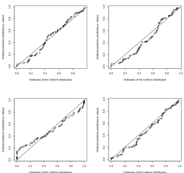
One additional cross-validation measure, proposed by [57], can be used to evaluate the goodness of fit of the models. This method is based on the simulation of both, replicate random effects and data, and it is simpler to apply than the methods from Stern and Cressie. The simplicity comes from the embedding of the leave-one-out predictive distributions replications within the MCMC simulations. The Bayesian p-value is defined as the minimum between
P(Yrep
i,−i < yi|y−i) + 12P(Yi,−irep =yi|y−i) and P(Yi,−irep > yi|y−i) +12P(Yi,−irep =yi|y−i). These
p-values should be approximately uniformly distributed if the model is correct and [57] suggested that a QQ-plot as a diagnostic tool for model checking. Figure 1.1 shows the QQ-plot for each of the models using a Gamma(0.5,0.0005) as a hyperprior while Figure 1.2 shows the same QQ-plot using a Gamma(0.01,0.01)as a hyperprior. The model proposed by Leroux is not adequate as the points clearly depart from the straight line, while the other three models have their p-values equally well fitted by the uniform distribution.
1.6.1 Including covariates
Most epidemiologic studies involve risk factors. The spatial analysis of disease rates should always take into account known or suspected risk factors. The random effects modeled with Bayesian spatial models stands for unknown risk factors and their estimation through the posterior distribution could help on spotting underlying causes for these as yet un-known risks. There is not much knowledge of the syndrome’s biological cause or poten-tial causes but some epidemiological studies have found an ecological correlation between SIDS rates and social-economic conditions (see [36]). Black, American Indian or Eskimo infants have a larger incidence of SIDS, as well as those under maternal risks such as be-ing a teenage mother, bebe-ing a smoker, drug or alcohol user, and havbe-ing inadequate prena-tal care. Therefore, we included the following covariates in our model: the average pro-portion of Black and American Indians in the county population from 2001 to 2009 (see
http://www.census.gov/popest/counties/asrh/CC-EST2009-RACE5.html), the proportion
of mothers who had prenatal care and the proportion of mothers who were smokers from 2005 to 2009 (see http://www.epi.state.nc.us/SCHS/data/databook/).
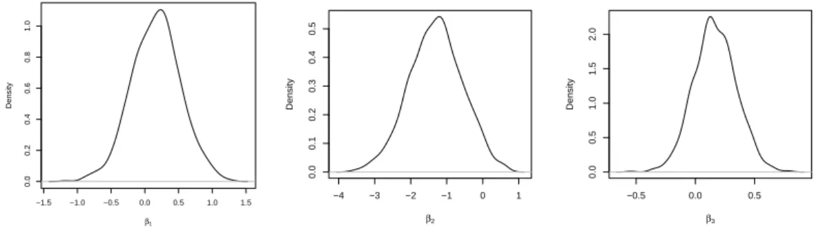
We centered all three covariates and fitted the all components model with the three covari-ates simultaneously present in the model. We obtained the posterior densities in Figure 1.3. Fitting our model with three components gave virtually the same result. We find evidence of covariate effects only for the proportion of mothers who had prenatal care (second plot), since zero is on the border of the 95% highest density interval (given by (−2.719,0.139)) and the posterior probability that the covariate coefficient is less than zero is given by 0.963. We refit-ted the model three times, each time with a single covariate and the only significant covariate was again the proportion of mothers who had prenatal care. Focusing on the model with this single covariate, we obtain a posterior mean equal to −1.419. This means that a 1% increase in prenatal care leads to an average reduction in the SIDS risk of exp(−1.419∗0.01) = 0.987
0.0 0.2 0.4 0.6 0.8
0.0
0.2
0.4
0.6
0.8
1.0
Ordinates of the Uniform distribution
Ordered poster
ior predictiv
e p−v
alues
0.0 0.2 0.4 0.6 0.8 1.0
0.0
0.2
0.4
0.6
0.8
1.0
Ordinates of the Uniform distribution
Ordered poster
ior predictiv
e p−v
alues
0.0 0.2 0.4 0.6 0.8 1.0
0.0
0.2
0.4
0.6
0.8
1.0
Ordinates of the Uniform distribution
Ordered poster
ior predictiv
e p−v
alues
0.0 0.2 0.4 0.6 0.8 1.0
0.0
0.2
0.4
0.6
0.8
1.0
Ordinates of the Uniform distribution
Ordered poster
ior predictiv
e p−v
alues
Figure 1.1: QQ-plot of p-values using Gamma(0.5, 0.0005) for all components, three com-ponents, Leroux and Bym models. The p-values were calculated using the cross-validation proposal of [57].
1.7 Simulation study
In this section, we present a simulation study that helps to understand our formulation bet-ter and that shows clearly its advantages and benefits with respect to the other two main approaches available to spatial statisticians, the Leroux and the BYM models. We used the North Carolina counties with the observed live births in the period 1999-2006. The precision coefficient σ2 is fixed and equal to 5 in all simulations. The simulated SIDS counts were generated according to six different scenarios, as we explain next.
The first model for the SIDS counts assumed an extreme situation, in which we have a constant underlying rate equal to the observed NC SIDS rate (0.73 per thousand live births). That is, each yi is generated independently from a Poisson distribution with mean Ei = 0.73mi/1000, where mi is the observed number of live births in the i-th county. This implies
0.0 0.2 0.4 0.6 0.8 1.0
0.0
0.2
0.4
0.6
0.8
1.0
Ordinates of the Uniform distribution
Ordered poster
ior predictiv
e p−v
alues
0.0 0.2 0.4 0.6 0.8 1.0
0.0
0.2
0.4
0.6
0.8
1.0
Ordinates of the Uniform distribution
Ordered poster
ior predictiv
e p−v
alues
0.0 0.2 0.4 0.6 0.8 1.0
0.0
0.2
0.4
0.6
0.8
1.0
Ordinates of the Uniform distribution
Ordered poster
ior predictiv
e p−v
alues
0.0 0.2 0.4 0.6 0.8 1.0
0.0
0.2
0.4
0.6
0.8
1.0
Ordinates of the Uniform distribution
Ordered poster
ior predictiv
e p−v
alues
Figure 1.2: QQ-plot of p-values using Gamma(0.01, 0.01) for all components, three com-ponents, Leroux and Bym models. The p-values were calculated using the cross-validation proposal of [57].
and had spatially varying relative risks. In these other cases, yi was simulated independently
from a Poisson with mean Eiψi where ψi = exp(bi). In the second scenario, ψi ≈ 1 for
all i, implying that the precision matrix is composed basically by the neighborhood matrix full of 1’s. More specifically, bi follows our model with λ20 = 0.979 and λ1 = . . . = λ19 =
(1−λ20)/19 = 0.001.
In the third scenario, we used our component model with four heavily weighted neighbor-hood matrices in the precision matrix: the identity matrix, the first and the second neigh-borhood order matrices, and the matrix full of 1’s, with λ1 = 0.007,λ2 = 0.421,λ3 = 0.351,
and λ20 = 0.210. All the other λ’s are small and equal to 0.001. The fourth scenario had
a high weight associated with the second neighborhood order matrix, and moderate weights associated with the identity and the matrix full of 1’s. That is, λ1 = 0.108, λ2 = 0.011,
−1.5 −1.0 −0.5 0.0 0.5 1.0 1.5
0.0
0.2
0.4
0.6
0.8
1.0
β1
Density
−4 −3 −2 −1 0 1
0.0
0.1
0.2
0.3
0.4
0.5
β2
Density
−0.5 0.0 0.5
0.0
0.5
1.0
1.5
2.0
β3
Density
Figure 1.3: Posterior density of the β coefficients for three covariates using our model with all components for the spatial random effect. The first plot refers to the proportion of Black and American Indians in the population, the second plot refers to proportion of mothers who had prenatal care and the third plot refers to the proportion of mothers who were smokers.
Leroux model with λ1 = λ2 = 0.5 and all the other λ’s equal to zero. The sixth scenario
follows a CAR model with ρ= 0.99 to mimic the behavior of the improper ICAR prior. We fitted four different models to each simulated dataset: our model with 20 increasing neighborhood orders, our model with three components (described in Section 1.5.1), and the BYM and Leroux models. The prior distribution for the precision parameter was taken as a Gamma(0.5,0.0005) in all models. In all cases, we ran the MCMC for 3000 iterations with 1500 as a burn-in period.
Let
M SEi = 1
B
B ∑
j=1
(ψ(ij)−exp(bi))2.
whereψi(j)is thej-th simulated value of the relative riskψi,exp(bi)is the realized relative risk
under each one of the scenarios, and B is the number of simulations retained after burn-in. Note that bi = 0 in the first scenario. Denote by M SE the average of the M SEi values,
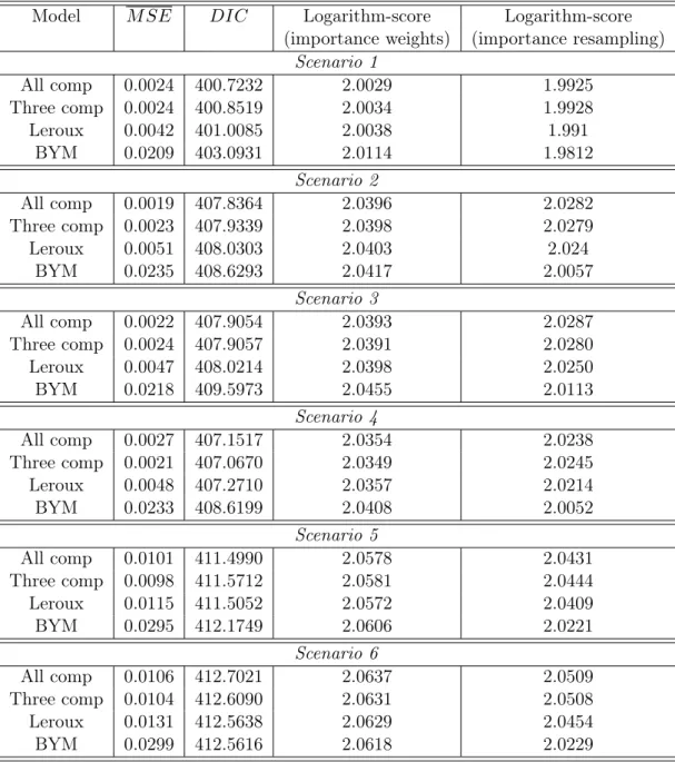
i = 1, . . . ,100. We considered four summary statistics to evaluate the fitted models: the average M SE, the DIC, and the two logarithm scores, based on importance weights and on importance resampling. The measure M SE is our preferred criterium to select the best model since we compare the estimated with the true relative risks in each model. Of course, this is only possible in simulations, not in real data analysis. We simulated 10 independent copies of each scenario. The results shown below are the averages of the summary statistics in these 10 independent replications.
Table 1.2 shows the values of these evaluation measures for each one of the four possible models in each scenario. Considering theM SEcriterium, our models are always the best one, either the three components model or the 20 components model. This is rather surprising considering that at least in one case (Scenario 5), we are fitting a model (Leroux) to data generated according to this same model. It is also clear that the BYM model is the worst model in all scenarios. In all of them the three component model had almost the same M SE