Maria da Conceição Figueiredo, Elsa Fontainha
Male and Female Wage Functions:
A Quantile Regression Analysis using LEED and LFS Portuguese Databases
WP01/2015/DE
_________________________________________________________
De pa rtme nt o f Ec o no mic s
W
ORKINGP
APERS1 Male and Female Wage Functions:
A Quantile Regression Analysis using LEED and LFS Portuguese Databases
Maria da Conceição Figueiredo1
Elsa Fontainha2
Abstract§
The research aims to study the distribution of hourly wages for men and women in Portugal, adopting a quantile regression (QR) approach. Two databases are used for the estimation of the wage functions: the Quadros de Pessoal, Linked Employer-Employee Data (QP-LEED) and the Inquérito ao
Emprego, Portuguese Labour Force Survey (IE-LFS).
Three basic models are considered to explain the hourly wages for men and women: the first model, using each database separately, is estimated adopting education, tenure, potential experience, activity sector, and job as independent variables; the second, using data from QP-LEED, includes additional determinants related to firm (firm size and foreign social capital); and the third, using data from the IE-LFS, includes additional independent variables related to the worker's family (marital status and children).
The results indicate that: (i) Regardless of the database used, the quantile regression (QR) shows superiority over OLS approach; (ii) In general, the same model specification estimated using each database - one administrative (QP-LEED), and the other based on a survey (IE-LFS) - present convergent results; (iii) Independently of the database used, the equations for men and for women reveal that the levels of education have a higher impact on wage determination; (iv) In general, the variables related to the firm contribute to the explanation of wages of men and women while those related to family only contribute to the explanation of men's wages; and (v) the clear different returns for the same characteristics found between men and women, and the pattern of differences which increase across quantiles strongly indicates that the present study should continue in the future, with the analysis of the explanation of the gender wage gap.
JEL code: J31, C21
Keywords: wage function; quantile regression; Linked Employer-Employee Data; Labour Force Survey; male-female wage differences
1 BRU-ISCTE-IUL ISCTE – IUL Lisbon University Institute; [email protected]
2
1. Introduction
This research intends to attain two goals: to explain and compare wages of men and women in Portugal and to contrast the results obtained from two separate databases. To achieve the first goal, a quantile regression approach is adopted. About the second goal, as far as the authors know, this is the first attempt to compare results obtained from two distinct databases, both of which provide useful information to explain wage levels and wage differences.
The Mincerian wage equation (Mincer, 1974) included as dependent variable the logarithm of the hourly wage and as explanatory variables factors associated with the human capital characteristics (e.g. years of schooling, potential experience, tenure). Since that seminal work, the list of explanatory variables has been extended with variables associated with supply like gender, marital status, number of children and children age, cognitive skills, social capital and networks, race and ethnicity, specialization between market and non-market work, beauty, psychological capital (Balcar, 2012). Variables associated with demand and institutional framework like sector of activity, firm characteristics (e.g. size, location), occupation, unionization, minimum wage, family policies, have been also added.
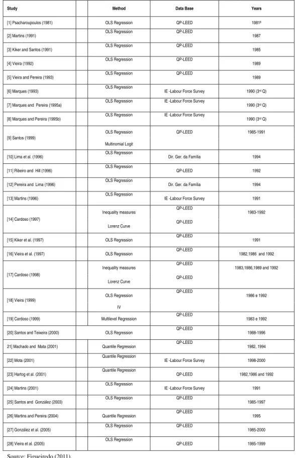
Most of the research on Portuguese wages and wage inequality is based on the Quadros de Pessoal (QP-LEED)3. In Appendix (Table A1) 37 empirical studies are identified
that analyze the Portuguese case. Only ten of them use other than QP_LEED database and seven of these are based on the Labour Force Survey (Figueiredo, 2011). A previous literature review, (Pereira and Lima, 1999) also show the predominance of use of QP-LEED database. Figueiredo (2011) has studied the wage function and the gender wage gap decomposition based on Inquérito ao Emprego, Portuguese Labour Force Survey (IE-LFS).
The present paper is a preliminary step for the study of that wage gap based on Quadros de
Pessoal Linked Employer-Employee data (QP-LEED). Here the wage functions for men and
women are analyzed using the two databases: (IE-LFS) and (QP-LEED).
The paper is organized as follows: in Section 2 the option for quantile regression is justified, the two data sources harmonization is presented and different specifications for
3
3
wage function are introduced. Section 3 presents and discusses the results. The last section lists the main conclusions and suggests future research avenues.
2. Empirical Strategy and Databases Harmonization
2.1. Quantile Regression (QR) Analysis
Unlike the Multiple Linear Regression model, in which it is only possible to know the effects of the explanatory variables in the mean of the conditional distribution of dependent variable, the Quantile Regression (QR) allows estimation of the effects of covariates on different points of the dependent variable distribution. Buchinsky (1998a, p.89) referred as an useful feature of QR that “... potentially different solutions at distinct quantiles may be interpreted as differences in the response of the dependent variable to changes in the regressors at various points in the conditional distribution of the dependent variable”. Thus, QR permits a full characterization of the conditional distribution of wages, controlling for individual heterogeneity associated with this type of data.
The linear model of Quantile Regression is presented as:
1, … , e (1)
where N is the sample size, is the dependent variable, is a vector of 1 size of the
explanatory variables, is the vector of 1 size of the regression parameters associated with the θ-th percentile, and corresponds to the error term.
This model assumes the following for the random residual variable ( ) :
Consequently the quantile of order of conditional in is given by
This means that it is linear in . Therefore, it should be noted that the marginal effects of covariates, given by , in principle, differ across quantiles. From the last expression it follows that is the partial derivative of the conditional quantile function in relation to the explanatory variables. As a result it is possible to obtain the marginal effects at different points of the conditional distribution.
,
´i i
i
x
u
y
0,1, 0 ) | (u i xi
Q
|
´
0,1 yi xi xi
Q
i
4
Quantile regression does not impose assumptions about the parametric distribution errors. Consequently, the quantile regression model overcomes the restrictive assumption present in the linear regression model, where the error terms are independent and identically distributed in the conditional distribution.
The vector of estimated parameters for a given θ, , is obtained as a solution of a minimization problem (Buchinsky, 1998b) of the weighted sum of the absolute value of the errors.
2.2. Databases Harmonization and Sample Characteristics
2.2.1. Linked Employee Employer Data and Portuguese Labor Force Survey
Quadros de Pessoal, LEED data is an administrative annual database collected by the
Ministry of Labour/Employment. It assembles information from all workers and firms (including micro firms) and excludes the civil servants. The data presented in this paper refer to October 2007.
Portuguese Labour Force Survey-LFS (Inquérito ao Emprego) is a statistical database
collected by Statistics Portugal and is part of the European Labour Force Survey- Eurostat4.
Is a household sample quarterly survey collecting information on persons in the labour force and outside the labour force. The unemployment rate in EU countries is computed based on LFS data.
2.2.2. Sample and Sample Characteristics
The two samples selected for the present research include wage earners, between 15 and 64 years old, working between 30 and 50 hours per week, employed in private sector. Several sectors were excluded from the analysis: Agriculture, Forestry, Fishing, Public Administration Security and Social Security, Education, Health and Social Work, Construction and Domestic Services.
Table A2 presents the descriptions of the variables. Table 1 presents descriptive statistics from the two samples, obtained each from the two data sources. The main difference
4 http://ec.europa.eu/eurostat/web/microdata/european-union-labour-force-survey
argmin1
1
ˆ '
: :
'
'
'
i i
x y i x
y i
i
i x y x
y
5
between the data sources results is the mean of the hourly wage (wagehr): the mean obtained
with the QP-LEED data is higher. This result was expectable because the wage in QP-LEED is the wage before taxes and in IE-LFS is the wage net from taxes. Potential experience
(experience_pot) is slightly higher in the case of IE-LFS. Note that the IE-LFS has also
information about the effective experience5 (experience_eff ). The values for tenure (tenure)
are higher in IE-LFS.
Table 1 – Summary Statistics (All; Male; Female; IE-LFS and QP-LEED)
Source : IE-LFS Source : QP-LEED Source:
IE-LFS Source: QP-LEED
All (N=4367) (N=2299) Male (N=2068) Female All (N=5073) (N=2881) Male (N=2192) Female Female Male/ Female Male/
Mean SD Mean SD Mean SD Mean SD Mean SD Mean SD (mean) (mean)
wagehr6 4.2425 2.5306 4.7546 2.84675 3.6733 1.97514 6.74 6.4351 7.65 7.5185 5.5392 4.36244 1.29 1.38
male 0.53 0.4990 1.00 0.0000 0.00 0.0000 0.57 0.4950 1.00 0.0000 0.00 0.0000 1 1
edu1 0.02 0.1280 0.01 0.1080 0.02 0.1480 0.01 0.1090 0.01 0.1110 0.01 0.1060 0.50 1.00
edu2 0.24 0.4270 0.25 0.4310 0.23 0.4210 0.19 0.3900 0.18 0.3820 0.20 0.4000 1.09 0.90
edu3 0.24 0.4260 0.24 0.4290 0.23 0.4240 0.20 0.4010 0.21 0.4110 0.18 0.3870 1.04 1.17
edu4 0.24 0.4270 0.26 0.4410 0.21 0.4100 0.22 0.4160 0.24 0.4280 0.20 0.3990 1.24 1.20
edu5 0.17 0.3800 0.15 0.3580 0.20 0.4010 0.24 0.4280 0.22 0.4170 0.26 0.4400 0.75 0.85
edu6 0.02 0.1460 0.02 0.1370 0.02 0.1550 0.02 0.1500 0.02 0.1460 0.02 0.1550 1.00 1.00
edu7 0.07 0.2520 0.06 0.2430 0.07 0.2620 0.11 0.3166 0.11 0.3104 0.12 0.3245 0.86 0.90
experience_pot 22.35 11.9670 23.17 12.2080 21.44 11.6290 20.97 11.4200 21.75 11.6530 19.95 11.0260 1.08 1.09
experience_sq 642.75 573.3080 685.69 591.2370 595.02 548.9060 570.28 538.1340 608.89 561.0520 519.54 502.0660 1.15 1.17
tenure 10.76 10.0211 11.51 10.4964 9.93 9.3972 8.28 9.0120 8.82 9.4650 7.56 8.3280 1.16 1.17
tenure_sq 216.28 344.5091 242.72 366.3914 186.89 315.9236 149.70 277.9470 167.35 300.3160 126.50 243.5950 1.30 1.32
married 0.68 0.4660 0.69 0.4620 0.67 0.4710 n.a. n.a. n.a. n.a. n.a. n.a. 1.03 n.a.
Child <6 0.03 0.1750 0.03 0.1730 0.03 0.1770 n.a. n.a. n.a. n.a. n.a. n.a. 1.00 n.a.
Child 6_17 0.43 0.6650 0.41 0.6570 0.44 0.6730 n.a. n.a. n.a. n.a. n.a. n.a. 0.93 n.a.
Child >17 0.28 0.5760 0.29 0.5790 0.28 0.5730 n.a. n.a. n.a. n.a. n.a. n.a. 1.04 n.a.
experience_eff 21.85 13.0444 23.07 13.4587 20.51 12.4330 n.a. n.a. n.a. n.a. n.a. n.a. 1.12 n.a.
age 38.56 11.3930 39.25 11.7640 37.79 10.9180 37.75 10.6160 38.43 10.9620 36.86 10.075 1.04 1.04
size_med n.a. n.a. n.a. n.a. n.a. n.a. 0.30 0.4600 0.30 0.4580 0.31 0.4620 n.a. 0.97
size_lar n.a. n.a. n.a. n.a. n.a. n.a. 0.36 0.4810 0.36 0.4810 0.37 0.4820 n.a. 0.97
capext_5 n.a. n.a. n.a. n.a. n.a. n.a. 0.04 0.1900 0.04 0.1970 0.03 0.1790 n.a. 1.33
capext_1 n.a. n.a. n.a. n.a. n.a. n.a. 0.16 0.3700 0.16 0.3620 0.18 0.3800 n.a. 0.89
Source: Authors computations based on LEED-QP 2007 and LFS-IE 2007.
5 The 2007 Portuguese Labour Force Survey (IE-LFS) includes the question: “On what date you began working for the first time?”. In fact, this is not a perfect measure of effective experience because is not possible to identify if there were breaks after the first job and the duration of those breaks. This is a better measure of experience but is still a proxy. The models were estimated (not shown here) using the effective experience instead of potential experience without relevant differences of results.
6
The comparison of the means for male and female (the last two columns of Table 1 present the ratio of means male/female) shown that the main differences are related with hourly wages (wagehr). On average, men have a higher salary compared with women: 38% higher using the QP-LEED data, and 29% higher using the IE-LFS data. This difference could possibly be explained partially by non-proportional taxes on wages. It is likely that highest values of the standard deviations of the hourly wages (Table 2) result from the progressiveness of taxes.
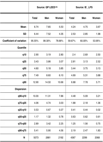
Regardless of the database used, the distribution of hourly wages over the five quantiles (Table 2) is different. This different structure across quantiles can justify the need to perform the analysis not only on the average (for which the OLS regression would be suitable) but rather along the distribution. Consequently, the Quantile Regression (QR) approach is more appropriate and is adopted.
Table 2 – Hourly Wage Distribution
Source: QP LEED (b) Source: IE _LFS
Total Men Women Total Men Women
Mean 6.74 7.65 5.53 4.24 4.75 3.67
SD 6.44 7.52 4.35 2.53 2.85 1.98
Coefficient of variation 95.55% 98.30% 78.66% 59.67% 60.00% 53.95%
Quantile
q10 2.90 3.19 2.80 2.4 2.69 2.50
q25 3.43 3.86 3.07 2.81 3.13 2.52
q50 4.60 5.18 3.85 3.44 3.75 3.13
q75 7.49 8.60 6.10 4.69 5.31 3.88
q90 12.90 14.50 10.66 6.88 7.78 5.71
Dispersion
q90-q10 10.00 11.31 7.86 4.48 5.09 3.21
q75-q25 4.06 4.74 3.03 1.88 2.18 1.36
q25-q10 0.53 0.67 0.27 0.41 0.44 0.02
q50-q25 1.17 1.32 0.78 0.63 0.62 0.61
q75-q50 2.89 3.42 2.25 1.25 1.56 0.75
q90-q75 5.41 5.90 4.56 2.19 2.47 1.83
N 5073 2881 2192 4367 2299 2068
7
2. 3. QR Model Specification
The empirical strategy followed several steps. Firstly, a linear model is estimated using the OLS and the full samples (males and females) for each of the two databases (QP-LEED and IE-LFS) and using the same specification. Secondly, the wage function is estimated separately for males and females using each database, the same specification and OLS. Thirdly, the same wage function specification is estimated separately for males and females using quantile regression (QR). Fourthly, firm variables are added to both equations, based on QP-LEED data and using QR methodology. Finally family variables are added to both regressions (males and females), based on IE-LFS data and adopting QR analysis.
Initially, we used the specification of the linear model introduced by Mincer (1974). The specification of the wage functions includes experience (actual or potential) and tenure. Both, experience and tenure are specified in linear and quadratic terms to capture the nonlinear effects. For each of the two databases (QP and LFS), the traditional Mincerian wage functions were estimated first considering the pooled sample (including as explanatory the binary male), and then separately by gender. Table A2 presents the definitions of the
variables. Considering the male and female pooled sample, it is assumed that the effect of
male variable is independent from other individual characteristics (e.g. experience and
education). However, it is likely that men are paid for their characteristics differently from women. Consequently, it is too restrictive to assume that the estimated coefficients associated with the regressors are held constant by gender. Therefore, we proceeded to estimate the wage equations separately for men and for women7.
Because the heteroscedasticity tests performed to regressions in the mean showed that the errors are heteroscedastic, the OLS estimation was carried out with the option standard errors robust to heteroscedasticity, and the estimates for the standard errors of quantile regressions were obtained using the bootstrap technique. The calculations were carried out with 1,000 replicates, this being the usual number of replicas suggested by Davidson and Hinkley (1997). This value is acceptable taking into account that, according to the three step method presented by Andrews and Buchinsky (2000), the optimal number
7 As reported by Verbeek (2004), another solution - that would lead to similar results – would be to consider the interaction of the variable
gender, multiplying the covariates by the gender variable. Although, the standard errors are homoscedastic in the pooled sample. In the case of estimating the model separately for the two subsamples of men and women, we assume that the error terms are homoscedastic within each sub-sample.
8
of replicas obtained varied between 800 and 1,000, depending on the regression quantile estimate. Computations use Stata 12.0 software.
The group of models labeled as Model 1 includes as explanatory variables: the
gender (only when all the sample is used), education (taking the zero years of schooling –
edu1- as reference category), experience, tenure, sector of activity (financial activities is the
reference category), and occupation (clerk, admistritative workers is the reference category). Model 2 additionally includes the size of the firm ( the reference category is
small firms)and the percentage of foreign capital in social capital (the reference category is without foreign social capital). Model 3 additionally includes civil status and the existence of children by age group.
The models studied are the following:
Models 1
OLS regression (All)
OLS regression by gender
Quantile Regression (All)
Quantile Regression by gender
Model 2
Quantile Regression with additional firm variables (source: QP-LEED)
sec
exp exp | 40 33 32 32 12 11 2 11 10 2 9 8 7 2 1 1 0 u job tor tenure tenure educ male x Q
j j j
j j j
j j j
sec
exp exp | 39 32 31 31 11 10 2 10 9 2 8 7 6 1 0 g j j g j j j g j g g g g j j g j g g g u job tor tenure tenure educ x Q
sec exp exp 40 33 32 32 12 11 2 11 10 2 9 8 7 2 1 10 male educ tenure tenure tor job u
j j j j j j j j
j
sec exp exp 39 32 31 31 11 10 2 10 9 2 8 7 6 1 0 g j j g j j j g j g g g g j j g j g g u job otr tenure tenure
educ
sec
exp exp | 43 42 41 41
40 ~39 31
9
Model 3
Quantile Regression with family variables (source: IE-LFS)
3. Results and Discussion
Model 1
The OLS regression and the QR applied to the total samples impose the condition that the returns from the individual characteristics are assumed to be the same either for men or for women. In these regressions, the estimated coefficient associated to the dummy variable
male, indicates the magnitude of discrimination, it means, the extent to which the wage gap
between men and women remains unjustified in the average and in the different quantiles,
after controlling for individual differences in the various combinations of characteristics.
Cardoso (2007) draws attention to the fact that because the regression controls for a broad set of factors, it is possible that some determinants of differentiation are not being raised and the value cannot be considered an exact measure of discrimination in the labor market. Consequently, in results analysis it is important to note the set of variables included in the regression, because uncontrolled variables may exist. The first line in Table 3 shows that men earn on average wages which are 18.11% higher than women wages who own comparable individual characteristics. The results obtained using IE-LFS data are very similar (17.78%) to those obtained with QP-LEED. The estimated coefficients (0.1811 and 0.1778, respectively using QP-LEED and IE-LFS databases) do not show a real picture of the differences between men and women wages, on the contrary, they provide a biased image, because they present a central value in relation to the entire distribution.
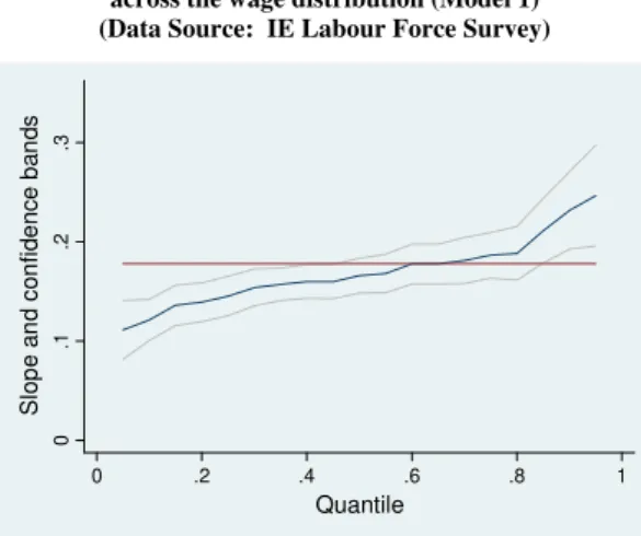
Figures 1 and 2, representing the effect of gender on hourly wages across the wage distribution, allow a better understanding of that bias. The Figure 1 (based on QP-LEED) shows that in quantile 10 men's wages are just 10.02% higher than those of women, but in
sec 5 17 18
exp exp
|
42 41
40 39
32 31
31
11 10
2 10
9 2 8 7
6
1 0
g g
g g
j
j g j j
j g
j
g g
g g
j
j g j g
g g
u child child
child job
tor
tenure tenure
educ x
Q
10
quantile 50 the difference is 17.8% and in quantile 90 reaches the value of 27.5 %. Figure 2 (based on IE-LFS) also presents the impact of gender on the distribution of wages, and reveals a similar behavior across quantiles (12.1%, 16.6% and 23.2% respectively in q10, q50 and q90). The figures above illustrate the limits of the wage approach on the mean. In fact, as argued by Buchinsky (1994, p. 453) “’on the average’ has never been a satisfactory statement with which to conclude a study on heterogeneous populations. Characterization of the conditional mean constitutes only a limited aspect of possibly more extensive changes involving the entire distribution”
Figure 1 - The effect of gender on hourly wages across the wage distribution (Model 1)
(Data source: QP LEED)
Source: Authors computations based on QP-LEED 2007.
Figure 2 – The effect of gender on hourly wages across the wage distribution (Model 1) (Data Source: IE Labour Force Survey)
Source: Authors computations based on IE-LFS 2007.
The potential experience (linear and squared terms reveals a differential effect between men and women through the quantiles (Tables 3 to 5; Model 1). Once again, the
return obtained by men is higher than the return obtained by women. Analyzing the tenure
(tenure and tenuresq variables), it is found that the coefficients have the expected effect and
are statistically significant, although low, revealing very low effect on wages for both men and women, and in both databases used. Furthermore, contrary to other variables, the tenure behavior remains in general uniform through the distribution for men and for women. The results obtained for experience and tenure converge with those obtained by Machado and Mata (2001, p. 124-125) for 1982 and 1994: the linear and the squared term of experience are significant at all quantiles and, for the tenure the squared term is non-significant at top quantiles. That is precisely what happens in IE-LFS, both for men and for women. However, using the QP-LEED that behavior does not occur.
0
.1
.2
.3
S
lo
p
e
a
n
d
co
nf
id
en
ce
ba
nd
s
0 .2 .4 .6 .8 1
Quantile
0
.1
.2
.3
S
lop
e an
d c
o
n
fi
d
e
n
c
e
b
a
n
d
s
0 .2 .4 .6 .8 1
11
The lower significance of squared term of tenure (tenure_sq) was also found by
Fitzenberger and Kurtz (2003, p.494) for Germany, using the German Socioeconomic Panel (GSOEP) data. They conclude that experience shows the usual concave profiles at all quantiles, whereas the tenure effect is almost linear at all quantiles and insignificant at q90.
Making a comparison by gender, in the mean or in each quantile, the marginal effects of experience and tenure are higher for men than for women regardless the database used (Tables 3 to 5). However, the coefficients associated with tenure are different depending on the database used (Tables 3 to 5). It is likely that this result reflects the different age means within the samples (by gender) and between the samples: in QP-LEED the average age for men is 38.43 years and for women 36.86; in IE-LFS, the values are respectively 39.25 and 37.79 (Table 1).
Table 3 - Quantile Regression Estimations Model 1 (All; Sources: QP-LEED and IE-LFS)
QP-LEED_All IE-LFS_All
OLS q10 q50 q90 OLS q10 q50 q90
Coef SD Coef SD Coef SD Coef SD Coef SD Coef SD Coef SD Coef SD
male 0,1811* 0.0105 0,1002* 0.0124 0,1779* 0.0119 0,2748* 0.0213 0,1778* 0.0091 0,1213* 0.0108 0,1658* 0.0100 0,2317* 0.0207
edu2 0.0570 0.0354 0.0289 0.0501 0.0779 0.0549 0.0476 0.0997 0,0721* 0.0246 0,0494*** 0.0285 0,0636** 0.0307 0,0961*** 0.0513
edu3 0,1247* 0.0359 0.0778 0.0511 0,1548* 0.0555 0.1388 0.0997 0,1696* 0.0257 0,0868** 0.0281 0,1606* 0.0317 0,1935* 0.0524
edu4 0,2571* 0.0367 0,1932* 0.0527 0,2707* 0.0567 0,2397** 0.0989 0,2574* 0.0266 0,1515* 0.0305 0,2337* 0.0327 0,2932* 0.0555
edu5 0,4033* 0.0388 0,2637* 0.0534 0,3833* 0.0594 0,4818* 0.1030 0,3776* 0.0289 0,2391* 0.0335 0,3554* 0.0340 0,4105* 0.0589
edu6 0,6241* 0.0566 0,4422* 0.0799 0,5827* 0.0840 0,7835* 0.1193 0,5101* 0.0444 0,2946* 0.0484 0,4752* 0.0503 0,5623* 0.1006
edu7 0,7896* 0.0470 0,5726* 0.0661 0,7577* 0.0700 0,9136* 0.1098 0,7003* 0.0405 0,442* 0.0454 0,6404* 0.0464 0,8513* 0.0873
experience_pot 0,0241* 0.0020 0,0136* 0.0027 0,0209* 0.0022 0,0295* 0.0037 0,0239* 0.0016 0,017* 0.0018 0,0207* 0.0016 0,0279* 0.0031
experience_sq -0,0004* 0.0000 -0,0002* 0.0001 -0,0003* 0.0000 -0,0003* 0.0001 -0,0003* 0.0000 -0,0003* 0.0000 -0,0003* 0.0000 -0,0004* 0.0001
tenure 0,022* 0.0017 0,0217* 0.0022 0,0196* 0.0019 0,0176* 0.0040 0,0108* 0.0014 0,0071* 0.0014 0,0100* 0.0014 0,0110* 0.0030
tenure_sq -0,0004* 0.0001 -0,0004* 0.0001 -0,0003* 0.0001 -0,0003** 0.0001 -0,0001* 0.0000 -0,0001** 0.0000 -0,0001* 0.0000 -0,0001*** 0.0001
R^2/PseudoR^2 0.6717 0.2705 0.445 0.5029 0.6078 0.1905 0.3735 0.4689
N 5073 4367
Source: Authors computations based on QP-LEED 2007 and IE-LFS 2007. Note: (*) p<0.01; (**) p<0.05; (***) p<0.10
Occupations and sectors were also studied. In general, the results obtained from each data base converge (Figures A1 and A2). We plan to deepen our understanding of the reasons for the differences found among occupation and industries in future research.
12
Table 4 - Quantile Regression Estimations Model 1 (Men and Women; Source: QP-LEED)
QP_male QP_female
OLS q10 q50 q90 OLS q10 q50 q90
Coef SD Coef SD Coef SD Coef SD Coef SD Coef SD Coef SD Coef SD
edu2 0,108** 0.0499 0.0579 0.0903 0,1095*** 0.0576 0,2329*** 0.122 -0.0035 0.0485 0.0137 0.0513 -0.0148 0.0544 -0.0638 0.0906
edu3 0,1559* 0.0499 0.089 0.0896 0,1807* 0.0591 0,2625** 0.1229 0,084*** 0.0499 0.0586 0.0534 0.052 0.0558 0.0488 0.0959
edu4 0,3094* 0.0506 0,2298** 0.0921 0,2946* 0.0595 0,4021* 0.1202 0,1811* 0.0514 0,1279** 0.0563 0,1258** 0.0565 0.1517 0.0973
edu5 0,4326* 0.0533 0,3* 0.0919 0,4005* 0.0629 0,575* 0.1275 0,3451* 0.055 0,2154* 0.0605 0,2484* 0.061 0,3543* 0.1076
edu6 0,7343* 0.0863 0,5695* 0.1292 0,6815* 0.133 0,9858* 0.1672 0,4885* 0.0707 0,3491* 0.1 0,3942* 0.0866 0,5398* 0.1405
edu7 0,8618* 0.0664 0,64* 0.1055 0,8095* 0.0849 1,0764* 0.1451 0,6826* 0.0652 0,5179* 0.0832 0,5396* 0.0797 0,7193* 0.1205
experience_pot 0,0283* 0.0029 0,0176* 0.0035 0,0243* 0.0029 0,037* 0.006 0,0204* 0.0026 0,0099* 0.0031 0,0144P 0.0029 0,0208* 0.0044
experience_sq -0,0004* 0.0001 -0,0003* 0.0001 -0,0003* 0.0001 -0,0004* 0.0001 -0,0003* 0.0001 -0,0001** 0.0001 -0,0002* 0.0001 -0,0002** 0.0001
tenure 0,0223* 0.0024 0,0249* 0.0032 0,0194* 0.0027 0,0179* 0.0054 0,0212* 0.0023 0,0189* 0.0027 0,0174* 0.0022 0,0173* 0.0048
tenure_sq -0,0004* 0.0001 -0,0004* 0.0001 -0,0003* 0.0001 -0,0004** 0.0002 -0,0004* 0.0001 -0,0004* 0.0001 -0,0003* 0.0001 -0,0003*** 0.0002
R2/PseudoR2 0.6237 0.2581 0,4029* 0.4666 0.7199 0.2711 0.4768 0.5633
N 2881 2192
Source: Authors computations based on QP-LEED 2007. Note: (*) p<0.01; (**) p<0.05; (***) p<0.10
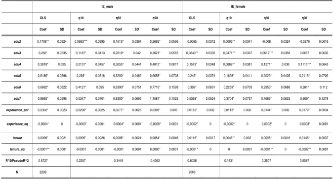
Table 5 - Quantile Regression Estimations Model 1 (Men and Women; Source: IE-LFS)
IE_male IE_female
OLS q10 q50 q90 OLS q10 q50 q90
Coef SD Coef SD Coef SD Coef SD Coef SD Coef SD Coef SD Coef SD
edu2 0,1708** 0.0324 0,0683*** 0.0395 0,1613* 0.0394 0,2662* 0.0596 0.0085 0.0312 0,0093** 0.0341 -0.008 0.0324 -0.0276 0.0616
edu3 0,282* 0.0335 0,1187* 0.0413 0,2819* 0.042 0,3621* 0.0565 0,0843** 0.0332 0,0471** 0.0337 0,0612*** 0.0358 0.0657 0.0633
edu4 0,3818* 0.035 0,2131* 0.0457 0,3655* 0.0441 0,4815* 0.0617 0,1579* 0.0348 0,0889** 0.0361 0,1271* 0.036 0,1115*** 0.0645
edu5 0,5185* 0.0396 0,293* 0.0518 0,5200* 0.0483 0,6658* 0.0708 0,245* 0.0374 0,1698* 0.0411 0,2029* 0.0405 0,2115* 0.0709
edu6 0,6662* 0.0622 0,4121* 0.095 0,6390* 0.0751 0,7716* 0.1598 0,369* 0.0601 0,2239* 0.0703 0,2953* 0.0686 0,381* 0.112
edu7 0,8665* 0.0595 0,5347* 0.0701 0,8300* 0.0693 1,1581* 0.1025 0,5368* 0.0524 0,3704* 0.0737 0,4669* 0.0633 0,609* 0.1278
experience_pot 0,0302* 0.0023 0,0208* 0.0025 0,0277* 0.0026 0,0396* 0.005 0,0163* 0.002 0,0113* 0.002 0,0144* 0.002 0,0179* 0.0034
experience_sq -0,0004* 0 -0,0003* 0.0001 -0,0004* 0.0001 -0,0006* 0.0001 -0,0002* 0 -0,0002* 0 -0,0002* 0 -0,0003* 0.0001
tenure 0,0096* 0.0021 0,0095* 0.0026 0,0088* 0.0024 0,0054* 0.0046 0,0116* 0.0017 0,0046** 0.002 0,0098* 0.0016 0,0148* 0.0037
tenure_sq -0,0001** 0.0001 -0.0001 0.0001 -0.0001 0.0001 0,0000* 0.0001 -0,0001* 0 0 0.0001 -0,0001** 0 -0,0002** 0.0001
R^2/PseudoR^2 0.5727 0.2257 0.3449 0.4362 0.6026 0.1531 0.3507 0.5087
N 2299 2068
13 Table 6 - Quantile Regression Estimations Model 2(a) (Men and Women; Source: QP-LEED)
Male (QP-LEED) Female (QP-LEED)
OLS q10 q50 q90 OLS q10 q50 q90
Coef SD Coef SD Coef SD Coef SD Coef SD Coef SD Coef SD Coef SD
edu2 0,0976** 0.0472 0.0623 0.0688 0,1095*** 0.0592 0,2013** 0.0982 -0.013 0.0495 -0.0115 0.0466 0.0059 0.0492 -0.0439 0.0773
edu3 0,1418* 0.0471 0.0867 0.0682 0,1807* 0.0603 0,2182** 0.0968 0.0769 0.0508 0.0221 0.0501 0.0734 0.0526 0.087 0.0814
edu4 0,2695* 0.0481 0,2079* 0.0715 0,2946* 0.0595 0,3376* 0.0978 0,1649* 0.0523 0.0836 0.0519 0,1372* 0.0527 0,1465*** 0.0815
edu5 0,3927* 0.0505 0,2626* 0.0725 0,4005* 0.064 0,5002* 0.1035 0,3244* 0.0557 0,1611* 0.056 0,2665* 0.0588 0,3368* 0.0942
edu6 0,6934* 0.0819 0,4599* 0.1071 0,6815* 0.1279 0,9079* 0.1501 0,4704* 0.0708 0,2758* 0.106 0,4013* 0.0869 0,5446* 0.1318
edu7 0,8097* 0.0641 0,6395* 0.085 0,8095* 0.0846 0,9242* 0.1212 0,6668* 0.0654 0,4404* 0.0799 0,5739* 0.0773 0,7219* 0.1055
experience_pot 0,0283* 0.0029 0,0187* 0.0043 0,0243* 0.0029 0,0323* 0.0059 0,0201* 0.0025 0,0096* 0.0032 0,0165* 0.0032 0,0223* 0.0046
experience_sq -0,0004* 0.0001 -0,0003* 0.0001 -0,0003* 0.0001 -0,0003* 0.0001 -0,0002* 0.0001 -0,0001*** 0.0001 -0,0002* 0.0001 -0,0003* 0.0001
tenure 0,0203* 0.0024 0,0242* 0.0036 0,0194* 0.0027 0,017* 0.0047 0,0208* 0.0023 0,0171* 0.0026 0,016* 0.0023 0,0136** 0.0049
tenure_sq -0,0004* 0.0001 -0,0004* 0.0001 -0,0003* 0.0001 -0,0004* 0.0001 -0,0004* 0.0001 -0,0003* 0.0001 -0,0003* 0.0001 -0.0002 0.0002
size_med 0,0992* 0.0185 0,0943* 0.0267 0,0828* 0.0193 0,1161* 0.0389 0,0634* 0.016 0,0336*** 0.0203 0,0563* 0.017 0.0291 0.0328
size_lar 0,1533* 0.0199 0,1504* 0.0298 0,1611* 0.0213 0,1097** 0.0459 0,055* 0.0171 0,08* 0.0229 0,0627* 0.0173 0.0017 0.0349
capext_5 0,073** 0.0349 0.0812 0.0654 0,0923** 0.0463 0.0636 0.0584 0,0623*** 0.0354 0.0693 0.0574 0.0366 0.0596 -0.0247 0.0618
capext_1 0,0995* 0.0212 0,0653** 0.0273 0,0849* 0.0218 0,1415* 0.0482 0.0997 0.0196 0.0366 0.0259 0,0912* 0.0223 0,1323* 0.0389
R2/PseudoR2 0.6385 0.2781 0.4171 0.4744 0.7281 0.2834 0.4848 0.5694
N 2881 2192
Source: Authors computations based on QP-LEED 2007. Note: (*) p<0.01; (**) p<0.05; (***) p<0.10
(a)Model 2 was also estimated for the pooled sample. Results not presented here, available upon request from authors.
Table 7 - Quantile Regression Estimations Model 3 (a) (Men and Women; Source: IE-LFS)
Men (IE LFS) Women (IE LFS)
OLS q10 q50 q90 OLS q10 q50 q90
Coef SD Coef SD Coef SD Coef SD Coef SD Coef SD Coef SD Coef SD
edu2 0,1462* 0.0315 0.0142 0.0386 0,138* 0.0451 0,2012** 0.0913 0.0076 0.0311 0.0114 0.0318 -0.0173 0.0351 -0.0021 0.0608
edu3 0,2508* 0.0329 0.0597 0.0412 0,2517* 0.0475 0,283* 0.0921 0,0848** 0.0332 0,0527** 0.0314 0.046 0.0377 0.0824 0.063
edu4 0,3611* 0.0344 0,1632* 0.0445 0,3346* 0.0494 0,4223* 0.0943 0,1582* 0.0347 0,0953* 0.0347 0,1119* 0.0385 0,1307** 0.0645
edu5 0,4876* 0.0391 0,2442* 0.0548 0,4731* 0.0551 0,5692* 0.1019 0,2438* 0.0374 0,1746* 0.0388 0,1867* 0.0418 0,2258* 0.0696
edu6 0,6178* 0.0621 0,4029* 0.1008 0,5914* 0.0757 0,6977* 0.1782 0,3675* 0.0603 0,2302* 0.0655 0,2984* 0.0685 0,4089* 0.1139
edu7 0,8088* 0.0587 0,4489* 0.0654 0,7678* 0.0746 1055294* 0.1379 0,5338* 0.0524 0,3797* 0.0745 0,4533* 0.0622 0,6254* 0.1273
experience_pot 0,0213* 0.0027 0,0119* 0.0034 0,0184* 0.003 0,0313* 0.0072 0,0152* 0.0024 0,0097* 0.0026 0,0143* 0.0025 0,0128* 0.0037
experience_sq -0,0003* 0.0001 -0,0002* 0.0001 -0,0003* 0.0001 -0,0004* 0.0001 -0,0002* 0.0001 -0,0001* 0.0001 -0,0002* 0.0001 -0,0002** 0.0001
tenure 0,0098* 0.0021 0,0095* 0.0025 0,0099* 0.0025 0.0057 0.0052 0,0116* 0.0017 0,0059* 0.002 0,009* 0.0016 0,0135* 0.0033
tenure_sq -0,0001** 0.0001 -0.0001 0.0001 -0.0001 0.0001 0 0.0002 -0,0001* 0 -0.0001 0.0001 -0,0001** 0 -0,0002*** 0.0001
child >17 0.0175 0.0183 0.031 0.0228 0.0364 0.0235 -0.0525 0.0416 0.012 0.0152 0.014 0.0147 0.0062 0.0153 0.0159 0.0329
child 6_17 0.001 0.0168 -0.0055 0.0212 -0.0012 0.0211 0.0055 0.0342 -0.0042 0.0139 -0.0028 0.0145 -0.0162 0.013 0.0326 0.0246
child < 6 0.0395 0.0205 0,0468*** 0.0241 0.0345 0.0278 0.0268 0.0403 -0.0035 0.0148 -0.0117 0.016 -0.0004 0.0138 -0.0219 0.0283
married 0,1084* 0.0216 0,0966* 0.0274 0,1185* 0.0259 0.0782 0.0522 0.0202 0.0143 0.0123 0.0165 0.0198 0.0147 0.0324 0.0214
R2/PseudoR2 0.5832 0.2408 0.3551 0.441 0.6031 0.1548 0.3516 0.5104
N 2299 2068
14
Model 2 and Model 3 Results
Firm size (size_med and size_lar) and share of foreign social capital (capext_1 and
capext_5), included in Model 2 influence the wages of both men and women (Table 6). The
effect of foreign capital (capext_1) on men’s and women’s wages is significant in general.
Taking the category of small firms as reference, large firms (size_lar) positively affect the
wages of men and women. However, in the case of women, there is no statistical significance for the upper quantiles of wages (q75 and q90). With the inclusion of firm characteristics related to size and foreign social capital (Table 6, Model 2), the effect of education on wages
decreases slightly in general in comparison with Model 1(Tables 3 to 5).
Model 3 results (Table 7) show that the existence of children - regardless of their age
group - was not statistically significant for either gender. This result was expected since the differential effect of children on men and women is a matter of participation in the labor market (Angelov et al., 2013). In other words, children particularly affect the level of
women’s labor supply and the timing of their participation in the labor market. Women, in general, tend to work fewer hours and show later entry or disruption associated with the fertility cycle. Therefore, the presence of children affects an aspect (labor supply) that
precedes the phenomenon under study in this paper: the wage level. This issue will be the
subject of further research based on additional household information from the IE-LFS.
The results for Model 3 (Table 7) show that for men, one factor significantly
influences the hourly wage but is not significant in explaining the hourly earnings of women: marital status. Being married (married) increases men’s wages by 9.7% in the first quantile,
and 13.6% in the 75 quantile. This result converges with the literature, which discusses the ‘male marriage premium’ (Ribar, 2004).
4. Conclusions and Future Research
The paper analyzes the wage functions by gender based on three model specifications of wages and using two databases (QP-LEED and IE-LFS databases) for the same year (2007). The first specification (referred to as Model 1) is estimated, using data from
QP-LEED and data from the Portuguese Labour Force Survey (LFS-IE) separately (Table 3 to 5).
15
(Table 6). Model 3 adds to Model 1 variables related to the household and is estimated based
on the IE-LFS (Table 7).
From each database a sample was selected. In both cases the composition of the sample is identical: wage-earning private sector workers, aged 15-64 and working full time. Sample harmonization was ensured by excluding sectors such as Education or Administration in which the public service is the main provider. In addition, sectors with a very low proportion of female employees, such as Construction and Fishing, and those displaying seasonal variation, such as Agriculture and Forestry, were also excluded.
After the harmonization of data from the two sources of information (QP-LEED and IE-LFS) the summary of the descriptive statistics reveal, in general, convergent results (Table 1). The main descriptives of the two samples are similar, suggesting that the administrative data obtained from firms or through the household-based labor survey are comparable. However, regarding the key variable in the study, the hourly wage, an essential difference will be present throughout the analysis of the results: the IE-LFS wage is reported by respondents as a net value, while the QP LEED wage is registered by the firms as a gross value (Table A1).
Regardless of the database used, the distribution of wages across the five quantiles studied (q10, q25, q50, q75 and q90) justifies the need to perform the analysis not on the mean (in which case OLS would be suitable) but rather across the distribution. In this case, Quantile Regression (QR) is the most appropriate approach and is therefore adopted.
In the three models (Models 1 to 3) the variables that have statistical significance for
both genders and across all quantiles are the standard human capital variables: education, potential experience, and tenure. Education has the greatest impact on hourly wages, although the effects on men and women are different. The differences between men and women increase as we progress in the quantile; the upper quantile (q90) presents the biggest differences by gender. Schooling, measured by six binary variables, was significant for six years and above for men and for nine years and above for women.
The results for Model 2 show the relevance of firm characteristics (size and foreign
capital) in particular to determine men wages. The results for Models 3 suggest the existence
16
The results now obtained recommend the extension of this analysis by explaining both
the differences found between men’s and women’s wages and their trends across time in
Portugal. This can be done adopting the QP-LEED or the IE-LFS database. Figueiredo (2011) has studied the differences found between men’s and women’s wages using Machado and Mata’s (2005) wage decomposition methodology and the IE-LFS database. She concluded that there is gender wage discrimination, which increases across the quantile distribution.
The same method of analysis of gender differences can be applied to more recent years, expanding the models already studied with new variables relating to the household (e.g. spouse's income) and the firm (e.g. feminization rate, region). Another possible line of research could include an explanation of the differences between the results for gross wages and net wages, obtained respectively from the QP-LEED and IE-LFS databases.
References
Andrews, D., & Buchinsky, M. (2000). A three-step method for choosing the number of bootstrap repetitions. Econometrica, 68(1), 23–51.
Angelov, N., Johansson, P. O., & Lindahl, E. (2013). Is the persistent gender gap in income and wages due to unequal family responsibilities?. Discussion Paper Series, No. 7181. Forschungsinstitut zur Zukunft der Arbeit.
Balcar, J. (2012). Supply Side Wage Determinants: Overview of Empirical Literature. Review of Economic Perspectives, 12(4), 207-222.
Bastos, A., Fernandes, G. & Passos, J. J. (2004). Estimation of gender wage discrimination in the Portuguese labour market, Notas Económicas, 19, 35–48.
Buchinsky, M. (1998a). Recent advances in quantile regression models: a practical guideline for empirical research. Journal of Human Resources, 33,88-126.
Buchinsky, M. (1998b). The dynamics of changes in the female wage distribution in the USA: a quantile regression approach. Journal of Applied Econometrics,13, 1–30.
Buchinsky, M. (1994). Changes in the U.S. wage structure 1963-1987: application of quantile regression. Journal of Applied Econometrics, 62, 405–458.
Budria, S., & Pereira, P. (2005). Educational qualifications and wage inequality: Evidence for Europe’. Discussion Paper 1763, IZA.
Cardoso, A. (1997).Workers or employers: who is shaping wage inequality?.Oxford Bulletin of Economics and Statistics, 59(4), 523–547.
Cardoso, A. (1998). Earnings inequality in Portugal: high and rising?. Review of Income and Wealth, 44(3), 325–343.
17
Cardoso, A. (2007). Vinte anos de distribuição de salaries em Portgal, in ‘Economia Portuguesa e Integração Europeia’, Instituto de Ciências Sociais da Universidade de Lisboa, Lisboa.
Centeno, M., Machado, C., & Novo, A. A. (2008). The anatomy of employment growth in Portuguese firms. Economic Bulletin, Banco de Portugal Summer, 75-101.
Christofides, L. N., Polycarpou, A., & Vrachimis, K. (2013). Gender Wage Gaps,‘Sticky Floors’ and ‘Glass Ceilings’ in Europe. Labour Economics, 21, 86-102.
Davidson, A., & Hinkley, D. (1997). Bootstrap methods and their application. Cambridge: Cambridge University Press.
Figueiredo, M. C. (2011). Diferenças salariais por género em Portugal: uma análise econométrica em contexto de regressão de quantis [Wage Differences by Gender in Portugal - Econometric analysis in Quantile Regression Context], PhD Thesis in Quantitative Methods (Domain Microeconometrics), ISCTE-IUL, Lisbon University Institute.
Fitzenberger, B., & Kurz, C. (2003). New insights on earnings trends across skill groups and industries in West Germany. Empirical Economics, 28 (3), 479-514.
Hartog, J., Pereira, P., & Vieira, J. (2001). Changing returns to education in Portugal during the 1980s and early 1990s: OLS and quantile regression estimators. Applied Economics, 33(8), 1021–1037.
Kiker, B., & Santos, M. (1991). Human capital and earnings in Portugal. Economics of Education Review, 10(3), 187–203.
Kiker, B., Santos, M., &Oliveira, M. (1997). Overeducation and undereducation: evidence for Portugal. Economics of Education Review, 16(2), 111–125.
Machado, J., & Mata, J. (2001). Earnings functions in Portugal: evidence from quantile regressions. Empirical Economics, 26, 115–134.
Machado, J.,& Mata, J. (2005).
Counterfactual decomposition of changes in wage distributions using quantile regression. Journal of Applied Eco nometrics,20, 445–465.
Maddala, G. (1983). Limited depedent and quantitative variables in econometrics. Cambridge University Press.
Marques, A. (1993). Efeito da fiscalidade na participação da mulher casada no mercado de trabaalho: estudo de alguns sistemas de tributação. Unpublished Master Thesis, Universidade Nova de Lisboa, Lisboa.
Mendes, R. (2008). The wage gap amoung male and female top managers. Economia Global e Gestão, 13(2), 121-133.
Mendes, R. (2009). Gender wage differentials and occupational distribution. Notas Económicas 29, 26–40.
Marques, A.,&Pereira, P. (1995a). An analysis of women’s labor force participation in Portugal: a comparison of some tax systems, in ‘A comparison of the economic development policies of the ROC and Spain: the second international conference on ROC and Spanish economy and trade. Chung Hua Isntituion of Economic Resarch Conference Series, 31,Taipei, Taiwan, Republic of China.
Marques, A.,&Pereira, P. (1995b). Labor supply in Portugal: a comparison of some tax systems. Technical report, Presented at the 9th Annual Meeting of the European societyfor Population Economics, Univer sidade Nova de Lisboa, Lisbon.
18
Martins, M. (1996). Labor supply behavior of married women: theory and empirical evidence for Portugal. Cahiers Económiques de Bruxelles, 152, 401–424.
Martins, M. (2001). Parametric and semiparametric estimation of sample selection models: an empirical application to the female labour force in Portugal. Journal of Applied Econometrics, 16, 23–39.
Martins, P., & Pereira, P. (2004). Does education reduce wage inequality? Quantile regression evidence from 16 countries. Labour Economics, 11(3), 355-371.
Mincer, J. A. (1974). Schooling and earnings. In Schooling, experience, and earnings (pp. 41-63). Columbia University Press.
Mota, D. (2001). Equações salariais e rendibilidade da educação em Portugal. Revista de Estatistica, 1(1o Quadrimestre), 179–214.
Nicodemo, C. (2009). Gender pay gap and quantile regression in European families. IZA Discussion Paper, 3978.
Pereira, J., & Galego, A. (2007). Regional wage differentials: static and dynamic approaches. Working Paper, 2007/07, Departamento de Economia e CEFAGE-EU, Univ. de Évora.
Pereira, P., & Lima, F(1996). Working hours and earnings: are de Mate’s answer coherent?. Working Paper, 56, Instituto Superior de Estatística e Gestão de Informação, Universidade Nova de Lisboa, Lisboa.
Pereira, P., & Lima, F. (1999). Wages and human capital: evidence from the Portuguese data. Returns to human capital in Europe: a literature review, edited by R. Asplund and P. Pereira, ETLA–The Research Institute of the Finish Economy, Taloustieto Oy.
Psacharoupoulos, G.(1981). Education and the structure of earnings in Portugal. De Economist, 129(4), 532– 545.
Ribar, D. C. (2004). What do social scientists know about the benefits of marriage?: A review of quantitative methodologies (No. 998). IZA Discussion paper series.
Ribeiro, A., & Hill, M. (1996). Insuficiências do modelo de capital hmano na explicação das diferenças salariais entre géneros: um estudo de caso. Working Paper 96/05, Dinâmia. ISCTE-IUL.
Santos, D., &Teixeira, P. (2000). Decomposição e evolção da desigualdade salarial. Revista de Estatistica, 2(2º Quadrimestre), 35-70.
Santos, M. (1999). Education and earning differentials in Portugal. Unpublished doctoral dissertation, Universidade do Porto, Porto.
Santos, M., & González, M. (2003). Gender wage differentials in the Portugese labor Market. Discussion Paper, 3, Research Center in Industria, Labour and MAnagerial Economics.
Varbeek, M. (2004). A guide to Modern Econometrics, second edn. John Wiley and Sons.
Vieira, L. (1992). Diferenças salariais e afectação no mercado de trabalho: uma aplicação nos Açores, 1989. Mater’s thesis, Universidade Nova de Lisboa.
Vieira, J. (1999). Returns to edcation in Portugal. Labour Economics, 6, 535-541.
19
Vieira, J., Hartog, J., & Pereira, P. (1997). A look at changes in the Portuguese wage structure and job level allocation during the 1980s and early 1990s. Discussion Paper TI, 97-008/3, Tinbergen Institute.
20
Table A1 - Wage determinants and wage differences in Portugal: Summary (Studies; Methodologies; Data Sources; Period)
Study Method Data Base Years
[1] Psacharoupoulos (1981) OLS Regression QP-LEED 19818 [2] Martins (1991) OLS Regression QP-LEED 1987
[3] Kiker and Santos (1991) OLS Regression QP-LEED 1985
[4] Vieira (1992) OLS Regression QP-LEED 1989
[5] Vieira and Pereira (1993) OLS Regression QP-LEED 1989
[6] Marques (1993) OLS Regression IE -Labour Force Survey 1990 (3rd Q)
[7] Marques and Pereira (1995a) OLS Regression IE -Labour Force Survey 1990 (3rd Q)
[8] Marques and Pereira (1995b) OLS Regression IE -Labour Force Survey 1990 (3rd Q)
[9] Santos (1999)
OLS Regression QP-LEED 1985-1991 Multinomial Logit
[10] Lima et al. (1996) OLS Regression Dir. Ger. da Família 1994
[11] Ribeiro and Hill (1996) OLS Regression QP-LEED 1992
[12] Pereira and Lima (1996) OLS Regression Dir. Ger. da Família 1994
[13] Martins (1996) OLS Regression IE -Labour Force Survey 1991
[14] Cardoso (1997)
Inequality measures QP-LEED 1983-1992
Lorenz Curve QP-LEED
[15] Kiker et al. (1997) OLS Regression QP-LEED 1991
[16] Vieira et al. (1997) OLS Regression QP-LEED 1982,1986 and 1992
[17] Cardoso (1998)
Inequality measures QP-LEED 1983,1986,1989 and 1992
Lorenz Curve QP-LEED
[18] Vieira (1999)
OLS Regression QP-LEED 1986 e 1992 IV
[19] Cardoso (1999) Multilevel Regression QP-LEED 1983 e 1992
[20] Santos and Teixeira (2000) OLS Regression QP-LEED 1988-1996
21] Machado and Mata (2001) Quantile Regression QP-LEED 1982, 1994
[22] Mota (2001) Quantile Regression IE -Labour Force Survey 1998-2000
[23] Hartog et al. (2001) Quantile Regression QP-LEED 1982,1986 and 1992
[24] Martins (2001) OLS Regression IE -Labour Force Survey 1991
[25] Santos and González (2003) OLS Regression QP-LEED 1985-1997
[26] Martins and Pereira (2004) Quantile Regression QP-LEED 1995
[27] González et al. (2005) OLS Regression QP-LEED 1985-2000
[28] Vieira et al. (2005) OLS Regression QP-LEED 1985-1999
Source: Figueiredo (2011).
21 Table A1 (cont.) - Wage determinants and wage differences in Portugal: Summary
(Studies; Methodologies; Data Sources; Period)
Study Method Data Base Years
[29] Machado and Mata (2005) Regressão de quantis QP-LEED 1985-1999 [30] Budria and Pereira (2005) Regressão de quantis IE -Labour Force Survey 1993-2000 [31] Bastos et al. (2004) Regressão OLS QP-LEED 1997 [32] Galego and Pereira (2006) Regressão OLS ECHP 2001 [33] Cardoso (2007) Regressão OLS QP-LEED 1985-2005
[34] Pereira and Galego (2007) Regressão OLS QP-LEED 1995-2002
[35] Mendes (2008) Regressão OLS QP-LEED 2005
[36] González et al. (2009) Regressão OLS QP-LEED 1991, 1995,2000 and 2005
[37] Mendes (2009) Regressão OLS QP-LEED 2004
Source: Figueiredo (2011).
22
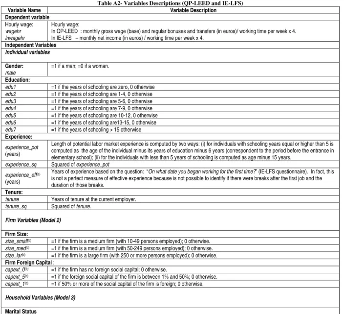
Table A2- Variables Descriptions (QP-LEED and IE-LFS)
Variable Name Variable Description
Dependent variable Hourly wage: wagehr lnwagehr
Hourly wage:
In QP-LEED : monthly gross wage (base) and regular bonuses and transfers (in euros)/ working time per week x 4. In IE-LFS – monthly net income (in euros) / working time per week x 4.
Independent Variables
Individual variables
Gender: male
=1 if a man; =0 if a woman.
Education:
edu1 =1 if the years of schooling are zero, 0 otherwise edu2 =1 if the years of schooling are 1-4, 0 otherwise edu3 =1 if the years of schooling are 5-6, 0 otherwise edu4 =1 if the years of schooling are 7-9, 0 otherwise edu5 =1 if the years of schooling are 10-12, 0 otherwise edu6 =1 if the years of schooling are13-15, 0 otherwise edu7 =1 if the years of schooling > 15 otherwise Experience:
experience_pot (years)
Length of potential labor market experience is computed by two ways: (i) for individuals with schooling years equal or higher than 5 is computed as the age of the individual minus its years of education minus 6 years (correspondent to the period before the entrance in elementary school); (ii) for the individuals with less than 5 years of schooling is computed as age minus 15 years.
experience_sq Squared of experience_pot experience_eff(a)
(years)
Years of experience based on the question: “On what date you began working for the first time?” (IE-LFS questionnaire). In fact, this is not a perfect measure of effective experience because is not possible to identify if there were breaks after the first job and the duration of those breaks.
Tenure:
tenure Years of tenure at the current employer. tenure_sq Squared of tenure.
Firm Variables (Model 2)
Firm Size:
size_small(b) =1 if the firm is a medium firm (with 10-49 persons employed); 0 otherwise.
size_med(b) =1 if the firm is a medium firm (with 50-249 persons employed); 0 otherwise.
size_lar(b) =1 if the firm is a large firm (with 250 or more persons employed); 0 otherwise.
Firm Foreign Capital :
capext_0(b) =1 if the firm has no foreign social capital; 0 otherwise.
capext_5(b) =1 if the foreign social capital of the firm is between 1% and 50%; 0 otherwise.
capext_1(b) =1 if 50% or more of the social capital of the firm is foreign; 0 otherwise.
Household Variables (Model 3)
Marital Status
married(a) =1 if the respondent is married or has a partner; 0 otherwise.
Children
Child <6(a) =1 if the respondent has at least a child less than 6 years old; 0 otherwise.
Child_6_17(a) =1 if the respondent has at least a child between 6 and 17 years old; 0 otherwise.
Child >17 (a) =1 if the respondent has a least a child >17 years old; 0 otherwise.
Sector
In QP-LEED: (note: the correspondence between sectors from the two data sources is not perfect; the Authors are working on the sector harmonization):
Binary variables: act1, Extractive except extracting energy products; act2, Manufacture of food, beverages and tobacco; act3, Textile industry;act4, Manufacture of leather and leather products;act5, Manufacture of wood and cork and articles thereof; act6, Industry of pulp, paper and paper products; publishing and printing;act7, Manufacture of coke, refined petroleum products and nuclear fuel;act8, Manufacture of chemicals and man-made fibers;act9, Manufacture of rubber and plastic products; act10, Manufacture of other non-metallic mineral products;act11, Manufacture of basic metals and fabricated metal products; act12, Manufacture of machinery and equipment, n. and.;act13, Manufacture of electrical and optical;act14, Manufacture of transport equipment; act15, Manufacturing, n. and.; act16, Production and distribution of electricity, gas and water; act17, Wholesale and retail trade, repair of motor vehicles, motorcycles and personal effects and household; act18, Hotels and restaurants; act19, Transport, storage and communications; act20, Financial activities [reference category]; act21, Real estate, renting and business services; act22, Other services, community, social and personal.
Occupation
In QP-LEED and IE-LFS:
Binary variables: occup1, senior staff; occup2, intellectual and scientific; occup3, technicians; occup4, clerks [reference category]; occup5, sellers and personal services; occup6, farmers and fishermen; occup7, craft and related jobs; occup8, machinery operators; occup9, unskilled.
23 Figure A.1. (1 to 41 ) – QR and OLS coefficients and confidence intervals for each regressor as q varies from 0 to 1
(male; education; experience; tenure; sector; job); Source: QP-LEED
Source: Authors computations based on QP-LEE 2007.
1. 2 0 1. 4 0 1. 6 0 1. 8 0 Int er cept
0 .2 .4 .6 .8 1 Quantile 0. 00 0. 1 0 0. 2 0 0. 30 0. 4 0 ma le
0 .2 .4 .6 .8 1 Quantile -0 .2 0-0 .1 00. 0 00. 1 00. 2 00. 3 0 ed 4
0 .2 .4 .6 .8 1 Quantile -0 .1 00. 00 0. 1 00. 2 00. 3 00. 4 0 ed 6
0 .2 .4 .6 .8 1 Quantile 0. 00 0. 10 0. 2 00. 3 00. 4 00. 5 0 ed 9
0 .2 .4 .6 .8 1 Quantile 0. 00 0. 2 0 0. 4 0 0. 60 0. 8 0 ed1 2
0 .2 .4 .6 .8 1 Quantile 0. 2 00. 4 00. 6 00. 8 01. 0 0 ed1 5
0 .2 .4 .6 .8 1 Quantile 0. 4 0 0. 6 0 0. 8 0 1. 0 0 1. 2 0 eds up
0 .2 .4 .6 .8 1 Quantile 0. 0 0 0. 0 1 0. 0 2 0. 0 3 0. 0 4 ex p er a
0 .2 .4 .6 .8 1 Quantile -0 .0 0 -0 .0 0 -0 .0 0 0. 0 0 ex p er aq
0 .2 .4 .6 .8 1 Quantile 0. 0 1 0. 0 1 0. 0 1 0. 0 2 0. 03 te n u re
0 .2 .4 .6 .8 1 Quantile -0 .0 0 -0 .0 0 -0 .0 0 0. 0 0 tenu res q
0 .2 .4 .6 .8 1 Quantile -0 .8 0-0 .6 0-0 .4 0-0 .2 0 0. 0 0 s0 1
0 .2 .4 .6 .8 1 Quantile -0 .8 0-0 .6 0-0 .4 0-0 .2 0 0. 0 0 s0 2
0 .2 .4 .6 .8 1 Quantile -0 .9 0-0 .8 0-0 .7 0-0 .6 0-0 .5 0 s0 3
0 .2 .4 .6 .8 1 Quantile -0 .9 0-0 .8 0-0 .7 0-0 .6 0-0 .5 0 s0 4
0 .2 .4 .6 .8 1 Quantile -0 .8 0-0 .6 0-0 .4 0-0 .2 00. 0 0 s0 5
0 .2 .4 .6 .8 1 Quantile -1 .0 0-0 .8 0-0 .6 0-0 .4 0-0 .2 0 s0 6
0 .2 .4 .6 .8 1 Quantile -1 .5 0-1 .0 0-0 .5 00. 00 0. 50 1. 0 0 s0 7
0 .2 .4 .6 .8 1 Quantile -1 .0 0 -0 .5 0 0. 0 0 0. 5 0 s0 8
0 .2 .4 .6 .8 1 Quantile -0 .8 0-0 .6 0-0 .4 0-0 .2 00. 0 0 s0 9
0 .2 .4 .6 .8 1 Quantile -0 .8 0-0 .6 0-0 .4 0-0 .2 0 0. 00 s1 0
0 .2 .4 .6 .8 1 Quantile -0 .8 0 -0 .6 0 -0 .4 0 -0 .2 0 s1 1
0 .2 .4 .6 .8 1 Quantile -0 .8 0-0 .6 0-0 .4 0-0 .2 0 0. 00 s1 2
0 .2 .4 .6 .8 1 Quantile -0 .6 0 -0 .4 0 -0 .2 0 0. 00 s1 3
0 .2 .4 .6 .8 1 Quantile -0 .7 0-0 .6 0-0 .5 0-0 .4 0-0 .3 0-0 .2 0 s1 4
0 .2 .4 .6 .8 1 Quantile -1 .0 0-0 .8 0-0 .6 0-0 .4 0-0 .2 0 s1 5
0 .2 .4 .6 .8 1 Quantile -0 .6 0-0 .4 0-0 .2 00. 0 00. 20 0. 40 s1 6
0 .2 .4 .6 .8 1 Quantile -0 .8 0 -0 .6 0 -0 .4 0 -0 .2 0 s1 7
0 .2 .4 .6 .8 1 Quantile -0 .8 0 -0 .6 0 -0 .4 0 -0 .2 0 s1 8
0 .2 .4 .6 .8 1 Quantile -0 .6 0 -0 .4 0 -0 .2 0 0. 0 0 s1 9
0 .2 .4 .6 .8 1 Quantile -0 .7 0-0 .6 0-0 .5 0-0 .4 0-0 .3 0-0 .2 0 s2 1
0 .2 .4 .6 .8 1 Quantile -0 .8 0-0 .6 0-0 .4 0-0 .2 0 0. 0 0 s2 2
0 .2 .4 .6 .8 1 Quantile 0. 0 0 0. 5 0 1. 0 0 1. 5 0 js kll
0 .2 .4 .6 .8 1 Quantile 0. 2 00. 30 0. 4 00. 5 00. 6 00. 7 0 js ci
0 .2 .4 .6 .8 1 Quantile 0. 0 0 0. 1 0 0. 2 0 0. 30 0. 40 jt e c
0 .2 .4 .6 .8 1 Quantile -0 .3 0 -0 .2 0 -0 .1 0 0. 0 0 js rv
0 .2 .4 .6 .8 1 Quantile -1 .0 0 -0 .5 0 0. 0 0 0. 5 0 jagr
0 .2 .4 .6 .8 1 Quantile -0 .4 0-0 .3 0-0 .2 0-0 .1 00. 00 jb lu e
0 .2 .4 .6 .8 1 Quantile -0 .3 0 -0 .2 0 -0 .1 0 0. 00 jm w
0 .2 .4 .6 .8 1 Quantile -0 .5 0-0 .4 0-0 .3 0-0 .2 0-0 .1 00. 0 0 jn s k
24
Figure A.1. (1 to 39 ) – QR and OLS coefficients and confidence intervals for each regressor as q varies from 0 to 1 (male; education; experience; tenure; sector; job); Source: IE-LFS
Source: Authors computations based on IE-LFS 2007.
0. 60 0. 8 01. 00 1. 20 1. 4 0 Int er cept
0 .2 .4 .6 .8 1 Quantile Fig. A2.1 const.
0. 10 0. 15 0. 20 0. 2 50. 30 se xo
0 .2 .4 .6 .8 1 Quantile Fig. A2.2 male
-0 .1 00. 0 00. 10 0. 20 0. 3 0 ni v _c or r= 2. 000 0
0 .2 .4 .6 .8 1 Quantile Fig. A2. 3 edu02
0. 00 0. 1 00. 20 0. 3 00. 4 0 ni v _c or r= 3. 000 0
0 .2 .4 .6 .8 1 Quantile Fig. A2. 4 edu03
0. 000. 10 0. 200. 30 0. 400. 5 0 ni v _c or r= 4. 000 0
0 .2 .4 .6 .8 1 Quantile Fig. A2 5 edu04
0. 1 00. 2 00. 3 00. 4 00. 5 00. 6 0 ni v _c or r= 5. 000 0
0 .2 .4 .6 .8 1 Quantile Fig. A2 6 edu05
0. 2 00. 4 00. 60 0. 80 1. 00 ni v _c or r= 6. 000 0
0 .2 .4 .6 .8 1 Quantile Fig. A2 7 edu06
0. 2 00. 4 00. 6 00. 8 01. 0 01. 2 0 ni v _c o rr = 7. 0000
0 .2 .4 .6 .8 1 Quantile Fig. A2 8 edu07
0. 0 1 0. 0 2 0. 0 3 0. 0 4 ex p _pot
0 .2 .4 .6 .8 1 Quantile Fig. A2 9 experience pot
-0 .0 0 -0 .0 0 -0 .0 0 0. 0 0 e x p_po t2
0 .2 .4 .6 .8 1 Quantile Fig. A2 10 experience^2
0. 0 0 0. 0 1 0. 0 1 0. 0 1 0. 0 2 an ti g
0 .2 .4 .6 .8 1 Quantile Fig. A2 11 tenure
-0 .0 0 -0 .0 0 0. 0 0 0. 0 0 an ti g 2
0 .2 .4 .6 .8 1 Quantile Fig A2 12 tenure^2
-0 .6 0-0 .4 0-0 .2 0 0. 0 0 0. 2 0 g_ac t= 1. 0 000
0 .2 .4 .6 .8 1 Quantile Fig. A2 13 mining
-0 .6 0-0 .5 0-0 .4 0-0 .3 0-0 .2 0 g_ac t= 2. 0 000
0 .2 .4 .6 .8 1 Quantile Fig. A2 14 food & tab
-0 .6 0 -0 .5 0 -0 .4 0 -0 .3 0 -0 .2 0 g_ a c t= 3 .00 00
0 .2 .4 .6 .8 1 Quantile Fig. A2 15 textile & leader
-0 .6 0-0 .5 0-0 .4 0-0 .3 0-0 .2 0 g_ a c t= 4 .00 00
0 .2 .4 .6 .8 1 Quantile Fig. A2 16 wood & cork
-0 .5 0-0 .4 0-0 .3 0-0 .2 0-0 .1 0 g_ac t= 5. 0 000
0 .2 .4 .6 .8 1 Quantile Fig. A2 17 paper
-0 .6 0-0 .4 0-0 .2 0 0. 0 0 0. 2 0 g_ac t= 6. 0 000
0 .2 .4 .6 .8 1 Quantile Fig. A2 18 chemicals
-0 .6 0-0 .5 0-0 .4 0-0 .3 0-0 .2 0-0 .1 0 g_ a c t= 7 .00 00
0 .2 .4 .6 .8 1 Quantile Fig. A2 19 min non met
-0 .6 0-0 .5 0-0 .4 0-0 .3 0-0 .2 0-0 .1 0 g_ac t= 8. 0 000
0 .2 .4 .6 .8 1 Quantile Fig. A2 20 basic metals
-0 .5 0-0 .4 0-0 .3 0-0 .2 0-0 .1 0 g_ac t= 9. 0 000
0 .2 .4 .6 .8 1 Quantile Fig. A2 21 machinery
-0 .6 0-0 .5 0-0 .4 0-0 .3 0-0 .2 0-0 .1 0 g_ ac t= 1 0. 0 0 0 0
0 .2 .4 .6 .8 1 Quantile Fig. A2 22 other manufact.
-0 .4 0-0 .2 00. 0 0 0. 2 0 0. 4 0 g_ ac t= 1 1. 0 0 0 0
0 .2 .4 .6 .8 1 Quantile Fig. A2 23 elect.gas water
-0 .6 0-0 .5 0-0 .4 0-0 .3 0-0 .2 0 g_ac t= 13. 000 0
0 .2 .4 .6 .8 1 Quantile Fig. A2 24 retail tr
-0 .5 0-0 .40-0 .3 0-0 .20-0 .1 00. 0 0 g_ac t= 14. 000 0
0 .2 .4 .6 .8 1 Quantile Fig. A2 25 wholesale t
-0 .6 0-0 .5 0-0 .4 0-0 .3 0-0 .2 0 g_ac t= 15. 000 0
0 .2 .4 .6 .8 1 Quantile Fig. A2 26 hospitality
-0 .4 0-0 .3 0-0 .20-0 .1 00. 000. 1 0 g _ac t161 7
0 .2 .4 .6 .8 1 Quantile Fig. A2 27 transports
-0 .6 0-0 .5 0-0 .40-0 .3 0-0 .20-0 .1 0 g_ac t= 20. 000 0
0 .2 .4 .6 .8 1 Quantile Fig. A2 28 real estate
-0 .5 0-0 .40-0 .30-0 .20-0 .1 00. 0 0 g _ac t= 21. 0000
0 .2 .4 .6 .8 1 Quantile Fig. A2 29 sanit serv
-0 .6 0-0 .4 0-0 .2 00. 00 0. 2 0 g _ac t= 22. 0000
0 .2 .4 .6 .8 1 Quantile Fig. A2 30 assoc
-0 .6 0-0 .4 0-0 .2 00. 0 00. 2 0 g _ac t= 23. 0000
0 .2 .4 .6 .8 1 Quantile Fig. A2 31 cultural serv
-0 .2 00. 000. 20 0. 400. 6 00. 8 0 g _pr of = 1. 0000
0 .2 .4 .6 .8 1 Quantile Fig. A2 32 senior staff
0. 0 00. 1 00. 2 00. 3 00. 4 00. 5 0 g _ pr o f= 2 .00 00
0 .2 .4 .6 .8 1 Quantile Fig. A2 33 intellect.&sci
0. 00 0. 1 00. 2 00. 30 0. 40 g _pr of = 3. 0000
0 .2 .4 .6 .8 1 Quantile Fig. A2 34 technicians
-0 .2 0-0 .1 5-0 .1 0-0 .0 50. 00 g _pr of = 5. 0000
0 .2 .4 .6 .8 1 Quantile Fig. A2 35 sellers & serv
-0 .6 0-0 .4 0-0 .2 00. 0 00. 20 g_ pr o f= 6. 0 000
0 .2 .4 .6 .8 1 Quantile Fig. A2 36 farmers
-0 .3 0-0 .2 0-0 .1 00. 00 g_ pr o f= 7. 0 000
0 .2 .4 .6 .8 1 Quantile Fig A2 37 laborers
-0 .3 0-0 .2 0-0 .1 00. 0 00. 10 g_ pr o f= 8. 0 000
0 .2 .4 .6 .8 1 Quantile Fig. A2 38 operators
-0 .3 0-0 .2 0-0 .1 00. 00 g_ pr o f= 9. 0 000