www.atmos-chem-phys.net/15/1087/2015/ doi:10.5194/acp-15-1087-2015
© Author(s) 2015. CC Attribution 3.0 License.
A regional carbon data assimilation system and its preliminary
evaluation in East Asia
Z. Peng1, M. Zhang2, X. Kou2,3, X. Tian4, and X. Ma4
1School of Atmospheric Sciences, Nanjing University, Nanjing 210093, China
2State Key Laboratory of Atmospheric Boundary Layer Physics and Atmospheric Chemistry, Institute of Atmospheric
Physics, Chinese Academy of Sciences, Beijing 100029, China
3Graduate School of Chinese Academy of Sciences, University of Chinese Academy of Sciences, Beijing 100049, China 4Institute of Atmospheric Physics, Chinese Academy of Sciences, Beijing 100029, China
Correspondence to:Z. Peng ([email protected]) and M. Zhang ([email protected])
Received: 21 June 2014 – Published in Atmos. Chem. Phys. Discuss.: 8 August 2014 Revised: 15 November 2014 – Accepted: 29 December 2014 – Published: 30 January 2015
Abstract. In order to optimize surface CO2 fluxes at grid
scales, a regional surface CO2flux inversion system (Carbon
Flux Inversion system and Community Multi-scale Air Qual-ity, CFI-CMAQ) has been developed by applying the ensem-ble Kalman filter (EnKF) to constrain the CO2
concentra-tions and applying the ensemble Kalman smoother (EnKS) to optimize the surface CO2fluxes. The smoothing operator
is associated with the atmospheric transport model to con-stitute a persistence dynamical model to forecast the surface CO2flux scaling factors. In this implementation, the
“signal-to-noise” problem can be avoided; plus, any useful observed information achieved by the current assimilation cycle can be transferred into the next assimilation cycle. Thus, the sur-face CO2fluxes can be optimized as a whole at the grid scale
in CFI-CMAQ. The performance of CFI-CMAQ was quan-titatively evaluated through a set of Observing System Sim-ulation Experiments (OSSEs) by assimilating CO2retrievals
from GOSAT (Greenhouse Gases Observing Satellite). The results showed that the CO2concentration assimilation
us-ing EnKF could constrain the CO2concentration effectively,
illustrating that the simultaneous assimilation of CO2
con-centrations can provide convincing CO2initial analysis fields
for CO2flux inversion. In addition, the CO2flux optimization
using EnKS demonstrated that CFI-CMAQ could, in general, reproduce true fluxes at grid scales with acceptable bias. Two further sets of numerical experiments were conducted to in-vestigate the sensitivities of the inflation factor of scaling fac-tors and the smoother window. The results showed that the ability of CFI-CMAQ to optimize CO2fluxes greatly relied
on the choice of the inflation factor. However, the smoother window had a slight influence on the optimized results. CFI-CMAQ performed very well even with a short lag-window (e.g. 3 days).
1 Introduction
Considerable progress has been made in recent years to re-duce the uncertainties of surface CO2flux estimates through
the use of an advanced data assimilation technique (e.g. Chevallier, 2007; Chevallier et al., 2005, 2007; Baker et al., 2006; Engelen et al., 2009; Liu et al., 2012). Feng et al. (2009) showed that the uncertainties of surface CO2flux
estimates can be reduced significantly by assimilating OCO XCO2 measurements. Peters et al. (2005, 2007, 2009) devel-oped a surface CO2flux inversion system, CarbonTracker, by
incorporating the ensemble square-root filter (EnSRF) into the atmospheric transport TM5 model; the inversion results obtained by assimilating in situ surface CO2observations are
in excellent agreement with a wide collection of carbon in-ventories that form the basis of the first North American State of the Carbon Cycle Report (SOCCR) (Peters et al., 2007). CarbonTracker has also been frequently used to constrain the surface CO2fluxes over Europe and Asia (eg., Zhang et al.,
2014a, b). Kang et al. (2012) presented a simultaneous data assimilation of surface CO2fluxes and atmospheric CO2
that an accurate estimation of the evolving surface fluxes can be gained even without any a priori information. Recently, Tian et al. (2014) developed a new surface CO2 flux data
assimilation system, Tan-Tracker, by incorporating a joint PODEn4DVar assimilation framework into the GEOS-Chem model on the basis of Peters et al. (2005, 2007) and Kang et al. (2011, 2012). They discussed in detail that the assimi-lation of CO2surface fluxes could be improved through the
use of simultaneous assimilation of CO2concentrations and
CO2 surface fluxes. Despite the rigour of data assimilation
theory, current CO2 flux-inversion methods still face many
challenging scientific problems, such as: (1) the well-known “signal-to-noise” problem (NRC, 2010); (2) large inaccura-cies in chemical transport models (e.g. Prather et al., 2008); (3) vast computational expenses (e.g. Feng et al., 2009); and (4) the sparseness of observation data (e.g. Gurney et al., 2002).
The “signal-to-noise” problem is one of the most challeng-ing issues for an ensemble-based CO2flux inversion system
due to the fact that surface CO2fluxes are the model forcing
(or boundary condition), rather than model states (like CO2
concentrations), of the chemistry transport model (CTM). In the absence of a suitable dynamical model to describe the evolution of the surface CO2fluxes, most CO2flux-inversion
studies have traditionally ignored the uncertainty of anthro-pogenic and other CO2 emissions and focused on the
opti-mization of natural (i.e. biospheric and oceanic) CO2
emis-sions at the ecological scale (e.g. Deng et al., 2007; Feng et al., 2009; Peters et al., 2005, 2007; Jiang et al., 2013; Peylin et al., 2013).
This compromise is acceptable to some extent. Indeed, the total amount of anthropogenic CO2 emissions can
be estimated by relatively well-documented global fuel-consumption data with a small degree of uncertainty (Bo-den et al., 2011), and the uncertainties involved in the total amount of anthropogenic CO2 emissions are much smaller
than those related to natural emissions. However, their spatial distribution, strength and temporal development still remain elusive because of their inherent non-uniformities (Andres et al., 2012; Gurney et al., 2009). Marland (2008) pointed out that even a tiny amount of uncertainty, i.e. 0.9 %, in one of the leading emitter countries like the U.S. is equivalent to the total emissions of the smaller emitter countries in the world. Furthermore, the usual values of anthropogenic CO2
emis-sions in chemical transport models have thus far been sim-ply interpolated from very coarse monthly-mean fuel con-sumption data. Therefore, great uncertainty in the spatiotem-poral distributions of anthropogenic emissions likely exists, which could reduce the accuracy of CO2concentration
sim-ulations and subsequently increase the inaccuracy of natural CO2flux inversion results. In addition, current research
ap-proaches tend only to assimilate natural CO2emissions at the
ecological scale, which is far from sufficient. Therefore, sur-face CO2fluxes should be constrained as a whole at a finer
scale.
In CarbonTracker (Peters at al., 2007), a smoothing opera-tor is innovatively applied as the persistence forecast model. In that application, the surface CO2fluxes can be treated as
the model states and the observed information ingested by the current assimilation cycle can be used in the next as-similation cycle effectively. However, the “signal-to-noise” problem has not yet been resolved, and thus CarbonTracker also has to assimilate natural CO2emissions at the
ecolog-ical scale only. In Tan-Tracker (Tian et al., 2014), a four-dimensional (4-D) moving sampling strategy (Wang et al., 2010) is used to generate the flux ensemble members, and so the surface CO2 fluxes can be optimized as a whole at
the grid scale. In this work, the persistence dynamical model taken by Peters et al. (2005) was further developed for the purpose of resolving the “signal-to-noise” problem, to opti-mize the surface CO2fluxes as a whole at the grid scale. This
process is described in detail in Sect. 2 of this paper. The surface CO2 flux inversion system presented in this
paper was developed by simultaneously optimizing the sur-face CO2 fluxes and constraining the CO2 concentrations.
As we know, assimilating CO2 observations from multiple
sources can improve the accuracy of simulation results (e.g. Miyazaki, 2009; Liu et al., 2011, 2012; Feng et al., 2011; Tangborn et al., 2013; Huang et al., 2014). In addition, pre-vious studies showed that the simultaneous assimilation of CO2concentrations and surface CO2fluxes can largely
elim-inate the uncertainty in initial CO2concentrations on the CO2
evolution (Kang et al., 2012; Tian et al., 2014). Therefore, we also use the simultaneous assimilation framework; the ensemble Kalman filter (EnKF) was used to constrain CO2
concentrations and the ensemble Kalman smoother (EnKS) was used to optimize surface CO2fluxes. Since the regional
chemical transport models, compared to global models, have some advantages in reproducing the effects of meso–micro– scale transport on atmospheric CO2distributions (Ahmadov
et al., 2009; Pillai et al., 2011; Kretschmer et al., 2012), we choose a regional model, Regional Atmospheric Modeling System and Community Multi-scale Air Quality (RAMS-CMAQ) (Zhang et al., 2002, 2003, 2007; Kou et al., 2013; Liu et al., 2013; Huang et al., 2014), to develop this in-version system. For simplicity, this system is referred to as CFI-CMAQ (Carbon Flux Inversion system and Community Multi-scale Air Quality).
Since this is the first introduction of CFI-CMAQ, we focus mainly on introducing the methodology in this paper. Nev-ertheless, in addition, Observing System Simulation Experi-ments (OSSEs) were designed to assess the system’s ability to optimize surface CO2fluxes. The retrieval information of
GOSAT XCO2 are used to generate artificial observations be-cause of the sparseness and heterogeneity of ground-based measurements.
The remainder of the paper is organized as follows. Sec-tion 2 describes the details of the regional surface CO2flux
EnKF assimilation approaches, and the process involved. The experimental designs are then introduced and the assim-ilation results shown in Sect. 3. Finally, a summary and con-clusions are provided in Sect. 4.
2 Framework of the regional surface CO2flux
inversion system
Suppose we have the prescribed net CO2 surface flux, F∗(x, y, z, t ), which can be released from a climate model or be generated by other’s methods, our ultimate goal is to op-timizeF∗(x, y, z, t )by assimilating CO2observations from
various platforms. As an ensemble-based assimilation sys-tem, CFI-CMAQ was also developed by applying a set of lin-ear multiplication factors, similar to the approach by Peters et al. (2007) and Tian et al. (2014). Theith ensemble mem-ber of the surface fluxes,Fi(x, y, z, t ), from anN-member ensemble can be described by
Fi(x, y, z, t )=λi(x, y, z, t )F∗(x, y, z, t ), (i=1, . . ., N ), (1) whereλi(x, y, z, t )represents the ith ensemble member of the linear scaling factors (Peters et al., 2007; Tian et al., 2014) for each time and each grid to be optimized in the as-similation. The notations are standard: the subscriptirefers to the ith ensemble member. In the following,λi(x, y, z, t ) is referred to as λi,t,F∗(x, y, z, t )is referred to as F∗t, and Fi(x, y, z, t )is referred to asFi,t for simplicity.
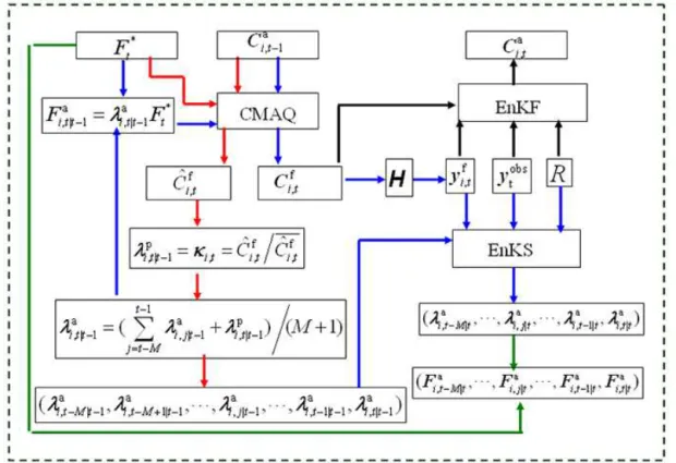
At each optimization cycle, CFI-CMAQ includes the following four parts in turn (see Fig. 1): (1) forecasting of the linear scaling factors at time t,
λai,t|t−1; (2) optimization of the scaling factors in the smoother window, (λai,t−M|t−1,λai,t−M+1|t−1, . . .,
λai,j|t−1, . . .,λai,t−1|t−1,λai,t1|t−1), by EnKS, where
λai,j|t−1(j=t−1−M, . . ., t−1) refer to analysed quan-tities from the previous assimilation cycle at time j (see Fig. 1), |t−1 means that these factors have been updated using observations before time t−1, and the super-script a refers to the analysed; (3) updating of the fluxes in the smoother window, (Fai,t−M|t−1,Fai,t−M+1|t−1, . . ., Fai,j|t−1, . . .,Fai,t−1|t−1,Fai,t|t−1); and (4) assimilation of the forecast CO2 concentration fields at time t, Cif(x, y, z, t )
(referred to as Cfi,t, and the superscript f refers to the forecast or the background), by EnKF. A flowchart illus-trating CFI-CMAQ is presented in Fig. 2. The assimilation procedure is addressed in detail below. In addition, the observation operator is introduced, particularly for use in the GOSAT XCO2 data in Sect. 2.4. Furthermore, covariance inflation and localization techniques applied in CFI-CMAQ are introduced briefly in Sect. 2.5.
2.1 Forecasting the linear scaling factors at timet λai,t|t−1
In the previous assimilation cycle t−1−M∼t−1 (see Fig. 1), the optimized scaling factors in the smoother window are (λai,t−1−M|t−1, λai,t−M|t−1,λai,t−M+1|t−1, . . .,
λai,j|t−1, . . .,λi,ta −1|t−1) and the assimilated CO2
con-centration fields at time t−1 are Cia(x, y, z, t−1) (referred to as Cai,t−1). In the current assimilation cycle t−M∼t, the scaling factors in the current smoother window are (λai,t−M|t−1,λai,t−M+1|t−1, . . .,λai,j|t−1, . . .,
λai,t−1|t−1,λai,t|t−1) and the forecast CO2concentration fields
at timetareCfi,t.
In order to pass the useful observed information onto the next assimilation cycle effectively, following Peters et al. (2007) the smoothing operator is applied as part of the persistence dynamical model to calculate the linear scaling factorsλai,t|t−1,
λai,t|t−1=
( t−1
P
j=t−M
λai,j|t−1+λpi,t|t−1)
M+1 , (i=1, . . ., N ), (2) whereλpi,t|t−1refers to the prior values of the linear scaling factors at timet. The superscriptprefers to the prior. This operation represents a smoothing over all the time steps in the smoother window (see Fig. 1), thus dampening variations in the forecast ofλai,t|t−1in time.
In order to generate λpi,t|t−1, the atmospheric transport model (CMAQ) is applied and a set of ensemble forecast ex-periments are carried out. It integrates from timet−1 totto produce the CO2concentration fieldsCˆif(x, y, z, t )(referred to asCˆi,tf hereafter to distinguish fromCfi,t)forced by the prescribed net CO2surface fluxF∗t withCai,t−1as initial
con-ditions. Then, the ratioκi,t= ˆCi,tf .Cˆi,tf is calculated, where
ˆ
Ci,tf =N1
N
P
i=1
ˆ
Ci,tf . Suppose thatλpi,t|t−1=κi,t due to the fact that the surface CO2fluxes correlate with its concentrations,
the values forλpi,t|t−1are obtained and thenλai,t|t−1 can fi-nally be calculated (see the red arrows in the flowchart in Fig. 2).
The way the prior scaling factorλpi,t|t−1is updated by as-sociating with the atmospheric transport model is the main improvement over the one used in CarbonTracker (Peters et al., 2007). In CarbonTracker, allλpi,t|t−1are set to 1 (Peters et al., 2007). The distribution of the ensemble members of the linear scaling factors at timet,λpi,t|t−1, are finally depen-dent on the distribution of the previous scaling factors be-cause Eq. (2) is a linear smoothing operator. In this study, the values ofλpi,t|t−1are updated by association with the atmo-spheric transport model. It is important to note thatλpi,t|t−1
Figure 1.Schematic diagram of the smoother window.(λa
i,t−1−M|t−1, λai,t−M|t−1,λai,t−M+1|t−1, . . .,λai,j|t−1, . . .,λai,t−1|t−1)are the
op-timized scaling factors in the smoother window and Cai,t−1are the assimilated CO2concentrations fields at timet−1 in the previous
assimilation cyclet−1−M∼t−1.(λa
i,t−M|t−1,λai,t−M+1|t−1, . . .,λai,j|t−1, . . .,λai,t−1|t−1,λai,t|t−1)are the scaling factors in the smoother
window andCfi,t are the forecast CO2concentrations fields at timetwhich need to be optimized in the current assimilation cyclet−M∼ t.
Figure 2.Flowchart of the CFI-CMAQ system used to optimize surface CO2fluxes at each assimilation cycle. The system includes the
following four parts in turn: (1) forecasting of the linear scaling factorsλa
i,t|t−1(red arrows); (2) optimization of the scaling factors in the
smoother window by EnKS (see Fig. 1) (blue arrows); (3) updating of the flux in the smoother window (green arrows); and (4) assimilation of the CO2concentration fields at timetby EnKF (black arrows).
the scaling factors in the smoother window. An OSSE was designed to illustrate the difference between our method and the one in whichλpi,t|t−1are set to 1 in Sect. 3.
It is also important to note that, similar to Peters et al. (2007), this dynamical model equation still does not
2.2 Optimizing the scaling factors in the smoother window by EnKS
Substitutingλai,t|t−1into Eq. (1), theith member of the sur-face fluxes at timet,Fai,t|t−1, can be generated. Then, forced byFai,t|t−1, CMAQ was run from timet−1 tot to produce the background concentration fieldCfi,t withCai,t−1as initial conditions.
In the current assimilation cycle t−M∼t (see Fig. 1), the scaling factors to be optimized in the smoother window are (λai,t−M|t−1,λai,t−M+1|t−1, . . .,λai,j|t−1, . . .,
λai,t−1|t−1,λai,t|t−1), as stated in the first paragraph of Sect. 2.1. Using the EnKS analysis technique, these scaling factors are updated in turn via
λai,j|t=λai,j|t−1+Kj,te |t−1(ytobs−yfi,t+υi,t),
(i=1, . . ., N, j =t−M, . . ., t ), (3)
Kej,t|t−1=Sej,t|t−1HT(HSet,t|t−1HT +R)−1, (4) Sej,t|t−1= 1
N−1 N X
i=1 [λa
i,j|t−1−λai,j|t−1][λai,t|t−1−λai,t|t−1]T, (5) Set,t|t−1= 1
N−1 N X
i=1
[λai,t|t−1−λa i,t|t−1][λ
a
i,t|t−1−λai,t|t−1]
T, (6)
yfi,t =H (φt−1→t(λai,t|t−1))=H (C f
i,t), (7)
whereKej,t|t−1 is the Kalman gain matrix of EnKS,yobst is the observation vector measured at timetandyfi,t is the sim-ulated values, υi,t is a random normal distribution pertur-bation field with zero mean, Sej,t|t−1 is the background er-ror cross-covariance between the state vector λai,j|t−1 and
λai,t|t−1, Set,t|t−1 is the background error covariance of the state vector λai,t|t−1, H (·) is the observation operator that maps the state variable from model space into observation space,Ris the standard deviation representing the measure-ment errors, andφ (·)is the atmospheric transport model.
In actual implementations, it is unnecessary to calculate Sej,t|t−1andSet,t|t−1separately.Sj,te |t−1HT andHSet,t|t−1HT can be calculated as a whole by
Sej,t|t−1HT = 1 N−1
N X
i=1 [λa
i,j|t−1−λai,j|t−1][y f
i,t−yft]T, (8)
HSet,t|t−1HT = 1
N−1 N
X
i=1
[yfi,t−yft][yfi,t−yft]T, (9)
yft=H (Cft)=H (1 N
N
X
i=1
Cfi,t). (10)
After EnKS, (λai,t−M|t,λi,ta −M+1|t, . . .,λai,j|t, . . . ,λai,t−1|t,λai,t|t) are gained. Then the corre-sponding fluxes in the smoother window (Fai,t−M|t,Fai,t−M+1|t, . . .,Fai,j|t, . . .,Fai,t−1|t,Fai,t|t)
can be gained (see the green arrows in the flowchart in Fig. 2) by substituting (λai,t−M|t,λai,t−M+1|t, . . .,λai,j|t, . . .,λai,t−1|t,λai,t|t) into Eq. (1).
Then the ensemble mean values of the assimilated fluxes in the smoother window can be calculated via,
Fai,j|t = 1
N N
X
i=1
Fai,j|t, (j=t−M, . . ., t ). (11)
Finally, those ensemble mean assimilated fluxes which are before the next smoother window and will not be updated by the succeeding observations are regarded as the final op-timized fluxes. We referred to them asFat for simplicity. 2.3 Assimilating the CO2concentration fields at timet
by EnKF
The analysis of CO2 concentrations fields at time t in the
EnKF scheme is updated via
Cai,t =Cfi,t+K(yobst −yft+υi,t), (12) K=PfHT(HPfHT +R)−1, (13) whereKis the Kalman gain matrix of EnKF,Pfis the back-ground error covariance among the backback-ground CO2
concen-tration fieldsCfi,t.
In the actual application,PfHT andHPfHT can be calcu-lated as a whole by
PfHT = 1
N−1 N
X
i=1
[Cfi,t−Cft][yfi,t−yft]T, (14)
HPfHT = 1
N−1 N
X
i=1
[yfi,t−yft]T[yfi,t−yft]T, (15)
Cft = 1
N N
X
i=1
Cfi,t. (16)
Finally, the ensemble mean values of the assimilated CO2
concentrations fields can be gained via
Cat = 1
N N
X
i=1
Cai,t, (17)
whereCat is regarded as the final analysing concentration field.
2.4 The observation operator
XCO2 should be calculated with the same weighted column average method (Connor et al., 2008; Crisp et al., 2010, 2012; O’Dell et al., 2012). Hence, the observation operator to as-similate the GOSAT XCO2 retrieval is
yfi,t =H (φt−1→t(λai,t|t−1))=H (Cfi,t)=ypriori
+hTaCO2(S(C
f i,t)−f
priori),
(18) whereyfi,t is the simulated XCO2;y
priori is the a priori CO 2
column average used in the GOSAT XCO2 retrieval process; S(·)is the spatial bilinear interpolation operator that inter-polates the simulated fields to the GOSAT XCO2 locations to obtain the simulated CO2vertical profiles there;fprioriis the
a priori CO2vertical profile used in the retrieval process;h
is the pressure weighting function, which indicates the con-tribution of the retrieved value from each layer of the atmo-sphere; andaCO2 is the normalized averaging kernel. 2.5 Covariance inflation and localization
In order to keep the ensemble spread of the CO2
concentra-tions at a certain level and compensate for transport model error to prevent filter divergence, covariance inflation is ap-plied before updating the CO2concentrations. So,
(Cfi,t)new=α(Cfi,t−Cfi,t)+Cfi,t, (19) where α is the inflation factor of CO2 concentrations and (Cfi,t)newis the final field used for data assimilation.
Similarly, covariance inflation is also used to keep the en-semble spread of the prior scaling factors at a certain level and compensate for dynamical model error. Hence,
(λpi,t|t−1)new=β(λpi,t|t−1−λ p
i,t|t−1)+λ p
i,t|t−1, (20)
where β is the inflation factor of scaling factors and (λpi,t|t−1)newis the final scaling factors used for data
assimi-lation.
In addition, the Schur product is utilized to filter the remote correlation resulting from the spurious long-range correlations (Houtekamer and Mitchell 2001). Hence, the Kalman gain matrixKej,t|t−1andKare updated via
Kej,t|t−1= [(ρ◦Sej,t|t−1)HT(H (ρ◦Pet,t|t−1)HT+R)−1, (21) K= [(ρ◦Pf)HT][(H (ρ◦Pf)HT +R]−1, (22) where the filtering matrixρis calculated using the formula
C0(r, c)= −1 4 |r|
c 5
+1
2
|r|
c 4
+5
8
|r|
c 3
−5
3
|r|
c 2
+1,0≤ |r| ≤c 1 12 | r| c 5 −1 2 | r| c 4 +5 8 | r| c 3 + 5 3 | r| c 2 −5 | r| c +4−2
3
c |r|
, c≤ |r| ≤2c
0, c≤ |r| ,
(23)
wherecis the element of the localization Schur radius. The matrixρ can filter the small background error correlations associated with remote observations through the Schur prod-uct (Tian et al., 2011); and the Schur prodprod-uct tends to reduce the effect of those observations smoothly at intermediate dis-tances due to the smooth and monotonically decreasing of the filtering matrix.
3 OSSEs for evaluation of CFI-CMAQ
A set of OSSEs were designed to quantitatively assess the performance of CFI-CMAQ. The setup of the experiments and the results are described in this section.
3.1 Experimental setup
The chemical transport model utilized was RAMS-CMAQ (Zhang et al., 2002), in which CO2 was treated as an
in-ert tracer. The model domain was 6654×5440 km2on a ro-tated polar stereographic map projection centred at (35.0◦N, 116.0◦E), with a horizontal grid resolution of 64× 64 km2 and 15 vertical layers in theσz-coordinate system, unequally spaced from the surface to approximately 23 km. The ini-tial fields and boundary conditions of the CO2
concentra-tions were interpolated from the simulated CO2 fields of
CarbonTracker 2011 (Peters et al., 2007). The prior sur-face CO2fluxes included biosphere–atmosphere CO2fluxes,
ocean–atmosphere CO2 fluxes, anthropogenic emissions,
and biomass-burning emissions (Kou et al., 2013), Fp(x, y, z, t )=Fbio(x, y, z, t )+Foce(x, y, z, t )
+Fff(x, y, z, t )+Ffire(x, y, z, t ), (24)
whereFp(x, y, z, t ) (referred to as Fpt) was the prior sur-face CO2 flux; Fbio(x, y, z, t ) and Foce(x, y, z, t ) were the
biosphere–atmosphere and ocean–atmosphere CO2 fluxes,
respectively, which were obtained from the optimized results of CarbonTracker 2011 (Peters et al., 2007); Fff(x, y, z, t )
was fossil fuel emissions, adopted from the Regional Emis-sion inventory in ASia (REAS, 2005 Asia monthly mean emission inventory) with a spatial resolution of 0.5◦×0.5◦ (Ohara et al., 2007); and Ffire(x, y, z, t ) was biomass–
burning emissions, provided by the monthly mean inven-tory at a spatial resolution of 0.5◦×0.5◦ from the Global Fire Emissions Database, Version 3 (GFED v3) (van der Werf et al., 2010). Among all these fluxes, Fbio(x, y, z, t ), Foce(x, y, z, t )andFff(x, y, z, t )had nonzero values at model
level 1, while they all were zeros at the other 14 levels. How-ever,Ffire(x, y, z, t )had nonzero values at model level 1∼5
and they were all zeros at other the 10 levels. So, all fluxes in this paper were the function of(x, y, z, t )for convenience.
Firstly, the prior fluxFpt was assumed as the true surface CO2 flux in all of the following OSSEs. Forced byF
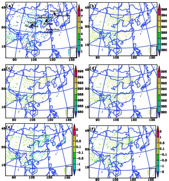
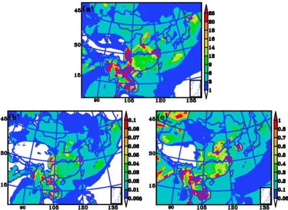
Figure 3. (a)Total number of observations in February 2010 in the model grid. Each symbol indicates the total number of all GOSAT XCO2 measurements in the corresponding model grid. Monthly mean values in February 2010 of(b)XpCO
2, column mixing ratio ofC
p
t;(c)XfCO2, column mixing ratio ofCft;(d)XaCO
2, column mixing ratio ofC
a t;(e)X
p CO2−X
f
CO2; and(f)X
p CO2−X
a
CO2. All column mixing ratios are column-averaged with real GOSAT XCO2averaging kernels at GOSAT XCO2locations. Each symbol indicates the monthly average value of all XCO2estimates in the model grid.C
a
t are the ensemble mean values of the assimilated CO2concentrations fields of a CFI-CMAQ OSSE,
in which the lag-window was 9 days andβwas 70. They are the same OSSE in Figs. 3–6.
the following). Then, the artificial GOSAT observationsyobst (or XpCO
2)were generated by substituting C
p
t into the ob-servation operator in Eq. (16). The retrieval information of GOSAT XCO2(y
priori,fpriori,handa
CO2)needed in Eq. (16) were gained from the v2.9 Atmospheric CO2Observations
from Space (ACOS) Level 2 standard data products, which only utilized the SWIR observations. Only data classified into the “Good” category were utilized in this study. Dur-ing the retrieval process, most of the soundDur-ings (such as data with a solar zenith angle greater than 85◦, or data not in clear sky conditions, or data collected over the ocean but not in glint, etc.) were not processed, so typically data products for
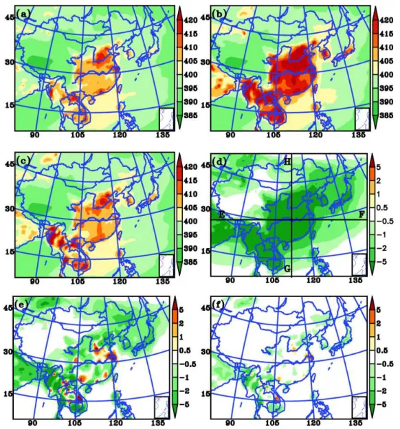
Figure 4.Monthly mean values of(a) Cpt, the artificial true simulations driven by the prior surface CO2fluxesFpt;(b) Cft, the background simulations driven by magnified surface CO2fluxesF∗t =(1.8+δ(x, y, z, t ))Fpt;(c) Cat, the ensemble mean values of the assimilated CO2 concentrations fields;(d) Cpt −Cft;(e) Cpt −Cat; and(f)100∗(Cpt −Cat).Cpt at model-level 1 in February 2010. Black lines EF and GH indicate the positions of the cross sections shown in Fig. 5.
Secondly, the prescribed surface CO2fluxes seriesF∗t were created by
F∗t =(1.8+δ(x, y, z, t ))Fpt, (25) whereδwas a random number. They were standard normal distribution time series at each grid in the integration pe-riod of our numerical experiment. Driven byF∗t, the RAMS-CMAQ model was integrated to obtain the CO2
simula-tions Cf(x, y, , z, t )(referred to asCft hereafter). Then, the column-averaged concentrations XfCO
2 were obtained using Eq. (16).
The performance of CFI-CMAQ was evaluated through a group of well-designed OSSEs, and the goal of each OSSE was to retrieve the true fluxes Fpt from given true
observa-tions XpCO
2 and “wrong” fluxes F ∗
t. In all the OSSEs, we assimilated artificial observations XpCO
2 about three times a day since GOSAT has about three orbits in the study model domain. If there were some observations, CFI-CMAQ paused to assimilate. Otherwise, it continued simulating. The default ensemble size N was 48, the measurement errors were 1.5 ppmv, the standard localization Schur radiuscwas 1280 km (20 grid spacing), and the covariance inflation fac-tor of concentrationsαwas 1.1. The referenced lag-window was 9 days and the covariance inflation factor of the prior scaling factorsβ was 70. Since the smoother window was very important for CO2 transportation and β was a newly
Figure 5.Monthly mean cross sections ofCpt−Cftalong line(a)EF and(b)GH, and monthly mean cross sections ofCpt−Cat along line(c)
EF and(d)GH (cross section lines shown in Fig. 4d) in February 2010.
primary focus of this paper was to describe the assimilation methodology, so all the numerical experiments started on 1 January 2010 and ended on 30 March 2010.
As for the initialization of CFI-CMAQ, only the ensemble of background concentration fieldsCi,f0needed to be initial-ized at the timet=0 because the values ofλai,t|t−1were up-dated using the persistence dynamical model. In practice, the mean concentration fields at t=0 are interpolated from the simulated CO2 fields of CarbonTracker 2011 (Peters et al.,
2007). The ensemble members of the background concen-tration fields were created by adding random vectors. The mean values of the random vectors were zero and the vari-ances were 2.5 percent of the mean concentration fields. The atmospheric transport model then integrated from timet=0 tot=1 driven byF∗t withCi,f0as initial conditions to pro-duce the CO2 concentration fields Cˆi,f1. Subsequently, the
first prior linear scaling factors,λpi,1|0, could be calculated by applyingCˆi,f1. Assuming thatλai,1|0=λpi,1|0,λai,1|0are gained, finally. For the first assimilation cycle, the lag-window was only one (that is, only λai,1|0needed to be optimized in the first assimilation cycle). It increased for the first dozens of as-similation cycles until it reached M+1 as CFI-CMAQ con-tinued to assimilate observations. Once the system was ini-tialized, all future scaling factors could be created using the persistence dynamical model, which associated the smooth-ing operator with the atmospheric transport model.
In order to illustrate the limitation using only the smooth-ing operator as the persistence dynamical model to gener-ate all future scaling factors, another OSSE (referred to as the reference experiment to distinguish it from the above-mentioned CFI-CMAQ OSSEs) was designed to optimize the surface CO2 fluxes at grid scale. The reference
exper-iment was under the same assimilation framework as CFI-CMAQ except that all λpi,t|t−1 were set to 1 (Peters et al., 2007). Beside that, the initialization procedure of the refer-ence experiment was different from that of the CFI-CMAQ. In practice, both the ensemble of background concentration fields att=0,Cfi,0, and the ensemble members of the scaling factors att=1,λai,1|0, needed to be initialized because they could not be generated in other ways (Peters et al., 2005). The initial concentration fieldsCi,f0 were created using the same method as that used to generateCfi,0for the CFI-CMAQ OSSEs. The ensemble members of the scaling factorsλai,1|0
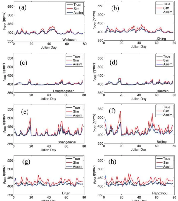
infla-Figure 6.Daily mean time series of CO2concentrations at national background stations in China and their nearest large cities from 1 January to 20 March 2010 extracted from the artificial true simulationsCpt (black), background simulationsCft(red), and the ensemble mean values of the assimilated CO2concentrations fieldsCat (blue). All time series were interpolated to the observation locations by the spatial bilinear interpolator method. The sites used are(a)Waliguan (36.28◦N, 100.91◦E),(b)Xining (36.56◦N, 101.74◦E),(c)Longfengshan (44.73◦N, 127.6◦E),(d)Haerbin (45.75◦N, 126.63◦E),(e)Shangdianzi (40.65◦N, 117.12◦E),(f)Beijing (39.92◦N, 116.46◦E),(g)Linan (30.3◦N, 119.73◦E), and(h)Hangzhou (30.3◦N, 120.2◦E).
tion factor of concentrationsαwas 1.1, and the lag-window was 9 days.
3.2 Experimental results
Essentially, the assimilation part of CFI-CMAQ includes two subsections: one for the CO2concentration assimilation with
EnKF, which can provide convincing CO2 initial analysis
fields for the next assimilation cycle; and the other for the CO2 flux optimization with EnKS, which can provide
bet-ter estimation of the scaling factors for the next time through the persistence dynamical model, except for optimized CO2
re-Figure 7.Monthly mean values in February 2010 of(a) Fpt, the prior true surface CO2fluxes;(b) F∗t, the prescribed CO2surface fluxes, F∗t =(1.8+δ(x, y, z, t ))Fpt;(c) Fat, the ensemble mean values of the assimilated surface CO2fluxes;(d) Fpt−F∗t; and(e) F
p
t −Fat (units: µmole m−2s−1).Fat are the assimilated results of a CFI-CMAQ OSSE, in which the lag-window was 9 days andβwas 70. They are the same in Figs. 7–10.
sults of a CFI-CMAQ OSSE, in which the lag-window was 9 days andβwas 70. The sensitivities ofβand the lag-window will then be discussed in the following two paragraphs. Fi-nally, the assimilation results of the reference experiment in whichλpi,t|t−1were set to 1 will be briefly described at the end of this subsection.
We begin by describing the impacts of assimilating artifi-cial observations XpCO
2 on CO2simulations by CFI-CMAQ. As shown in Fig. 4a, b and d, the monthly mean values of the background CO2concentrationsCft produced by the magni-fied surface CO2fluxesF∗t were much larger than those of the artificial true CO2concentrationsCpt produced by the prior surface CO2 fluxes Fpt near the surface in February 2010. In the east and south of China especially, the magnitude of
the difference betweenCpt andCft was at least 6 ppmv. Also, as expected, the monthly mean XfCO
2 was much larger than the monthly mean artificial observations XpCO
2, and the mag-nitude of the difference between XpCO
2 and X
f
CO2 reached 2 ppmv in the east and south of China (see Fig. 3b, c, e). However, the impact of magnifying surface CO2 fluxes on
the CO2concentrations was primarily below the model-level
10 (approximately 6 km), and especially below model-level 7 (approximately 1.6 km). Above model-level 10, the differ-ences betweenCpt andCft fell to zero (see Fig. 5a, b). After assimilating XpCO
2, the analysis CO2concentrationsC
Figure 8. Monthly mean RMSEs ofFat in February 2010 (units: µmole m−2s−1).
the relative error (Cpt –Cat)/C p
t ranged from−1 to 1 % in al-most the entire model domain at model-level 1. The monthly mean differences betweenCpt andCat were negligible above model-level 2 (see Fig. 5c, d). The monthly mean XaCO
2 was also closer to XpCO
2 and the difference between X
p CO2 and XaCO
2 ranged from −0.5 to 0.5 ppmv. In order to evaluate the general impact of assimilating XpCO
2 in the surface layer, time series of the daily mean CO2 concentration extracted
from the background simulations and the assimilations were compared with the artificial true simulations at four national background stations in China and their nearest large cities. As shown in Fig. 3a, Waliguan is 150 km away from Xin-ing, Longfengshan is 180 km away from Haerbin, Shangdi-anzi is 150 km away from Beijing, and Linan is 50 km away from Hangzhou. The assimilated results are shown in Fig. 6. The background time series were much larger than the ar-tificial true time series, especially at Shangdianzi, Beijing, Linan and Hangzhou, which are strongly influenced by local anthropogenic CO2emissions. After assimilating XpCO2, the assimilated time series were very close to the true time se-ries with negligible bias, as expected, at Waliguan, Xining, Shangdianzi, Beijing, Linan and Hangzhou, especially after the first 10 days, which can be considered the spin-up period. Meanwhile, the improvements at Longfengshan and Haerbin were limited due to the absence of observation data at those locations (see Fig. 3a). Nevertheless, in general, the substan-tial benefits to the CO2 concentrations in the surface layer
of assimilating GOSAT XCO2 with EnKF are clear. All the results illustrated that CFI-CMAQ can provide a convincing CO2initial analysis fields for CO2flux inversion.
The impacts of assimilating XpCO
2 on surface CO2fluxes were also highly impressive by CFI-CMAQ. On the whole, the prescribed CO2surface fluxesF∗t were much larger than the true surface CO2fluxesFpt in February 2010, especially in the east and south of China. The monthly mean differ-ence between F∗t andFpt reached 5 µmole m−2s−1 in Jing– Jin–Ji, the Yangtze River delta, and the Pearl River Delta Ur-ban Circle because of the strong local anthropogenic CO2
emissions (see Fig. 7a, b, d). After assimilating XpCO 2, the ensemble mean of the assimilated surface CO2fluxesFat de-creased sharply. Thus, the monthly mean values ofFat were much smaller thanF∗t in most of the model domain in Febru-ary 2010. The pattern of the difference betweenFat andF∗t was similar to that of the difference betweenFpt andF∗t (see Fig. 7d). The ensemble mean of the assimilated surface CO2
fluxesFat were also compared to the artificial true fluxesFpt, revealing thatFat was equivalent toFpt in most of the model domain. The monthly mean difference between Fat and Fpt ranged from−0.1 to 0.1 µmole m−2s−1 only (see Fig. 7e). In addition, the root-mean-square errors (RMSEs) of the as-similated flux members were analysed. As shown in Fig. 8, the monthly mean RMSE was less than 0.5 µmole m−2s−1 in most of the model domain, except in areas near to large cities such as Beijing, Shanghai and Guangzhou, indicating that the assimilated CO2fluxes were reliable.
In order to evaluate the ability of CFI-CMAQ to optimize the surface CO2 fluxes comprehensively, the ratios of the
monthly meanF∗t to the monthly meanFptwere analysed. In actual implementation, we only analysed the ratios where the absolute values of the monthly meanFpt were larger than 0.1, to avoid random noise. As shown in Fig. 9a, the ratios of the monthly meanF∗t to the monthly meanFpt are about 1.8 in most of China, except in the Qinghai–Tibet Plateau, where the absolute values of the monthly meanFpt in February were very small and were not analysed. In addition, the ratios of the monthly meanFat to the monthly meanFpt are shown in Fig. 9b. This figure demonstrates that the impact of the as-similation of XpCO
2 by CFI-CMAQ on CO2fluxes was great in the east and south of China in general, but the influence was negligible in Northeast China due to the lack of observa-tion data.
Time series of daily mean surface CO2 fluxes extracted
from F∗t andFat were also compared with that from Fpt at four national background stations in China and their near-est large cities, similar to the CO2 concentration
assimi-lation. The results are shown in Fig. 10. The background time series were much larger than the artificial true time se-ries, especially at Haerbin, Shangdianzi, Beijing, Linan and Hangzhou, which are strongly influenced by local anthro-pogenic CO2emissions. After assimilating X
p
CO2, the assim-ilated time series were near to the true time series with ac-ceptable bias, as expected, at Waliguan, Xining, Shangdianzi, Linan and Hangzhou after the 10-day spin-up period. How-ever, the improvements at Longfengshan and Haerbin were negligible because of a lack of observations at these loca-tions. Also, this inversion system failed to show improve-ments in Beijing. One of the possible reasons was that the values of the ensemble spread ofλai,t|t−1in the Beijing area are too large (see Fig. 11c). Beijing is located in the Jing– Jin–Ji Urban Circle, which had strong local anthropogenic CO2emissions during January–March. So the values of the
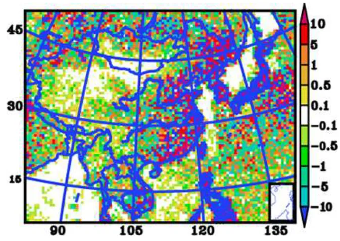
Figure 9. (a)Ratios of monthly meanF∗tto monthly meanFpt; and(b)ratios of monthly meanFat to monthly meanFpt in February 2010. The white part indicates the ratios where the absolute values of monthly meanFpt are larger than 0.1, not analysed in this study. The black square labelled I indicates the domain where surface CO2fluxes were used for the results presented in Figs. 12 and 13.
Figure 10.Daily mean time series of CO2fluxes at national background stations in China and their nearest large cities from 1 January to
Figure 11. (a)Ensemble spread ofCfi,t after inflating;(b)ensemble spread ofλp
i,t|t−1before inflating;(c)ensemble spread ofλ a i,t|t−1at
model-level 1 at 00:00 UT on 1 March 2010, whenβ=70.
Figure 12.Time series of daily mean CO2fluxes averaged in
do-main I (shown in Fig. 9a) from 1 January to 20 March 2010 with the inflation factor of scaling factorsβ=50,60,70,75 and 80. The black dashed line is the time series averaged fromF∗t and the black solid line is the time series averaged fromFpt.
could be much larger than those in other areas, which had weak local anthropogenic CO2emissions (see Fig. 11a). As
a result, the values of the ensemble spread ofλpi,t|t−1before inflating in the Beijing area are much larger than those in other areas with small local anthropogenic CO2 emissions
(see Fig. 11b). After inflating, the ensemble spread ofλpi,t|t−1
in the Beijing area could be too large, compared to those in other areas with small local anthropogenic CO2 emissions
(see Fig. 11c), which led to the failure to reproduce the true fluxes in the Beijing area. Later, CFI-CMAQ will be im-proved by optimizing the covariance inflation method.
Since the impact of assimilation XpCO
2 by CFI-CMAQ on CO2 fluxes was in general greater in the east and south of
China than other model areas (see Figs. 7, 9), the time series of the daily mean CO2fluxes in that area averaged fromFat was compared with those fromF∗t andFpt(see Fig. 12). This figure indicates that CFI-CMAQ could in general reproduce the true fluxes with acceptable bias.
As stated in the above section,β was a newly introduced parameter. The prior scaling factors should have been in-flated indirectly through the inin-flated CO2concentration
fore-cast. However, the values of the ensemble spread ofλpi,t|t−1
Figure 13.Time series of daily mean CO2fluxes averaged in
do-main I (shown in Fig. 9a) from 1 January to 20 March 2010 with different smoother windows (3, 6, 9 and 12 days). The black dashed line is the time series averaged fromF∗t and the black solid line is the time series averaged fromFpt.
smaller than 50 (e.g.β=10), the impact of assimilation was small due to the small ensemble spread; or if β was much larger than 80 (e.g.β=100), the assimilated CO2fluxes
de-viated markedly from the “true” CO2fluxes. In other words,
the performance of CFI-CMAQ greatly relies on the choice ofβ.
From the perspective of the lag-window, the differences among the four assimilation sensitivity experiments with lag-windows of 3, 6, 9 and 12 days were very small (see Fig. 13). Although Peters et al. (2007) indicated that the lag-window should be more than five weeks, it seemed that the smoother window had a slight influence on the assimilated results for CFI-CMAQ. It was clear that the assimilated results with a larger lag-window were better than those with a smaller lag-window; however, CFI-CMAQ performed very well even with a short lag-window (e.g. 3 days).
At the end of this subsection, the assimilation results of the reference experiment in whichλpi,t|t−1were set to 1 will be addressed briefly. The impact of assimilation XpCO
2 on CO2 fluxes was disordered. The monthly mean values of the dif-ference between the prior true surface CO2 fluxes and the
ensemble mean values of the assimilated surface CO2fluxes
were irregular noise (see Fig. 14). The main reason is that all the elements of the scaling factors to be optimized in the smoother window are only random numbers. As stated in the above section, onlyλai,1|0needed to be optimized in the first assimilation cycle. However,λai,1|0were rand fields (in other words, all the elements of λai,1|0 are random numbers) be-cause they could not be generated in other ways in the first instance. Therefore their spatial correlations were too small. The correlations between the scaling factors and the observa-tions were also too small. It was therefore impossible to sys-tematically change the values of λai,1|0 in large areas where the observations located after assimilating observations at t=1. Hence, the signal-to-noise problem arose. So, the ele-ments ofλai,1|1are also only random numbers. Thoughλai,2|1
Figure 14.Monthly mean values of the difference between the prior true surface CO2fluxes and the ensemble mean values of the
assim-ilated surface CO2fluxes (units: µmole m−2s−1)of the reference
experiment in whichλpi,t|t−1were set to 1.
could be generated automatically by the smoothing opera-tor when allλpi,2|1 were set to 1, the elements ofλai,2|1 are also random numbers because the smoothing operator is only a linear operator. Similarly, it was impossible to systemati-cally change the values ofλai,1|1andλai,2|1in large areas after assimilating observations att=2. As this inversion system continued assimilating observations, all future scaling fac-tors could be created by the smoothing operator and then updated. But this inversion system could not ingest the ob-servations effectively because all the elements of the scaling factors were always random numbers. Though the 9-day lag-window in the reference experiment is too short compared to the 5 week lag-window recommended by Peters et al. (2007), this reference experiment could illustrate the limitation by only using the smoothing operator as the persistence dynam-ical model. If the lag-window was around 5 weeks, we could achieve better results because there were more observations in every assimilation cycle. However, the results could not be better than those obtained by CFI-CMAQ because most grids have no observations (see Fig. 3a) and the signal-to-noise problem still remained.
4 Summary and conclusions
A regional surface CO2flux inversion system, CFI-CMAQ,
has been developed to optimize CO2fluxes at grid scales. It
operates under a joint data assimilation framework by apply-ing EnKF to constrain the CO2concentrations and applying
EnKS to optimize the surface CO2flux, which is similar to
con-stitute the persistence dynamical model to forecast the sur-face CO2flux scaling factors for the purpose of resolving the
“signal-to-noise” problem, as well as transporting the useful observed information onto the next assimilation cycle. In this application, the scaling factors to be optimized in the flux inversion system can be forecast at the grid scale without random noise. The OSSEs showed that the performance of CFI-CMAQ is effective and promising. In general, it could reproduce the true fluxes at the grid scale with acceptable bias.
This study represents the first step in developing a regional surface CO2 flux inversion system to optimize CO2 fluxes
over East Asia, particularly over China. In future, we in-tend to further develop the covariance localization techniques and inflation techniques to improve the performance of CFI-CMAQ. Furthermore, the uncertainty of the boundary con-ditions should be considered to improve the effectiveness of regional CO2flux optimization.
Acknowledgements. This work was supported by the National
Natural Science Foundation of China (grant no. 41130528), the Strategic Priority Research Program – Climate Change: Carbon Budget and Relevant Issues (XDA05040404), and the National High Technology Research and Development Program of China (2013AA122002). CarbonTracker results used to generate the initial condition were provided by NOAA ESRL, Boulder, Col-orado, USA from the website http://carbontracker.noaa.gov. The numerical calculations in this paper were done on the IBM Blade cluster system in the High Performance Computing Center (HPCC) of Nanjing University.
Edited by: X. Liu
References
Ahmadov, R., Gerbig, C., Kretschmer, R., Körner, S., Rödenbeck, C., Bousquet, P., and Ramonet, M.: Comparing high resolution WRF-VPRM simulations and two global CO2 transport
mod-els with coastal tower measurements of CO2, Biogeosciences, 6, 807–817, doi:10.5194/bg-6-807-2009, 2009.
Andres, R. J., Boden, T. A., Bréon, F.-M., Ciais, P., Davis, S., Erick-son, D., Gregg, J. S., JacobErick-son, A., Marland, G., Miller, J., Oda, T., Olivier, J. G. J., Raupach, M. R., Rayner, P., and Treanton, K.: A synthesis of carbon dioxide emissions from fossil-fuel com-bustion, Biogeosciences, 9, 1845–1871, doi:10.5194/bg-9-1845-2012, 2012.
Baker, D. F., Doney, S. C., and Schimel, D. S.: Variational data as-similation for atmospheric CO2, Tellus B, 58, 359–365, 2006. Boden, T. A., Marland, G., and Andres, R. J.: Global,
re-gional, and national fossil-fuel CO2 emissions, Carbon
Diox-ide Information Analysis Center, Oak Ridge National Labo-ratory, US Department of Energy, Oak Ridge, Tenn., USA, doi:10.3334/CDIAC/00001_V2011, 2011.
Chevallier, F.: Impact of correlated observation errors on inverted CO2 surface fluxes from OCO measurements, Geophys. Res. Lett., 34, L24804, doi:10.1029/2007GL030463, 2007.
Chevallier, F. M. F., Peylin, P., Bousquet, S. S. P., Bréon, F.-M., Chédin, A., and Ciais, P.: Inferring CO2sources and sinks from
satellite observations: Method and application to TOVS data, J. Geophys. Res., 110, D24309, doi:10.1029/2005JD006390, 2005. Chevallier, F., Bréon, F.-M., and Rayner, P. J.: Contribution of the Orbiting Carbon Observatory to the estimation of CO2 sources and sinks: Theoretical study in a variational
data assimilation framework, J. Geophys. Res., 112, D09307, doi:10.1029/2006JD007375, 2007.
Connor, B. J., Bösch, H., Toon, G., Sen, B., Miller, C., and Crisp, D.: Orbiting Carbon Observatory: Inverse method and prospective error analysis, J. Geophys. Res., 113, D05305, doi:10.1029/2006JD008336, 2008.
Crisp, D., Bösch, H., Brown, L., Castano, R., Christi, M., Con-nor, B., Frankenberg, C., McDuffie, J., Miller, C. E., Natraj, V., O’Dell, C., O’Brien, D., Polonsky, I., Oyafuso, F., Thompson, D., Toon, G., and Spurr, R.: OCO (Orbiting Carbon Observatory)-2 Level Observatory)-2 Full Physics Retrieval Algorithm Theoretical Ba-sis, Tech. Rep. OCO D-65488, NASA Jet Propulsion Labora-tory, California Institute of Technology, Pasadena, CA, version 1.0 Rev 4, http://disc.sci.gsfc.nasa.gov/acdisc/documentation/ OCO-2_L2_FP_ATBD_v1_rev4_Nov10.pdf, (last access: 4 Au-gust 2014), 2010.
Crisp, D., Fisher, B. M., O’Dell, C., Frankenberg, C., Basilio, R., Bösch, H., Brown, L. R., Castano, R., Connor, B., Deutscher, N. M., Eldering, A., Griffith, D., Gunson, M., Kuze, A., Man-drake, L., McDuffie, J., Messerschmidt, J., Miller, C. E., Morino, I., Natraj, V., Notholt, J., O’Brien, D. M., Oyafuso, F., Polonsky, I., Robinson, J., Salawitch, R., Sherlock, V., Smyth, M., Suto, H., Taylor, T. E., Thompson, D. R., Wennberg, P. O., Wunch, D., and Yung, Y. L.: The ACOS CO2retrieval algorithm – Part II:
Global XCO2data characterization, Atmos. Meas. Tech., 5, 687– 707, doi:10.5194/amt-5-687-2012, 2012.
Deng, F., Chen, J. M., Ishizawa, M., YUEN, C. W. A. I., Mo, G., Higuchi, K., Chan, D., and Maksyutov, S.: Global monthly CO2 flux inversion with a focus over North America, Tellus B, 59, 179–190, 2007.
Engelen, R. J., Serrar, S., and Chevallier, F.: Four-dimensional data assimilation of atmospheric CO2 using AIRS observations, J.
Geophys. Res., 114, D03303, doi:10.1029/2008JD010739, 2009. Feng, L., Palmer, P. I., Bösch, H., and Dance, S.: Estimating surface CO2fluxes from space-borne CO2dry air mole fraction obser-vations using an ensemble Kalman Filter, Atmos. Chem. Phys., 9, 2619–2633, doi:10.5194/acp-9-2619-2009, 2009.
Feng, L., Palmer, P. I., Yang, Y., Yantosca, R. M., Kawa, S. R., Paris, J.-D., Matsueda, H., and Machida, T.: Evaluating a 3-D transport model of atmospheric CO2 using ground-based,
air-craft, and space-borne data, Atmos. Chem. Phys., 11, 2789– 2803, doi:10.5194/acp-11-2789-2011, 2011.
Gurney, K. R., Law, R. L., Denning, A. S., Rayner, P. J., Baker, D., Bousquet, P., Bruhwiler, L., Chen, Y. H, Ciais, P., Fan, S., Fung, I. Y., Gloor, M., Heimann, M., Higuchi, K., John, J, Maki, T., Maksyutov, S., Masarie, K., Peylin, P., Prather, M., Pak, B. C., Randerson, J., Sarmiento, J., Taguchi, S., Takahashi, T., Yuen, C. W.: Towards robust regional estimates of CO2sources and
sinks using atmospheric transport models, Nature, 415, 626–630, 2002.
fos-sil fuel combustion CO2emission fluxes for the United States, Environ. Sci. Technol., 43, 5535–5541. doi:10.1021/es900806c, 2009.
Houtekamer, P. L. and Mitchell, H. L.: A sequential ensemble Kalman filter for atmospheric data assimilation, Mon. Weather Rev., 129, 123–137, 2001.
Huang, Z. K., Peng, Z., Liu, H. N., Zhang, M. G.: Development of CMAQ for East Asia CO2data assimilation under an EnKF
framework: a first result, Chinese Sci. Bull., 59, 3200–3208, doi:10.1007/s11434-014-0348-9, 2014.
Jiang, F., Wang, H. W., Chen, J. M., Zhou, L. X., Ju, W. M., Ding, A. J., Liu, L. X., and Peters, W.: Nested atmospheric inversion for the terrestrial carbon sources and sinks in China, Biogeosciences, 10, 5311–5324, doi:10.5194/bg-10-5311-2013, 2013.
Kang, J.-S., Kalnay, E., Liu, J., Fung, I., Miyoshi, T., and Ide, K.: “Variable localization” in an ensemble Kalman filter: applica-tion to the carbon cycle data assimilaapplica-tion, J. Geophys. Res., 116, D09110, doi:10.1029/2010JD014673, 2011.
Kang, J.-S., Kalnay, E., Miyoshi, T., Liu, J., and Fung, I.: Estimation of surface carbon fluxes with an advanced data assimilation methodology, J. Geophys. Res., 117, D24101, doi:10.1029/2012JD018259, 2012.
Kou, X., Zhang, M., Peng, Z.: Numerical Simulation of CO2
Con-centrations in East Asia with RAMS-CMAQ, Atmos, Oceanic Sci. Lett., 6, 179–184, 2013.
Kretschmer, R., Gerbig, C., Karstens, U., and Koch, F.-T.: Error characterization of CO2vertical mixing in the atmospheric
trans-port model WRF-VPRM, Atmos. Chem. Phys., 12, 2441–2458, doi:10.5194/acp-12-2441-2012, 2012.
Liu, J., Fung, I., Kalnay, E., Kang, J.: CO2transport uncertainties
from the uncertainties in meteorological fields, Geophys. Res. Lett., 38, L12808, doi:10.1029/2011GL047213, 2011.
Liu, J., Fung, I., Kalnay, E., Kang, J.-S., Olsen, E. T., and Chen, L.: Simultaneous assimilation of AIRS Xco2 and
me-teorological observations in a carbon climate model with an ensemble Kalman filter, J. Geophys. Res., 117, D05309, doi:10.1029/2011JD016642, 2012.
Liu Z., Bambha, R. P., Pinto, J. P.: Toward verifying fossil fuel CO2 emissions with the Community Multi-scale Air
Qual-ity (CMAQ) model: motivation, model description and ini-tial simulation. J. Air Waste Manage. Assoc., 64, 419–435, doi:10.1080/10962247.2013.816642, 2013.
Marland, G.: Uncertainties in accounting for CO2 from fossil
fuels, J. of Indust. Ecol., 12, 136–139, doi:10.1111/j.1530-9290.2008.00014.x, 2008.
Miyazaki K.: Performance of a local ensemble transform Kalman filter for the analysis of atmospheric circulation and distribu-tion of long-lived tracers under idealized condidistribu-tions, J. Geophys. Res., 114, D19304, doi:10.1029/2009JD011892, 2009.
National Research Council (NRC): Verifying greenhouse gas emis-sions: Methods to support international climate agreements, The National Academies Press, Washington, DC, available at: http: //www.nap.edu/download.php?record_id=12883 (last access: 27 January 2015), 2010.
O’Dell, C. W., Connor, B., Bösch, H., O’Brien, D., Frankenberg, C., Castano, R., Christi, M., Eldering, D., Fisher, B., Gunson, M., McDuffie, J., Miller, C. E., Natraj, V., Oyafuso, F., Polonsky, I., Smyth, M., Taylor, T., Toon, G. C., Wennberg, P. O., and Wunch, D.: The ACOS CO2retrieval algorithm – Part 1: Description and
validation against synthetic observations, Atmos. Meas. Tech., 5, 99–121, doi:10.5194/amt-5-99-2012, 2012.
Osterman, G., Martinez, E., Eldering, A., and Avis, C.: ACOS Level 2 Standard Product Data User’s Guide, v2.9, available at: http://oco.jpl.nasa.gov/files/ocov2/v2.9_DataUsersGuide_ RevD_20121026.pdf.pdf (last access: 27 January 2015), 2011. Peters, W., Miller, J. B., Whitaker, J., Denning, A. S., Hirsch, A.,
Krol, M. C., Zupanski, D., Bruhwiler, L., and Tans, P. P.: An en-semble data assimilation system to estimate CO2surface fluxes
from atmospheric trace gas observations, J. Geophys. Res., 110, D24304, doi:10.1029/2005JD006157, 2005.
Peters, W., Jacobson, A. R., Sweeney, C., Andrews, A. E., Conway, T. J., Masarie, K., Miller, J. B., Bruhwiler, L. M. P., Petron, G., Hirsch, A. I., Worthy, D. E. J., van der Werf, G. R.,Randerson, J. T., Wennberg, P. O., Krol, M. C., and Tans, P. P.: An atmospheric perspective on North American carbon dioxide exchange: Car-bonTracker, P. Natl. Acad. Sci. USA, 104, 18925–18930, 2007. Peters, W., KROL, M. C., Van Der WERF, G. R., Houwling, S.,
Jones, C. D., Hughes, J., Schaefer, K., Masarie, K. A., Jacob-son, A. R., Miller, J. B., Cho, C. H., Ramonet, M., Schmidt, M., Ciattaglia, L., Apadula, F., Heltai, D., Meinhardt, F., Di Sarra, A. G., Piachentina, S., Sferlazzo, D., Aalto, T., Hatakka, J., Ström, J., Haszpra, L., Meijer, H. A. J., Van Der Laan, S., Neubert, R. E. M., Jordan, A., Rodo, X., Morgui, J. –A., Vermeulen, A. T., Popa, E., Rozanski, M., Manning, A. C., Leuenberger, M., Uglietti, C., Dolman, A. J., Ciais, P., Heimann, M., Tans, P. P.: Seven years of recent Europenan net terrestrial carbon dioxide exchange con-strained by atmisppheric observations, Glob. Change Biol., 16, 1365–2486, 2009.
Peylin, P., Law, R. M., Gurney, K. R., Chevallier, F., Jacobson, A. R., Maki, T., Niwa, Y., Patra, P. K., Peters, W., Rayner, P. J., Rödenbeck, C., van der Laan-Luijkx, I. T., and Zhang, X.: Global atmospheric carbon budget: results from an ensemble of atmospheric CO2 inversions, Biogeosciences, 10, 6699–6720,
doi:10.5194/bg-10-6699-2013, 2013.
Pillai, D., Gerbig, C., Ahmadov, R., Rödenbeck, C., Kretschmer, R., Koch, T., Thompson, R., Neininger, B., and Lavrié, J. V.: High-resolution simulations of atmospheric CO2over complex
terrain – representing the Ochsenkopf mountain tall tower, At-mos. Chem. Phys., 11, 7445–7464, doi:10.5194/acp-11-7445-2011, 2011.
Prather, M., Zhu, X., Strahan, S.E., Steenrod, S., D., and Ro-driguez, J., M.: Quantifying errors in trace species trans-port modeling, P. Natl. Acad. Sci. USA, 105, 19617–19621. doi:10.1073/pnas.0806541106, 2008.
Tangborn, A., Strow, L. L., Imbiriba, B., Ott, L., and Pawson, S.: Evaluation of a new middle-lower tropospheric CO2 product
using data assimilation, Atmos. Chem. Phys., 13, 4487–4500, doi:10.5194/acp-13-4487-2013, 2013.
Tian, X., Xie, Z., and Sun, Q.: A POD-based ensemble four-dimensional variational assimilation method, Tellus A, 63, 805– 816, 2011.
Tian, X., Xie, Z., Liu, Y., Cai, Z., Fu, Y., Zhang, H., and Feng, L.: A joint data assimilation system (Tan-Tracker) to simultaneously estimate surface CO2 fluxes and 3-D atmospheric CO2
con-centrations from observations, Atmos. Chem. Phys., 14, 13281-13293, doi:10.5194/acp-14-13281-2014, 2014.
van Leeuwen, T. T.: Global fire emissions and the contribution of deforestation, savanna, forest, agricultural, and peat fires (1997– 2009), Atmos. Chem. Phys., 10, 11707–11735, doi:10.5194/acp-10-11707-2010, 2010.
Wang, B., Liu, J., Wang, S., Cheng, W., Liu, J., Liu, C., Xiao Q., and Kuo, Y.: An economical approach to four-dimensional variational data assimilation, Adv. Atmos. Sci., 27, 715–727, doi:10.1007/s00376-009-9122-3, 2010.
Zhang, H. F., B. Z. Chen, I. T. van der Laan-Luijkx, J. Chen, G. Xu, J. W. Yan, L. X. Zhou, Y. Fukuyama, P. P. Tans, and W. Peters, Net terrestrial CO2exchange over China during 2001–
2010 estimated with an ensemble data assimilation system for atmospheric CO2, J. Geophys. Res. Atmos., 119, 3500–3515,
doi:10.1002/2013JD021297, 2014a.
Zhang, H. F., Chen, B. Z., van der Laan-Luijk, I. T., Machida, T., Matsueda, H., Sawa, Y., Fukuyama, Y., Langenfelds, R., van der Schoot, M., Xu, G., Yan, J. W., Cheng, M. L., Zhou, L. X., Tans, P. P., and Peters, W.: Estimating Asian terrestrial carbon fluxes from CONTRAIL aircraft and surface CO2observations for the period 2006–2010, Atmos. Chem. Phys., 14, 5807–5824, doi:10.5194/acp-14-5807-2014, 2014b.
Zhang, M., Uno, I., Sugata, S., Wang, Z., Byun, D., Akimoto, H.: Numerical study of boundary layer ozone transport and photo-chemical production in East Asia in the wintertime, Geophys. Res. Lett., 29, 40-1–40-4, doi:10.1029/2001GL014368, 2002. Zhang, M., Uno, I., Carmichael, G. R., Akimoto, H., Wang, Z.,
Tang, Y., Woo, J., Streets, D. G., Sachse, G. W., Avery, M. A., Weber, R. J., Talbot, R. W.: Large-scale structure of trace gas and aerosol distributions over the western Pacific Ocean during the Transport and Chemical Evolution Over the Pa-cific (TRACE-P) experiment, J. Geophys. Res., 108, 8820, doi:10.1029/2002JD002946, 2003.