www.atmos-chem-phys.net/16/1729/2016/ doi:10.5194/acp-16-1729-2016
© Author(s) 2016. CC Attribution 3.0 License.
What do correlations tell us about anthropogenic–biogenic
interactions and SOA formation in the Sacramento plume
during CARES?
L. Kleinman1, C. Kuang1, A. Sedlacek1, G. Senum1, S. Springston1, J. Wang1, Q. Zhang2, J. Jayne3, J. Fast4, J. Hubbe4, J. Shilling4, and R. Zaveri4
1Brookhaven National Laboratory, Upton, NY, USA 2University of California at Davis, Davis, CA, USA 3Aerodyne Research Inc., Billerica, MA, USA
4Pacific Northwest National Laboratory, Richland, WA, USA
Correspondence to:L. Kleinman ([email protected])
Received: 7 July 2015 – Published in Atmos. Chem. Phys. Discuss.: 17 September 2015 Revised: 31 December 2015 – Accepted: 14 January 2016 – Published: 15 February 2016
Abstract. During the Carbonaceous Aerosols and Radia-tive Effects Study (CARES) the US Department of Energy (DOE) G-1 aircraft was used to sample aerosol and gas phase compounds in the Sacramento, CA, plume and surrounding region. We present data from 66 plume transects obtained during 13 flights in which southwesterly winds transported the plume towards the foothills of the Sierra Nevada. Plume transport occurred partly over land with high isoprene emis-sion rates. Our objective is to empirically determine whether organic aerosol (OA) can be attributed to anthropogenic or biogenic sources, and to determine whether there is a syn-ergistic effect whereby OA concentrations are enhanced by the simultaneous presence of high concentrations of carbon monoxide (CO) and either isoprene, MVK+MACR (sum of
methyl vinyl ketone and methacrolein), or methanol, which are taken as tracers of anthropogenic and biogenic emissions, respectively. Linear and bilinear correlations between OA, CO, and each of three biogenic tracers, “Bio”, for individ-ual plume transects indicate that most of the variance in OA over short timescales and distance scales can be explained by CO. For each transect and species a plume perturbation, (i.e., 1OA, defined as the difference between 90th and 10th per-centiles) was defined and regressions done amongst1values in order to probe day-to-day and location-dependent variabil-ity. Species that predicted the largest fraction of the variance in1OA were1O3and1CO. Background OA was highly
correlated with background methanol and poorly correlated
with other tracers. Because background OA was∼60 % of
peak OA in the urban plume, peak OA should be primarily biogenic and therefore non-fossil, even though the day-to-day and spatial variability of plume OA is best described by an anthropogenic tracer, CO. Transects were split into subsets according to the percentile rankings of 1CO and 1Bio, similar to an approach used by Setyan et al. (2012) and Shilling et al. (2013) to determine if anthropogenic–biogenic (A–B) interactions enhance OA production. As found earlier, 1OA in the data subset having high1CO and high1Bio was several-fold greater than in other subsets. Part of this differ-ence is consistent with a synergistic interaction between an-thropogenic and biogenic precursors and part to an indepen-dent linear dependence of1OA on precursors. The highest values of1O3, along with high temperatures, clear skies, and
poor ventilation, also occurred in the high1CO–high1Bio data set. A complicated mix of A–B interactions can result. After taking into account linear effects as predicted from low concentration data, an A–B enhancement of OA by a factor of 1.2 to 1.5 is estimated.
1 Introduction
(SOA) is derived from biogenic precursors but its forma-tion depends on interacforma-tions between urban anthropogenic emissions and a larger, geographically dispersed pool of bio-genic emissions, hereinafter referred to as A–B interactions (de Gouw et al., 2005; Weber et al., 2007; Goldstein et al., 2009; de Gouw and Jimenez, 2009; Carlton et al., 2010; Wor-ton et al., 2011; Xu et al., 2015). A–B interactions lie at the intersection of two problems. First is an explanation of unex-pectedly high concentrations of OA, which are most promi-nently noticed downwind of urban areas (e.g., Volkamer et al., 2006; Kleinman et al., 2008; Matsui et al., 2009). Sec-ond is the finding that a high fraction of OA consists of non-fossil carbon of biogenic origin, even downwind of urban ar-eas (Schichtel et al., 2008; Marley et al., 2009; Hodzic et al., 2010; Zotter et al., 2014).
Progress has been made on the problem of models predict-ing lower OA than observed. Older models (ca. pre 2005) are now recognized to contain a limited set of aerosol pre-cursors and aerosol formation mechanisms. Some part of the gap between observations and theory can be closed using up-dated models that contain new categories of anthropogenic compounds, chemical mechanisms, and physical interactions (e.g. Robinson et al., 2007; Hodzic et al., 2010). In order to agree with14C measurements, the gap has to be closed with a significant fraction of non-fossil carbon, which brings us back to the possibility of A–B interactions.
Evidence for, and mechanisms of, A–B interactions have been reviewed by Hoyle et al. (2011). Pertinent findings are that (1) the major source of volatile organic compounds (VOCs), globally and in many well-studied regions, such as the southeastern US and Canadian boreal forest, is bio-genic (e.g., Guenther et al., 1995; Goldstein et al., 2009; Slowik et al., 2010), (2) large biogenic emission rates and SOA yields are a possible cause for the high fraction of non-fossil carbon found in the summer in many locations (Schichtel et al., 2008; Hodzic et al., 2010), including those that are nominally urban (Weber et al., 2007; Marley et al., 2009), and (3) there are realistic mechanisms whereby bio-genic SOA yields depend on the presence of anthropobio-genic pollutants (Carlton et al., 2010). The latter include effects of anthropogenic pollutants on oxidant levels and consequently on biogenic VOC oxidation rates (Kanakidou et al., 2000), increased partitioning of biogenic VOC oxidation products to the aerosol phase because the aerosol volume, includ-ing associated water, available for partitioninclud-ing is increased by an anthropogenic component (Carlton et al., 2010; Carl-ton and Turpin, 2013), aqueous phase reactions (Ervens et al., 2011), and effects of sulfate on aerosol phase chemistry (Xu et al., 2015). Explanations of non-fossil carbon based on A–B interactions are constrained by the observation that the difference between modeled and observed OA concen-tration generally decreases as anthropogenic influence de-creases (Tunved et al., 2006; Chen et al., 2009; Hodzic et al., 2010; Slowik et al., 2010)
In multiple studies it has been found that OA, SOA, and/or WSOC (water soluble organic carbon; demonstrated to be a surrogate for SOA) are highly correlated with anthropogenic tracers. High correlations have been observed even at loca-tions where it is suspected that much if not most SOA is biogenic. In a study of the Atlanta region, aircraft flights over the urban core established that WSOC is proportional to carbon monoxide (CO), while surface observations of aerosol14C, also in the urban core, established that 70–80 % of WSOC was non-fossil and likely biogenic (Weber et al., 2007). While there was a high correlation between WSOC and CO in Atlanta, similar to that observed in the New York City metropolitan region (Sullivan et al., 2006), there was no clear linkage between WSOC and biogenic VOCs. At the Blodgett Forest Research Station, located 25 km downwind from the Carbonaceous Aerosols and Radiative Effects Study (CARES) sampling region, OA was observed to be correlated with CO (R2=0.79) but based on14C filter samples it was determined that the majority of aerosol carbon was non-fossil from biogenic sources (Worton et al., 2011). Although high correlations between OA and biogenic VOCs have been re-ported (e.g. Slowik et al., 2010), it is more typical that in regions with an urban influence, correlations are low and in general do not suggest a relation between SOA and biogenic precursors. In a set of global calculations having the objective of satisfying the dual constraints of matching observations of OA concentration and14C content, it was found that the best of many mechanisms considered was one in which the ge-ographic distribution of OA followed that of anthropogenic CO, but had a14C content appropriate to a biogenic precursor
(Spracklen et al., 2011).
An objective of the CARES field campaign, conducted in June 2010, was to determine whether and to what ex-tent the simultaneous occurrence of high concentrations of anthropogenic and biogenic compounds is associated with enhanced concentrations of OA. An overview of the field campaign is given by Zaveri et al. (2012) and a detailed description of the meteorology and emission source re-gions affecting the Sacramento plume provided by Fast et al. (2012). Effects of A–B interactions have been examined during the CARES campaign by Shilling et al. (2013) us-ing aircraft data from the G-1 and by Setyan et al. (2012) using data from the rural T1 surface site located 40 km northeast of Sacramento. Both studies considered the ratio (OA−background)/(CO−background) and found that this ratio increased by a factor of ∼3 when an anthropogeni-cally influenced air mass also contained high concentrations of biogenic VOCs. At a CO concentration, indicative of a significant anthropogenic impact, both studies find that OA concentrations are higher when the CO is accompanied by higher concentrations of biogenic VOCs.
lead to SOA. A comparison is made between calculations in which isoprene, methyl vinyl ketone and methacrolein (MVK+MACR), or methanol (CH3OH) were used as
trac-ers of biogenic emissions. Isoprene and MVK+MACR, in contrast to CO, have short atmospheric lifetimes; therefore, their presence only explicitly addresses biogenic inputs to an air mass over a few hours time span. CH3OH, has a primary
biogenic source and a lifetime of order 10 days (Schade and Goldstein, 2006; Wells et al., 2012) and therefore can provide information on biogenic inputs over a time span comparable to the lifetime of tropospheric aerosols.
In order to understand the roles of anthropogenic and biogenic tracers in describing SOA formation over spatial scales comparable to the Sacramento plume, correlation co-efficients between OA and explanatory variables have been determined for each plume transect. For the purpose of de-termining the sensitivity of OA to conditions that vary over the CARES campaign, we define for each plume transect and species a background concentration and plume pertur-bation, 1, and use these quantities in a regression analysis amongst transects. Transects are also split into subsets having the varying combination of low and high values for1CO and 1isoprene,1MVK+MACR or1CH3OH. We find that the
data subset with high concentrations of both anthropogenic and biogenic tracers has uniquely high values of1OA. This result is similar to the A–B enhancement found by Setyan et al. (2012) and Shilling et al. (2013). We consider whether the uniquely high values of1OA can be explained by an in-dependent linear dependence of1OA on anthropogenic and biogenic tracers, rather than a synergistic effect.
OA and its anthropogenic and biogenic precursors are expected to be mutually enhanced through a common de-pendence on meteorological conditions (e.g. ventilation, sunlight, and temperature) occurring in pollution episodes (Goldstein et al., 2009). Such conditions promote A–B inter-action and may also give rise to an altered, non-synergistic dependence of OA on precursors. Our analysis cannot distin-guish between causes of enhanced OA, leading us to equate the net effect of enhanced OA above that expected from a bi-linear model of low concentration data to an A–B interaction. We find a high correlation between1OA and1O3(Herndon
et al., 2008; Wood et al., 2010). Studies of the dependence of O3on meteorological factors and on anthropogenic and
bio-genic precursors have a long history and could yield insights on SOA production.
Although there is a high anthropogenic, high biogenic, subset that stands out as having high concentrations of1OA, most of the spatial variability of OA within a transect and 1OA amongst transect can be explained by CO or1CO, respectively. These observations suggest a primarily anthro-pogenic origin for OA produced in the Sacramento plume. In contrast, the variability of background OA is much bet-ter explained by background CH3OH, which suggests a
bio-genic origin. As background OA is more abundant than OA formed in the Sacramento plume, the plume OA, though
cor-relating best with CO, is expected to have a14C signature of non-fossil, biogenic carbon. The plume composition would then resemble that observed in Atlanta (Weber et al., 2007) and that observed in the afternoon outflow from Los Angeles (Zotter et al., 2014).
2 Experimental
Data for the CARES field campaign including the G-1 data used in this study can be accessed from DOE’s ARM (Atmo-spheric Radiation Measurement) Climate Research archive at http://www.archive.arm.gov. AMS (Aerosol Mass Spectrom-eter) and PTR-MS (Proton Transfer Reaction Mass Spec-trometer) data were recorded at the instrument cycle time of 13 and 4 s, respectively. Most other measurements were col-lected at 1 Hz. Data used in this study was interpolated or averaged to a 10 s time base. Units for aerosol concentration are µg m−3at 1013 mb and 23◦C. Trace gas abundances are expressed as mixing ratios in units of ppbv. When referring to aerosol and gas phase species collectively, the term con-centration is used.
2.1 Instruments
The primary chemical measurements used in the regres-sion analysis are (1) organic aerosol: designated hereinafter as OA, (2) CO: a surrogate for anthropogenic precursors of OA, (3) isoprene: MVK+MACR, and CH3OH,
sur-rogates for biogenic OA precursors, and (4) O3: a
prod-uct of OH-driven photochemistry. These species were mea-sured using an Aerodyne HR-Tof-AMS (High-Resolution Time-of-Flight Aerosol Mass Spectrometer), a VUV (vac-uum ultraviolet) resonance fluorescence detector built at BNL (Brookhaven National Laboratory), an Ionicon PTR-MS (Lindinger et al., 1998), and a TEI49 (Thermo Environ-mental Instruments) O3 detector, respectively. An overview
of instrumentation used in CARES is given in Zaveri et al. (2012).
Operational principals of the AMS are described by Cana-garatna et al. (2007) and references therein. Its use on the G-1 during CARES is described by Shilling et al. (2013). In brief, the AMS on the G-1 operated in V-mode, with the duty cycle devoted entirely to determining mass, rather than mass-resolved particle size. A pressure controlled inlet maintained constant volumetric flow at all flight altitudes. Aerosol en-tered the cabin through a two stage diffuser isokinetic inlet designed by Brechtel Manufacturing with a transmission ef-ficiency close to 100 % for particles smaller than∼3 µm. The
transmission efficiency of the AMS falls off above a vacuum aerodynamic diameter (dva)of 600 nm dropping to zero at
1.5 µm.
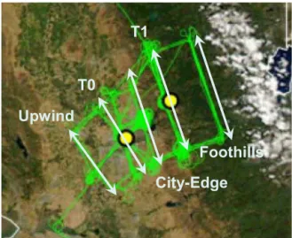
Upwind
T0
T1
City-Edge
Foothills
Figure 1.Map of sampling region, showing composite ground track for SW flights. Five transects more or less perpendicular to the boundary layer wind direction are indicated. Adapted from Zaveri et al. (2012).
CARES domain. Mixing ratios of monoterpenes were typi-cally close to the limit of detection and therefore could not be used to identify air masses influenced by biogenic emissions. 2.2 Flights
There were 22 research flights in CARES. Only boundary layer portions of flights with SW winds are considered here. Turbulent kinetic energy dissipation rate and the standard de-viation of vertical velocity were used to distinguish the con-vective boundary layer from the more quiescent free tropo-sphere. Flights selected make a relatively homogeneous set in terms of sampling locations. There were 14 such flights, one of which (623a) is not included in this analysis because of problems with the CO measurement. Flights are listed in Table 1. A composite ground track for the SW flights is given in Fig. 1. Proceeding in the direction of the wind, transects are identified as Upwind, T0, City-Edge, T1, and Foothills. Transects T0 and T1 passed over the similarly named ground sites. These five flight segments are more or less perpendicu-lar to the wind direction. Unfortunately there are no pairs of compounds that can be used for photochemical age. Organic aerosol O to C ratios reported by Shilling et al. (2013) are in a narrow range and thus not likely to provide information on aging.
Figure 1 shows a change in terrain color from brown to green at the T1 transect, indicating more vegetation to the east, which coincides with emission inventory estimates of higher isoprene emissions rates (Fast et al., 2012; Zaveri et al., 2012). The Foothills transect is at the western edge of a 20–25 km band of oak woodlands. Still further to the north-east there is a shift in vegetation, so that at the Blodgett Forest research station, 75 km from Sacramento, monoterpenes are the dominate source of SOA (Dreyfus et al., 2002).
Table 1.Flights used in study.
Flight Time (PST; hh:mm)
606a 09:35–12:42
606b 14:29–17:14
608a 07:56–11:12
608b 14:24–17:47
615a 07:57–11:01
615b 13:50–17:07
619a 14:26–17:29
623b 14:25–17:25
624a 07:56–11:11
624b 14:25–17:12
627a 09:24–12:47
628a 08:23–11:33
628b 14:21–16:42
2.3 Plumes
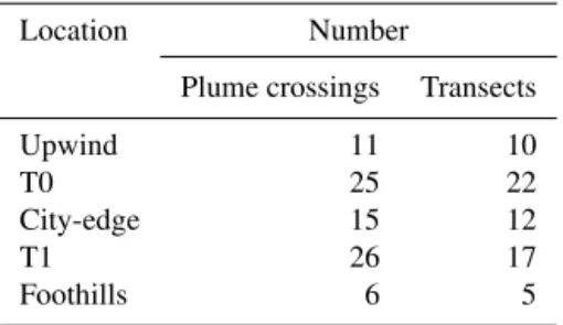
On many flights the Sacramento plume was crossed multiple times at the same location. If these crossings were consecu-tive, at the same altitude, and within the boundary layer, they were grouped together for the purpose of calculating concen-trations and for regression analysis. If plume crossings were separated in time or were at different altitudes they consti-tuted separate data entries. Henceforth, the termplume cross-ingwill refer to individual crossings whilst the term tran-sectcollapses consecutive crossings (that meet criteria given above) into a single entity. As listed in Table 2, there were a total of 83 plume crossings that made up 66 plume tran-sects. The number of 10 s data points in a single plume cross-ing is about 60. For each transect, frequency distributions for aerosol and trace gas concentration were determined. Back-ground concentrations are operationally defined by the 10th percentile. Perturbations above background were calculated as the difference between the 90th and 10th percentile of con-centration and are denoted by the symbol1.
3 Data analysis
In our analysis of the G-1 data set we consider variations in OA observed along a plume transect and a larger-scale variability that includes the effects of day-to-day changes in meteorology. Variations in OA are correlated with anthro-pogenic and biogenic explanatory variables, which are sur-rogates for the actual compounds that form SOA.
3.1 Tracers
emis-sion region, dilution causes concentrations of CO and OA to decrease. SOA is formed from photochemical processing of emitted pollutants while changes to CO aside from dilution are relatively minor (in the absence of downwind emission sources) causing the ratio OA/CO to increase with photo-chemical age (Sullivan et al., 2006; Weber et al., 2007; de Gouw et al., 2005, 2008; Kleinman et al., 2008). Formation of CO from oxidation of biogenic compounds is discussed by Shilling et al. (2013) and thought to be a small fraction of anthropogenic emissions for flights discussed herein. A com-parison of regression slopes measured on T0 transects with those measured on T1 transects shows considerable variabil-ity that averages out to a 54 % increase downwind, less than seen in other urban plumes. OA to CO ratios observed over T0 are several-fold greater than the lowest values observed in other urban centers where primary emissions are impor-tant (calculated from Zhang et al., 2005, 2007). This is in agreement with observations from T1 that show 90 % of OA is secondary (Setyan et al., 2012) and observations from the G-1 (Shilling et al., 2013) that show only minor changes in O to C ratios as a function of downwind distance. A factor contributing to a low range in processing is that the T0 site is 14 km downwind of the urban center and therefore OA ob-served on the T0 transect is already somewhat aged (Fast et al., 2012). Also, Sacramento urban emissions are spread out over a fetch nearly equal to the T0 to T1 distance, thereby blurring the distinction between urban and downwind chem-istry. An O to C signal for fresh emissions is further diluted by aged background aerosol from the San Francisco Bay area or from recirculation of the prior days plume into the residual layer over Sacramento.
Isoprene, first generation isoprene oxidation products MVK+MACR, and methanol were used as surrogate com-pounds to represent emitted biogenic VOCs responsible for SOA formation. As the atmospheric lifetime of isoprene with respect to OH oxidation is of an order of 1 h (at OH=3×10⁶molec cm−3), its presence in the atmosphere reflects local conditions rather than the longer time span over which SOA production is thought to occur. Because the re-action of MVK+MACR with OH is ∼3 to 4 times slower
than isoprene, atmospheric residence times are closer to the timescale for transport of the Sacramento plume within our sampling region. Transport times from the Sacramento ur-ban center to T1 have been calculated to be 2 to 8 h from WRF-Chem simulations (Fast et al., 2012). However, under high NOx conditions such as found in the photochemically
active regions of an anthropogenic plume, the formation of OA from isoprene emissions proceeds primarily from sec-ond and higher generation oxidation products rather than di-rectly from MVK+MACR (Ng et al., 2006; Carlton et al.,
2009). While there might not be a direct link between concur-rently measured isoprene or MVK+MACR and SOA, the
occurrence of high mixing ratios of isoprene and its oxida-tion products can indicate a potential for future SOA pro-duction or be a general indicator that meteorological
con-Table 2.Number of plume crossings and transects.
Location Number
Plume crossings Transects
Upwind 11 10
T0 25 22
City-edge 15 12
T1 26 17
Foothills 6 5
ditions such as temperature, sunlight, ventilation, and wind direction are favorable for the occurrence and accumulation of biogenic VOCs. Methanol, in contrast, addresses source attribution for biogenic aerosol in much the same way as CO is used as a tracer of anthropogenic SOA precursors. The at-mospheric lifetime of methanol is∼10 days and while not an SOA precursor, it is co-emitted with biogenic VOCs that are. Under conditions prevailing in the experimental area it is expected that the source of methanol is almost entirely bio-genic (Wells et al., 2012). Emission rates for CH3OH,
es-pecially the biogenic component from new leaf production, have a pronounced seasonal variability peaking in the spring and early summer (Schade and Goldstein, 2006; Wells et al., 2012), nearly coincident with the CARES field campaign. In other regions and at other times, a greater fraction of CH3OH
may derive from maritime sources, forest fires, or peroxy rad-ical combination reactions, which could compromise the util-ity of CH3OH as a tracer of biogenic aerosol precursors.
3.2 Regression analysis
A series of single variable and multi-variable regressions were performed using time series measurements for each of 66 transects. M1 to M5 designate the models used. Stan-dardized variables, indicated with a subscript S, have zero mean and unit standard deviation. The term “Bio” desig-nates a tracer of biogenic emission, which in this study is isoprene, MVK+MACR, or CH3OH. Models M1–M4 are
based on CO and Bio as explanatory variables. M4 uses a bilinear combination of CO and Bio and M3 measures multi-collinearity, the extent to which the two explanatory vari-ables, CO and Bio, are correlated. M5 is a linear relation between OA and O3.
The same models were used to compare backgrounds and concentration perturbations (e.g.1OA,1CO) amongst tran-sects. M1 to M5 are defined by
M1 OA=a1+B1CO
M2-Bio OA=a2+B2 BIOBio
M3-Bio CO=a3+B3 BIOBio
Table 3.Backgrounds averaged over transects at five locations.
Transect Background∗
MVK
OA CO Isoprene +MACR CH3OH O3
Upwind 3.9 127 0.29 0.18 4.7 35
T0 4.1 132 0.30 0.13 4.6 41
City-edge 4.8 133 0.26 0.11 4.4 53
T1 5.3 134 1.1 0.97 5.5 50
Foothills 4.2 133 1.9 1.5 5.1 57
∗Background is the lowest 10th percentile. Units are ppbv, except for organic aerosol
(OA), which is µg m−3.
M4S-Bio OAS=β4 COCOS+β4 BIOBioS
M5 OA=a5+B5O3,
where the a are intercepts and theB andβ are regression slopes. In order to improve legibility MVK+MACR will be shortened to MVK when used as a subscript. Quadratic mod-els with terms such as COStimes BioSwere also considered,
but did not yield insights or appreciable increases in perfor-mance.
For the standardized model, M4S, a comparison ofβ4 CO
withβ4 BIOgives the relative effect on OASof changing COS
and BioS by the same multiple of their respective standard
deviations. Standardization does not affect the value ofR2 nor does it change the signs of the coefficients of the explana-tory variables. Standardized coefficients can be expressed in terms of bivariate Pearson correlation coefficients as
β4 CO=(rOA CO−rOA BIO×rCO BIO)/(1−R2CO BIO), (1a)
β4 BIO=(rOA BIO−rOA CO×rCO BIO)/(1−R2CO BIO), (1b)
where, e.g.,rCO BIOis the correlation coefficient between CO
and Bio from M3. β4 CO and β4 BIO reduce to rOA CO and
rOA BIO, respectively, in the case that CO and Bio are
uncor-related.
In a three variable system spurious correlations arise be-cause two variables that are correlated with a third are neces-sarily correlated with each other (Panofsky and Brier, 1968). For example, in the system OA, CO, Bio there is a spuri-ous correlation between OA and CO due to both variables being correlated with Bio, given byrOA BIO×rCO BIO.
Like-wise, there is a spurious correlation between OA and Bio due to both variables being correlated with CO, given by rOA CO×rCO BIO. Numerators of Eq. (1a) and (1b) are
there-fore bivariate correlations of OA with CO and Bio, respec-tively, in excess of the corresponding spurious value. Be-cause CO and Bio can be highly correlated, both spurious correlations, can be large. For some transects, the linear mod-els M1 and M2 predict a strong correlation between vari-ables, while theβs in model M4Sare of opposite sign. Thus,
in some cases, the linear models can indicate that an
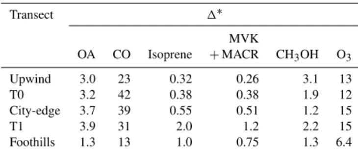
explana-Table 4.Plume perturbations,1s, averaged over transects at five locations.
Transect 1∗
MVK
OA CO Isoprene +MACR CH3OH O3
Upwind 3.0 23 0.32 0.26 3.1 13
T0 3.2 42 0.38 0.38 1.9 12
City-edge 3.7 39 0.55 0.51 1.2 15
T1 3.9 31 2.0 1.2 2.2 15
Foothills 1.3 13 1.0 0.75 1.3 6.4
∗
1is the 90th percentile–10th percentile. Units are ppbv, except for organic aerosol (OA), which is µg m−3.
tory variable promotes OA, while in the context of M4 or M4S, the opposite is true.
A two variable model (e.g. M4) is judged to be an im-provement over a single variable model (M1 or M2) accord-ing to whether the added variable produces a statistically sig-nificant increase inR2. Even if the added variable is random, R2will increase as long as the added variable is not a linear function of the explanatory variables already in use. The re-lation between linear and bilinear values ofR2can be found in Panofsky and Brier (1986, p. 112) and other statistics text books. Statistical significance is discussed in the Supplement where it is pointed out that because plumes are correlated structures with fewer degrees of freedom than data points, the usual ways of determining statistical significance, such as t or f tests, do not apply (Thiébaux and Zwiers, 1984; Trenberth, 1984).
4 Results
Tables 3 and 4 summarize chemical measurements from the G-1, providing backgrounds and plume perturbations for OA, CO, isoprene, MVK+MACR, CH3OH, and O3 averaged
over transects according to location. Background concentra-tions of the long-lived constituents, OA, CO, and CH3OH
are to the first order about the same on all five legs. The short-lived species, isoprene and MVK+MACR, increase by approximately an order of magnitude from east to west, following changes in emissions. Ozone is an intermediate case. Calling the 10th percentile of concentration “back-ground” comes closest to matching the traditional definition for species with long atmospheric residence time. Even so, backgrounds for OA, CO, and CH3OH have significant
vari-ability, which we will take advantage of for source attribution of OA.
4.1 Correlations for the spatial variability within individual transects
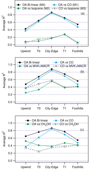
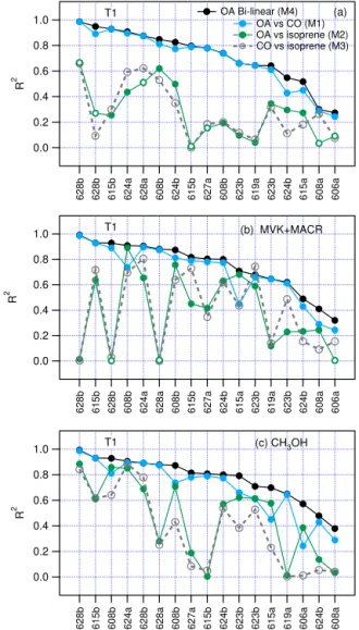
Figure 2 shows values ofR2obtained from models M1–M4. Regressions are done for each transect, thenR2is averaged over transects at each location. Results are presented in three panels corresponding to the biogenic tracer used; isoprene, MVK+MACR, or CH3OH. Each panel has a common blue
trace representingR2from model M1, OA vs. CO. Adding a biogenic tracer to M1 gives the bilinear model, M4, with an R2 shown by the black trace. The additional variance in OA explained by M4 as compared to M1, is in general small, showing that over the distance of an individual tran-sect, OA mainly follows CO. Correlations of OA with iso-prene are particularly low. Although the correlation of OA with MVK+MACR or CH3OH can be high (e.g., average
R2of 0.39 and 0.47, respectively, at T1), there is little to be gained, for most combinations of biogenic tracer and transect location, by adding either compound to CO because the OA– biogenic correlation is largely spurious. However, within the averages shown in Fig. 2, there is considerable variability and a minority of transects in which most of the explainable OA variance is due to a biogenic compound. Figures S1–S3 in the Supplement provideR2from models M1–M4 for all in-dividual transects.
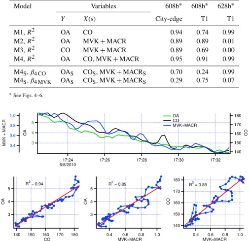
At this point the discussion shifts to the Sacramento plume proper, which consists of 56 transects on legs T0, City-Edge, T1, and Foothills. Coefficients of determination are shown for T1 transects in Fig. 3 (and repeated as part of Figs. S1– S3). In most cases, especially ones in which a high fraction of the OA spatial variability can be explained, more of the OA variance is explained by CO than by a biogenic tracer. According to the average values of R2 given in Table 5, adding the explanatory variable isoprene, MVK+MACR,
or CH3OH to M1, causesR2 to increase by 4, 7, or 13 %,
respectively. Standardized regression coefficients in Table 5 confirm the importance of CO and show that of the three bio-genic tracers, OA is best described by CH3OH.
Examples of time series for CO, MVK+MACR, and OA
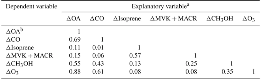
for three plumes are given in Figs. 4 to 6. Coefficients of determination for models M1–M4 and standardized regres-sion slopes for models M4S are provided in Table 6. In the
first two plumes from flight 608b (Figs. 4 and 5) OA is well correlated with both CO and MVK+MACR and the
two explanatory variables are themselves highly correlated. Small differences determine whether OA either follows CO or MVK+MACR more in the bilinear model, M4. In the third case from flight 628b (Fig. 6), OA is almost perfectly correlated with CO and there is an absence of correlation with MVK+MACR. Transects were not long enough to
fully observe both sides of a plume. Coverage was, however, usually more complete than the examples in Figs. 4 to 6.
1.0
0.8
0.6
0.4
0.2
0.0
Average R
2
Upwind T0 City-Edge T1 Foothills
OA Bi-linear (M4) OA vs CO (M1) OA vs Isoprene (M2) CO vs Isoprene (M3)
(a)
1.0
0.8
0.6
0.4
0.2
0.0
Average R
2
Upwind T0 City-Edge T1 Foothills
OA Bi-linear OA vs CO
OA vs MVK+MACR CO vs MVK+MACR
(b)
1.0
0.8
0.6
0.4
0.2
0.0
Average R
2
Upwind T0 City-Edge T1 Foothills
OA Bi-linear OA vs CO OA vs CH3OH CO vs CH3OH
(c)
Figure 2.Average coefficient of determination (R2)for bilinear or linear least-squares regressions using data from five locations for
plume transects shown in Fig. 1. Explanatory variables are(a)CO
and isoprene,(b)CO and MVK+MACR, and(c)CO and CH3OH.
Panel(a)gives regression model in parenthesis.
4.2 Regression analysis of plume perturbations
Correlations have also been calculated amongst plume per-turbation concentrations, defined for each transect as the 90th percentile minus the 10th percentile, and denoted here by the symbol1. While correlations on individual transects are only sensitive to cross-plume spatial variations, the correla-tions between1quantities test how well plume perturbations in OA follow perturbations in CO, MVK+MACR, isoprene, CH3OH, and O3, as these compounds vary in concentration
according to position (i.e., T0 to Foothills) and according to day-to-day variations in meteorological conditions. Table 7 summarizes values ofR2for linear regressions of all pairings of 1OA, 1CO, 1MVK+MACR, 1Isoprene, 1CH3OH,
and1O3. Also included are regression slopes andR2for the
vari-1.0
0.8
0.6
0.4
0.2
0.0
R
2
628b 628b 615b 624a 628a 608b 624b 615b 627a 608b 623b 619a 623b 624b 615a 608a 606a
T1 OA Bi-linear (M4)
OA vs CO (M1) OA vs isoprene (M2) CO vs isoprene (M3) (a)
1.0
0.8
0.6
0.4
0.2
0.0
R
2
628b 615b 628b 608b 624a 628a 608b 615b 627a 624b 615a 623b 619a 623b 624b 608a 606a
T1 (b) MVK+MACR
1.0
0.8
0.6
0.4
0.2
0.0
R
2
628b 615b 608b 624a 628b 628a 608b 627a 615b 624b 623b 623b 615a 619a 606a 624b 608a
T1 (c) CH3OH
Figure 3. Coefficient of determination (R2) for transects on
Leg T1, using CO as an anthropogenic tracer and (a) isoprene,
(b)MVK+MACR, and(c)CH3OH as a biogenic tracer. Results
rank ordered according to R2 of bilinear model, M4-Bio. Open
green circles indicates transects in which OA is anti-correlated with
Bio. Legend in panel(a)identifies regression models.
able1isoprene,1MVK+MACR, or1CH3OH to1OA vs.
1CO increases the explained variance from 69 to 76, 72 or 76 %, respectively. For independent transects, increases inR2 are significant with apvalue of 0.02 or better.
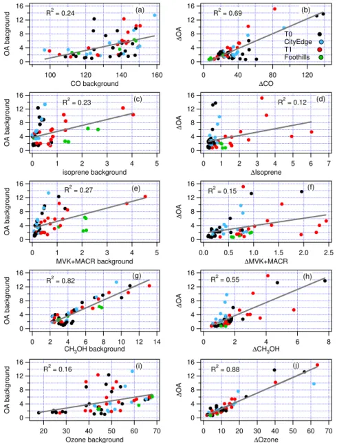
The inter-plume correlation analysis was repeated using background (10th percentile) values in place of 1s. Fig-ure 7 shows scatter plots for background OA vs. background CO, MVK+MACR, isoprene, and O3, paired with the
cor-responding scatter plots for 1 variables. Plots of 1 vari-ables correspond to the first column of data in Table 7. Color coding identifies points according to transect location. Background OA is poorly correlated with other background species, with the exception of OA vs. CH3OH (R2=0.82).
In that case there is a similar relation and goodness of fit for transects at all locations. The poor correlation between
back-Table 5.Coefficients of determination for models M1–M5, where
Bio is isoprene, MVK+MACR, or CH3OH, applied to
within-transect data. Average determined for 56 within-transects.
Modela Variables averageR2
Y X(s)
M1 OA CO 0.68
M2-isoprene OA isoprene 0.16
M3-isoprene CO isoprene 0.18
M4-isopreneb OA CO, isoprene 0.71
M2-MVK+MACR OA MVK+MACR 0.40
M3-MVK+MACR CO MVK+MACR 0.47
M4-MVK+MACRc OA CO, MVK+MACR 0.73
M2-CH3OH OA CH3OH 0.42
M3-CH3OH CO CH3OH 0.32
M4-CH3OHd OA CO, CH3OH 0.77
M5 OA O3 0.57
aWithin a set of regressions, M1 to M4, missing values of either OA, CO, or biogenic tracer were treated by removing all three data (listwise deletion).bAverage of standardized regression slopes for model M4-isopreneS,β4 CO=0.80,
β4 ISOPRENE= −0.01.cAverage of standardized regression slopes for model M4-MVK+MACRS,β4 CO=0.74,β4 MVK=0.06.dAverage of standardized regression slopes for model M4-CH3OHS,β4 CO=0.67,β4 CH3OH=0.29.
ground OA and CO is surprising in view of model results that show the Bay Area to be an important source region (Fast et al., 2012). Amongst the1variables,1OA has the high-est correlation with1O3(R2=0.88). Similar to the
within-transect spatial correlations, the variance of OA is better de-scribed by the anthropogenic tracer, CO (R2=0.69), than by a biogenic tracer.
4.3 Comparisons of low- and high-concentration transects
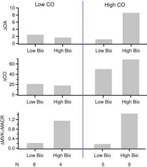
A third way of looking at OA as a function of anthropogenic and biogenic tracers is to divide the 56 transects into subsets according to tracer mixing ratio (Setyan et al., 2012; Shilling et al., 2013). Following Shilling et al. (2013), we have parsed our data into subsets according to whether mixing ratios of anthropogenic and biogenic tracers are low or high, defined here as being in the bottom or top third of their ranked distri-bution. Average concentrations of1OA were determined for the four combinations of low and high1CO and1Bio, with Bio being isoprene, MVK+MACR, or CH3OH.
Average concentrations for the1OA,1CO,1Bio systems are shown in Figs. 8–10. In the case of MVK+MACR, the nine samples that simultaneously have a high mixing ratio of 1CO and1MVK+MACR (high–high subset) have an
av-erage1OA=8.6 µg m−3 (Fig. 9). In contrast, subsets
hav-ing a low mixhav-ing ratio of either1CO and1MVK+MACR
or both have a low average1OA (1.1 to 2.4 µg m−3). Data subsets defined with1isoprene or1CH3OH share the
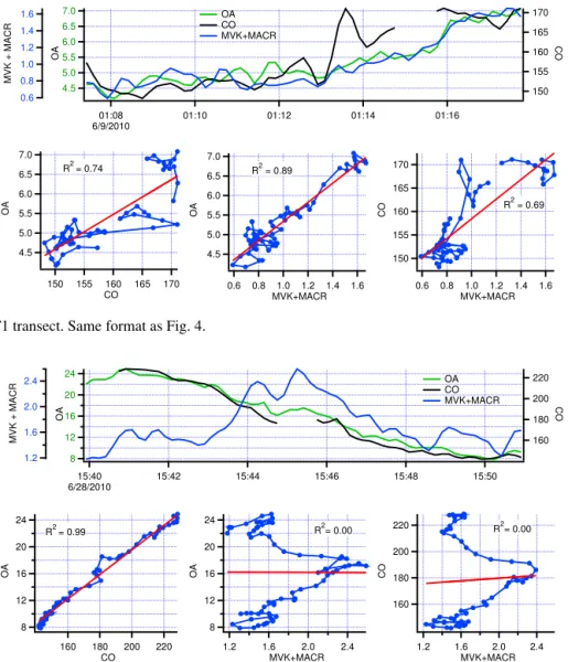
Table 6.Coefficients of determination for models M1–M4 and standardized regression slopes for model M4Sfor three transects.
Model Variables 608b∗ 608b∗ 628b∗
Y X(s) City-edge T1 T1
M1,R2 OA CO 0.94 0.74 0.99
M2,R2 OA MVK+MACR 0.89 0.89 0.01
M3,R2 CO MVK+MACR 0.89 0.69 0.00
M4,R2 OA CO, MVK+MACR 0.95 0.91 0.99
M4S,β4 CO OAS COS, MVK+MACRS 0.70 0.24 0.99
M4S,β4 MVK OAS COS, MVK+MACRS 0.29 0.75 0.07
∗See Figs. 4–6.
5
4
3
OA
17:24 6/8/2010
17:26 17:28 17:30 17:32
180
170
160
150
140
CO
1.0
0.8
0.6
0.4
MVK + MACR
OA CO MVK+MACR
5
4
3
OA
180 170 160 150 140
CO R2= 0.94
5
4
3
OA
1.0 0.8 0.6 0.4
MVK+MACR
R2 = 0.89 180
170
160
150
140
CO
1.0 0.8 0.6 0.4
MVK+MACR R2 = 0.89
Figure 4.Flight 608b City-Edge transect. Top graph: time series of OA, CO, and MVK+MACR. OA in µg m−3; CO and MVK+MACR in ppbv. Time is Pacific Standard Time. Bottom plots: correspond from left to right to models M1, M2, and M3 listwise deletion used for correlations but not used for graphs. Data points on scatter plots connected to give a sense of time continuity. Red lines are least-squares fit to data.
Figs. 8–10 that a component of the elevated 1OA in the high–high subset might be due to the subset having an ele-vated mixing ratio of anthropogenic and/or biogenic precur-sors (i.e., the high–high subset has more CO than the low-Bio–high-CO subset and more Bio than the low-CO–high-Bio subset). If A–B interactions did not exist, then by defi-nition1OA would respond independently to changes in an-thropogenic and biogenic precursors. We assume that the re-sponse would be linear. For each choice of1Bio, a bilinear model (M4) was applied to a set of transects that did not in-clude those in the high–high subset. The resulting intercept and slopes were used to calculate1OA for all transects. Ob-served and calculated values of1OA are shown in Fig. 11. In this approach, an A–B synergism should show up as a model under-prediction for the high–high subset. Indeed, there is an under-prediction of 1OA in the high–high subset but it is smaller than suggested by comparing1OA amongst sub-sets in Figs. 8–10. The ratio,1OA(observed)/ 1OA(bilinear model) for the high–high subset is 1.2 (0.3), 1.5 (0.3), and 1.2 (0.3), for isoprene, MVK+MACR, and CH3OH,
respec-tively. Numbers in parentheses are normalized root mean square deviations, a measure of the spread in A–B enhance-ments extracted from the high–high subset points in Fig. 11. Using only the averaged parsed data in Figs. 8–10 to remove precursor effects (see Fig. 8 caption) yields an A–B interac-tion factor of 1.5, 3.6, and 1.3 for isoprene, MVK+MACR, and CH3OH, respectively, closer to the results of Setyan et
al. (2012) and Shilling et al. (2013). Note that the choice of data subset used for the low concentration bilinear fit will ef-fect the calculated enhancements and may contribute to dif-ferences between values determined here and published val-ues.
5 Discussion
7.0
6.5 6.0
5.5
5.0 4.5
OA
01:08 6/9/2010
01:10 01:12 01:14 01:16
170
165
160
155
150
CO
1.6
1.4
1.2
1.0
0.8
0.6
MVK + MACR
OA CO MVK+MACR
7.0
6.5
6.0
5.5
5.0
4.5
OA
170 165 160 155 150
CO R2= 0.74
7.0
6.5
6.0
5.5
5.0
4.5
OA
1.6 1.4 1.2 1.0 0.8 0.6
MVK+MACR
R2 = 0.89 170
165
160
155
150
CO
1.6 1.4 1.2 1.0 0.8 0.6
MVK+MACR R2 = 0.69
Figure 5.Flight 608b T1 transect. Same format as Fig. 4.
24
20
16
12
8
OA
15:40 6/28/2010
15:42 15:44 15:46 15:48 15:50
220
200
180
160
CO
2.4
2.0
1.6
1.2
MVK + MACR
OA CO MVK+MACR
24
20
16
12
8
OA
220 200 180 160
CO R2= 0.99
24
20
16
12
8
OA
2.4 2.0 1.6 1.2
MVK+MACR
R2= 0.00 220
200
180
160
CO
2.4 2.0 1.6 1.2
MVK+MACR R2= 0.00
Figure 6.Flight 628b T1 transect. Same format as Fig. 4.
βs in model M4S, indicate that the explained variance is not
spurious. By these criteria the average dependence of OA on CO is greater than its dependence on the biogenic tracer CH3OH, and much greater than its dependence on isoprene
or MVK+MACR.
Although, on average, most of the explained variance in OA is due to CO, there are transects in which OA is highly correlated with isoprene, MVK+MACR or CH3OH
(Figs. 3, S1–S3). Examples for MVK+MACR are the
sequential-in-time City-Edge and T1 transects from the 608b flight shown in Figs. 4 and 5. Complicating the interpreta-tion of method 1 in general and the 608a transects in par-ticular, is the circumstance that the anthropogenic and bio-genic tracers, CO and MVK+MACR, are themselves often
highly correlated. As can be seen by comparing the standard-ized coefficients in Table 6 with values of R2 for models M1–M4, small difference in correlation coefficients can be associated with large changes in the relative importance of
CO and MVK+MACR as judged by the standardized
re-gression slopes. By most measures an R2 of 0.89 for OA vs. MVK+MACR on the 608b City-Edge transect would be considered excellent. But, because of the slightly higherR2 for OA vs. CO (0.94) and the high correlation between CO and MVK+MACR (0.89), a bilinear model assigns most of the variance in OA to CO. An opposite conclusion is reached for the 608b, T1 transect.
The spatial correlation between CO and, for example, MVK+MACR on individual transects is highly variable
(Figs. 3b and S2). On average it is somewhat greater than the correlation between OA and MVK+MACR. It is not
oxida-Table 7.Coefficients of determination between plume1avalues for OA, CO, isoprene, MVK+MACR, CH3OH, and O3based on data set of 56 transects.
Dependent variable Explanatory variablea
1OA 1CO 1Isoprene 1MVK+MACR 1CH3OH 1O3
1OAb 1
1CO 0.69 1
1Isoprene 0.11 0.01 1
1MVK+MACR 0.15 0.06 0.57 1
1CH3OH 0.55 0.43 0.13 0.25 1
1O3 0.88 0.61 0.08 0.08 0.35 1
a1defined for each transect as the 90th percentile of concentration–10th percentile.bBilinear regression with standardized
variables:
1OAS=β41CO1COS+β41IOPRENE1IsopreneS:β41CO=0.80,β41ISOPRENE=0.26,R2=0.76.
1OAS=β41CO1COS+β41MVK1MVK+MACRS:β41CO=0.78,β41MVK=0.19,R2=0.72.
1OAS=β41CO1COS+β41CH3OH1CH3OHS:β41CO=0.60,β41CH3OH=0.35,R2=0.76.
tion of isoprene in the high NOx anthropogenic Sacramento
plume could be a contributing factor. Perhaps related is the observation by Dreyfus et al. (2002) of the co-advection of anthropogenic and biogenic compounds from the direction of Sacramento to the Blodgett Forest Research Station.
In Method 2, plume perturbations (1s) are defined on each downwind transect and for each species of interest. Corre-lation coefficients calculated amongst transects quantify the extent to which linear and bilinear combinations of 1 trac-ers (CO, isoprene, MVK+MACR, CH3OH, and O3) can explain the variations of 1OA that occur as chemical and meteorological conditions vary from flight to flight and with transect location. As with method 1, we find that CO is more successful in explaining the variability of OA, in comparison to biogenic tracers. This can be seen from the scatter dia-grams in Fig. 7 and from the standardized coefficients for the bilinear model M4Sin Table 7.
A notable feature of the correlations amongst transects is that 1O3 explains 88 % of the variance in1OA. A display
of Fig. 7j on a log–log scale (not shown) indicates that the 1OA–1O3relation stays approximately constant at low
con-centrations. Figure 7j also shows that the same relation holds at each of the four downwind transect locations. The high 1OA–1O3correlation is evidence that most OA above
back-ground originates from secondary chemistry. This assign-ment is in agreeassign-ment with findings from many locations that SOA is correlated with other oxidized species and in agree-ment with the analysis of CARES observations by Setyan et al. (2012) and Shilling et al. (2013). A mechanistic reason for a relation between OA and O3 was proposed by
Hern-don et al. (2008) based on a chemical mechanism in which OH+VOC was the rate limiting step in O3production, and
also in forming low volatility VOC oxidation products that partition to the aerosol phase. The least-squares fit in Fig. 7j has a slope of 225 µg m−3 per ppm O
3, as compared with
the 104–180 µg m−3per ppm O
3slopes found by Herndon et
al. (2008) in Mexico City outflow. Differences could reflect
a±30 % uncertainty in AMS measurements (Canagaratna et
al., 2007) or variations in processing conditions.
Because of the mismatch in atmospheric lifetimes be-tween isoprene or MVK+MACR and OA, it is not clear whether a correlation should be expected. Shilling et al. (2013) have made an argument based on changes be-tween pseudo Lagrangian morning and afternoon measure-ments, that an anti-correlation is consistent with OA for-mation from biogenics that have been depleted by oxi-dation reactions. Robust relations between SOA and bio-genic tracers are typically not found. For example, de Gouw et al. (2005) present aerosol and trace gas measurements from the Ronald H. Brown, taken off the coast of a re-gion in Maine with high biogenic emission rates. Sub-µm OA was observed to be highly correlated with the anthro-pogenic tracer, iso-propyl nitrate, but not correlated with either monoterpenes or isoprene. A similar lack of corre-lation was found by Sullivan et al. (2006) and Weber et al. (2007). In contrast, Slowik et al. (2010) showed an R2 of 0.71 for a regression of less oxygenated SOA (OOA-2; O/C=0.46) vs. MVK+MACR, concluding on the basis of the MVK+MACR lifetime that OOA-2 was formed in the
relatively recent past. Setyan et al. (2012) also observed a high correlation (R2=0.61) between MVK+MACR and a
more-oxidized OOA (O/C=0.54) at T1.
Unlike isoprene and MVK+MACR, the atmospheric
life-time of CH3OH is comparable to that of SOA.
Standard-ized regression coefficients averaged over all transects (Ta-ble 5) indicate that CH3OH captures the spatial variance in
16 12 8 4 0 OA bacground 160 140 120 100 CO background (a)
R2 = 0.24
16 12 8 4 0 D OA 120 80 40 0 DCO T0 CityEdge T1 Foothills (b)
R2 = 0.69
16 12 8 4 0 OA background 5 4 3 2 1 0 isoprene background (c)
R2 = 0.23
16 12 8 4 0 D OA 7 6 5 4 3 2 1 0 DIsoprene (d)
R2 = 0.12
16 12 8 4 0 OA background 5 4 3 2 1 0 MVK+MACR background (e)
R2 = 0.27 16
12 8 4 0 D OA 2.5 2.0 1.5 1.0 0.5 0.0 DMVK+MACR (f)
R2 = 0.15
16 12 8 4 0 OA background 14 12 10 8 6 4 2 0
CH3OH background
(g)
R2 = 0.82
16 12 8 4 0 D OA 8 6 4 2 0
DCH3OH
(h)
R2 = 0.55
16 12 8 4 0 OA background 70 60 50 40 30 20 Ozone background (i)
R2 = 0.16
16 12 8 4 0 D OA 70 60 50 40 30 20 10 0 DOzone (j)
R2 = 0.88
Figure 7.OA as a function of CO, isoprene, MVK+MACR, CH3OH, and O3for 56 transects. Background concentrations in panels on
left-hand side;1Concentrations on the right-hand side. Color legend in panel(b)identifies data according to location. Gray lines are linear
least-squares fits withR2given in each panel.
Figure 7 shows that the variance in background OA is uniquely captured by background CH3OH, with an explained
variance of 82 % compared to 23 to 27 % for background CO, isoprene, or MVK+MACR. The excellent fit between
back-ground OA and backback-ground CH3OH and the poor fit with CO
is what would be expected if background SOA is primarily biogenic.
In method 3, concentrations in the form of 1 val-ues are used to define plume-transect subsets, which have low or high mixing ratios of CO and either isoprene, MVK+MACR, or CH3OH. Of the four combinations of low
and high values of1CO and 1Bio, only the subset with a high mixing ratio of both anthropogenic and biogenic trac-ers has high average1OA. However, according to method 1,
most transects have a correlation between OA and biogenic tracers that is low and/or spurious, such that the addition of a biogenic to an OA vs. CO model, produces only a mod-est improvement in explaining the variance of OA during a plume transect. In method 2, there is a poor correlation be-tween1OA and1isoprene or1MVK+MACR. The
cor-relation between 1OA and 1CH3OH is somewhat higher
but still lower than that between1OA and 1CO. We rec-ognize the deficiencies in using short-lived biogenic tracers, yet in method 3 these same biogenic tracers as well as the long-lived CH3OH can split the data set into subsets with
and without high1OA.
heav-10 8 6 4 2 0
∆
OA
Low Bio High Bio Low Bio High Bio
60
40
20
0
∆
CO
Low Bio High Bio Low Bio High Bio
4
3
2
1
0
∆
Isoprene
Low Bio High Bio Low Bio High Bio
Low CO High CO
N 6 6 7 6
Figure 8.Values of1OA,1CO, and1Isoprene for 4 subsets of
transects. Pairs of bars labeled low CO and high CO have1CO
val-ues that are below the 33rd percentile and above the 67th percentile,
respectively. Bars labeled low Bio and high Bio have 1Isoprene
values that are below the 33rd percentile and above the 67th per-centile, respectively. Number of transects in each subset given at
bottom.1CO ratio and1Bio ratio give effects of precursor mixing
ratio on an A–B interaction relative to the expectation that1OA is
a bilinear function of1CO, and1Bio:1CO ratio is (1CO: high
CO, high Bio)/(1CO: high CO, low Bio).1Bio ratio is (1Bio:
high CO, high Bio)/(1Bio: high CO, low Bio).
10 8 6 4 2 0
∆
OA
Low Bio High Bio Low Bio High Bio
60
40
20
0
∆
CO
Low Bio High Bio Low Bio High Bio
1.2
0.8
0.4
0.0
∆
MVK+MACR
Low Bio High Bio Low Bio High Bio
Low CO High CO
N 8 4 5 9
Figure 9.Bar graphs for subsets defined on the basis of1CO and
1MVK+MACR. Same format as Fig. 8.
10 8 6 4 2 0
∆
OA
Low Bio High Bio Low Bio High Bio
80
60
40
20
0
∆
CO
Low Bio High Bio Low Bio High Bio
4
3
2
1
0
∆
CH
3
OH
Low Bio High Bio Low Bio High Bio
Low CO High CO
N 8 5 5 8
Figure 10.Bar graphs for subsets defined on the basis of1CO and
1CH3OH. Same format as Fig. 8.
ily reliant on data from two flights on 28 June as this was the only day in which1OA exceeded 6 µg m−3. What was dis-tinctive about this day? According to Fast et al. (2012), from 22 June till the end of the field campaign on 28 June, winds at 700 hPa were light and variable. After 25 June there was a steady increase in maximum day time temperature; 27 and 28 June had the warmest temperatures, approaching 40◦C
at T0 on the 28th. Ozone also reached its highest value of 90 ppb at T0. Wind speeds at the G-1 altitude were∼2 m s−1.
A detailed description of chemical conditions on 28 June is given by Shilling et al. (2013). In brief, during these two flights isoprene reached 13 ppb, O3approached 120 ppb, CO
was in excess of 260 ppb, and OA more than 25 µg m−3. Ex-cept for CO, these values are the highest observed from the G-1 during CARES.
16
12
8
4
0
D
OA
50 40 30 20 10 0
Observed Bi-linear fit High Anthro, Bio
CO Isoprene
16
12
8
4
0
D
OA
50 40 30 20 10 0
Observed Bi-linear fit High Anthro, Bio
CO MVK+MACR
16
12
8
4
0
D
OA
50 40 30 20 10 0
Transects
Observed Bi-linear fit High Anthro, Bio
CO Methanol
Figure 11. Observed 1OA presented in descending order. Blue
trace is 1OA from bilinear model using1CO and(a)Isoprene,
(b)1MVK+MACR, and(c)1CH3OH as explanatory variables.
Regressions did not use transects from the high1CO, high1Bio
subsets, indicated by red symbols.
28 June. The driving meteorological factors, however, do not necessarily affect OA and OA precursors equally, with the result that trends in the parsed data can exist without strong correlations between1OA and1Bio.
According to our definition of plume perturbations (1s) approximately 60 % of peak OA in the Sacramento plume is background. This value is determined by a 56 transect aver-age of the ratio OA(10th percentile)/OA (90th percentile). A high contribution from background is consistent with trans-port simulations retrans-ported by Fast et al. (2012). As back-ground SOA would be aged, its presence is consistent with the O to C ratios reported by Shilling et al. (2013). Correla-tions between background OA and its precursors, in particu-lar the strong correlation with background CH3OH and weak
correlation with background CO, suggest that background OA is primarily biogenic. Background aerosol will foster the formation of OA in the Sacramento plume by more than dou-bling the aerosol volume potentially available for gas to par-ticle partitioning. The increase in partitioning realized will depend on the volatility of gas phase precursors and aerosol viscosity and phase (e.g., Zaveri et al., 2014; Madronich et al., 2015). In so far as isoprene and its oxidation products are expected to dominant VOC reactivity, these compounds will affect the processing of anthropogenic carbon and may be seen as contributing to A–B interactions.
The circumstance that∼60 % of peak OA is background, and appears to be primarily biogenic, has the consequence that the fraction of non-fossil carbon in the Sacramento plume will be significantly greater than half, especially since plume OA is partially biogenic and approximately 20–30 % of urban anthropogenic emissions are estimated to be from non-fossil sources, such as cooking, trash burning, and bio-fuel use (Hodzic et al., 2011; Zotter et al., 2014). There were no14C measurements to compare with our correlation-based predictions, but given observations in areas with lower bio-genic emission rates (Marley et al., 2009), and given observa-tions made at Blodgett Forest (Worton et al., 2011), it would be surprising if non-fossil carbon did not predominate.
6 Conclusions
We have used aircraft observations obtained during the CARES field campaign to infer whether background OA and OA produced in the Sacramento plume are primarily anthro-pogenic or biogenic, whether there is enhanced OA forma-tion caused by interacforma-tions between anthropogenic and bio-genic compounds, and if observations are consistent with14C measurements from other locations. Linear and bilinear cor-relations for 56 individual transects show how well OA fol-lows explanatory variables over small spatial scales, whilst correlations amongst transects yield information on how 1OA (plume perturbation) varies due to changes in location and day-to-day variations in meteorological conditions. Fol-lowing Setyan et al. (2012) and Shilling et al. (2013), tran-sects are split into subsets in order to determine whether high OA concentrations are uniquely associated with high mixing ratios of anthropogenic and biogenic tracers.
Explanatory variables were CO as a tracer of anthro-pogenic OA precursors and isoprene, MVK+MACR, and
CH3OH as tracers of biogenic emissions. In addition O3
was used as a surrogate for photochemical activity. Tracers should ideally have lifetimes comparable to the timescales over which OA is formed. CO is long lived. CH3OH is
used here (to the best of our knowledge, for the first time) as an analogous long-lived biogenic tracer with an atmo-spheric lifetime of ∼10 days. In contrast, isoprene and
MVK+MACR have lifetimes ranging from less than an hour
to a few hours. We have found that
correlations between OA and explanatory variables ne-cessitate the use of multivariate models.
3. The correlation between 1OA and 1O3 (R2=0.88)
agrees with the findings of Herndon et al. (2008) and Wood et al. (2010) that there is a common rate limit-ing step for production of O3and SOA within an urban
plume.
4. The excellent correlation between background OA and background CH3OH (R2=0.82) and the low
correla-tion with background CO (R2=0.24) is consistent with a biogenic origin for background OA. This compari-son requires a long-lived biogenic tracer as the mea-sured isoprene or MVK+MACR backgrounds are
un-likely to have been present when the background OA was formed. As such they show little correlation. 5. Background OA is on average 60 % of peak OA. On
the basis of background OA being primarily of biogenic origin and SOA formed downwind of Sacramento de-riving primarily from anthropogenic carbon, a fraction of which is non-fossil, it is predicted that OA found in the Sacramento plume would be mostly non-fossil. 6. Evidence for A–B interaction comes from comparing
1OA between data subsets having different combina-tions of low and high mixing ratios of anthropogenic and biogenic tracers. We are able to reproduce the find-ings of Setyan et al. (2012) and Shilling et al. (2013) that high values of OA only occur when anthropogenic and biogenic compounds both have a high mixing ratio. Differences in precursor abundance between data sub-sets should be taken into account to determine what por-tion of OA can be attributed to A–B interacpor-tions. Doing so by using residuals from a bilinear fit to the amongst transect data set, yields estimates that A–B interactions can increase OA concentration by a factor of 1.2 to 1.5 depending on the compound used as a tracer of biogenic emissions. This increase is relative to the bilinear rela-tion describing data not in the high CO–high Bio subset. A–B interactions up to a factor of 3.6 are obtained from a fit to coarser subset-averaged data.
7. The data subset with high values of anthropogenic and biogenic precursors is dominated by two flights on the last day of the field campaign. Temperature reached 40◦C and wind speed was ∼2 m s−1. Concentrations
of OA, O3, and biogenic trace gases were the highest
recorded, and CO was close to the highest recorded. In addition to the many mechanisms for A–B inter-actions described in the literature (e.g. Carlton et al., 2010; Hoyle et al., 2011; Xu et al., 2015) it is useful to consider whether additional mechanisms are enabled during a pollution episode such as what occurred on 28 June. Poor ventilation and high temperatures lead to increased biogenic emissions, higher ambient amounts
of biogenic and anthropogenic SOA precursors, and in-creased photochemical activity as evidenced by a higher O3 mixing ratio, the latter requiring the presence of
anthropogenic NOx. Thus, the highest SOA
concentra-tions are likely to occur coincident with elevated mixing ratios of both anthropogenic and biogenic tracers. By its very nature conclusions based on correlations are inferential. It would be highly desirable to test our results against a high-resolution chemical transport model. Model calculations are essential for comparisons between CARES and other regions; in particular, the well-studied eastern USA in which aerosols have higher relative and absolute amounts of inorganic constituents and there is a greater abundance of liquid water, perhaps enabling A–B mechanisms to a greater extent than observed in the CARES region.
Copyright statement
The author’s copyright for this publication is transferred to US Government.
The Supplement related to this article is available online at doi:10.5194/acp-16-1729-2016-supplement.
Acknowledgements. We thank chief pilot Bob Hannigan and the
flight crew from PNNL for a job well done. We gratefully ac-knowledge the Atmospheric Radiation Measurement (ARM) and the Atmospheric Systems Research (ASR) Programs within the Office of Biological and Environmental Research of the Office of Science of the US Department of Energy (DOE) for support-ing field and analysis activities and for providsupport-ing the G-1 aircraft. Support for J. Fast, J. Hubbe, J. Shilling, and R. Zaveri of Pa-cific Northwest National Laboratory and Q. Zhang of U. C. Davis was provided by the US DOE under contracts DE-A06-76RLO 1830 and DE-SC0007178, respectively. Research by L. Kleinman, C. Kuang, A. Sedlacek, G. Senum, S. Springston, and J. Wang of Brookhaven National Laboratory was performed under sponsorship of the US DOE under contracts DE-SC0012704.
This research was performed under the auspices of the United States Department of Energy under contract no. DE-SC0012704.
Edited by: G. McFiggans
References
Carlton, A. G. and Turpin, B. J.: Particle partitioning potential of organic compounds is highest in the Eastern US and driven by anthropogenic water, Atmos. Chem. Phys., 13, 10203–10214, doi:10.5194/acp-13-10203-2013, 2013.
Carlton, A. G., Wiedinmyer, C., and Kroll, J. H.: A review of Sec-ondary Organic Aerosol (SOA) formation from isoprene, At-mos. Chem. Phys., 9, 4987–5005, doi:10.5194/acp-9-4987-2009, 2009.
Carlton, A. G., Pinder, R. W., Bhave, P. V., and Pouliot, G. A.: To What Extent Can Biogenic SOA be Controlled?, Environ. Sci. Technol., 44, 3376–3380, doi:10.1021/es903506b, 2010. Chen, Q., Farmer, D. K., Schneider, J., Zorn, S. R., Heald, C. L.,
Farl, T. G., Guenther, A., Allan, J. D., Robinson, N., Coe, H., Kimmel, J. R., Pauliquevis, T., Borrmann, S., Pöschl, U., An-dreae, M. O., Artaxo, P., Jimenez, J. L., and Martin, S. T.: Mass spectral characterization of submicron biogenic organic parti-cles in the Amazon Basin, Geophys. Res. Lett., 36, L20806, doi:10.1029/2009GL039880, 2009.
de Gouw, J. and Jimenez, J. L.: Organic Aerosols in the Earth’s Atmosphere, Environ. Sci. Technol., 43, 7614–7618, 2009. de Gouw, J. A., Middlebrook, A. M., Warneke, C., Goldan, P.
D., Kuster, W. C., Roberts, J. M., Fehsenfeld, F. C., Worsnop, D. R., Canagaratna, M. R., Pszenny, A. A. P., Keene, W. C., Marchewka, M., Bertman, S. B., and Bates, T. S.: Budget of or-ganic carbon in a polluted atmosphere: Results from the New England Air Quality Study in 2002, J. Geophys. Res., 110, D16305, doi:10.1029/2004JD005623, 2005.
de Gouw, J. A., Brock, C. A., Atlas, E. L., Bates, T. S., Fehsen-feld, F. C., Goldan, P. D., Holloway, J. S., Kuster, W. C., Lerner, B. M., Matthew, B. M., Middlebrook, A. M., Onasch, T. B., Peltier, R. E., Quinn, P. K., Senff, C. J., Stohl, A., Sullivan, A. P., Trainer, M., Warneke, C., Weber, R. J., and Williams, E. J.: Sources of particulate matter in the northeastern United States in summer: 1.Direct emissions and secondary formation of organic matter in urban plumes, J. Geophys. Res.-Atmos., 113, D08301, doi:10.1029/2007jd009243, 2008.
Dreyfus, G. B., Schade, G. W., and Goldstein, A. H.: Observational constraints on the contribution of isoprene oxidation to ozone production on the western slope of the Sierra Nevada, California, J. Geophys. Res., 107, 4365, doi:10.1029/2001JD001490, 2002. Ervens, B., Turpin, B. J., and Weber, R. J.: Secondary or-ganic aerosol formation in cloud droplets and aqueous parti-cles (aqSOA): a review of laboratory, field and model stud-ies, Atmos. Chem. Phys., 11, 11069–11102, doi:10.5194/acp-11-11069-2011, 2011.
Fast, J. D., Gustafson Jr., W. I., Berg, L. K., Shaw, W. J., Pekour, M., Shrivastava, M., Barnard, J. C., Ferrare, R. A., Hostetler, C. A., Hair, J. A., Erickson, M., Jobson, B. T., Flowers, B., Dubey, M. K., Springston, S., Pierce, R. B., Dolislager, L., Ped-erson, J., and Zaveri, R. A.: Transport and mixing patterns over Central California during the carbonaceous aerosol and radiative effects study (CARES), Atmos. Chem. Phys., 12, 1759–1783, doi:10.5194/acp-12-1759-2012, 2012.
Goldstein, A. H., Koven, C. D., Heald, C. L., and Fung, I. Y.: Bio-genic carbon and anthropoBio-genic pollutants combine to form a cooling haze over the southeastern United States, P. Natl. Acad. Sci., 106, 8835–8840, 2009.
Guenther, A., Hewitt, C.N., Erickson, D., Fall, R., Geron, C., Graedel, T., Harley, P., Klinger, L., Lerdau, M., McKay, W. A.,
Pierce, T., Scholes, B., Steinbrecher, R., Tallamraju, R., Taylor, T., and Zimmerman, P.: A global model of natural volatile or-ganic compound emission, J. Geophys. Res., 100, 8873–8892, 1995.
Guenther, A. B., Zimmerman, P. R., Harley, P. C., Monson, R. K., and Fall, R.: Isoprene and monoterpene emission rate variability: Model evaluations and sensitivity analysis, J. Geophys. Res., 98, 12609–12617, 1993.
Herndon, S. C., Onasch, T. B., Wood, E. C., Kroll, J. H., Cana-garatna, M. R., Jayne, J. T., Zavala, M. A., Knighton, W. B., Maz-zoleni, C., Dubey, M. K., Ulbrich, I. M., Jimenez, J. L., Seila, R., de Gouw, J. A., de Foy, B., Fast, J., Molina, L. T., Kolb, C. E., and Worsnop, D. R.: Correlation of secondary organic aerosol with odd oxygen in Mexico City, Geophys. Res. Lett., 35, L15804, doi:10.1029/2008GL034058, 2008.
Hodzic, A., Jimenez, J. L., Prévôt, A. S. H., Szidat, S., Fast, J. D., and Madronich, S.: Can 3-D models explain the observed fractions of fossil and non-fossil carbon in and near Mexico City?, Atmos. Chem. Phys., 10, 10997–11016, doi:10.5194/acp-10-10997-2010, 2010.
Hoyle, C. R., Boy, M., Donahue, N. M., Fry, J. L., Glasius, M., Guenther, A., Hallar, A. G., Huff Hartz, K., Petters, M. D., Petäjä, T., Rosenoern, T., and Sullivan, A. P.: A review of the anthro-pogenic influence on biogenic secondary organic aerosol, Atmos. Chem. Phys., 11, 321–343, doi:10.5194/acp-11-321-2011, 2011. Kanakidou, M., Tsigaridis, K., Dentener, F. J., and Crutzen, P. J.: Human-activity enhanced formation of organic aerosols by bio-genic hydrocarbon oxidation, J. Geophys. Res., 105, 9243–9254, 2000.
Kleinman, L. I., Springston, S. R., Wang, J., Daum, P. H., Lee, Y.-N., Nunnermacker, L. J., Senum, G. I., Weinstein-Lloyd, J., Alexander, M. L., Hubbe, J., Ortega, J., Zaveri, R. A., Cana-garatna, M. R., and Jayne, J.: The time evolution of aerosol size distribution over the Mexico City plateau, Atmos. Chem. Phys., 9, 4261–4278, doi:10.5194/acp-9-4261-2009, 2009.
Lindinger, W., Hansel, A., and Jordan, A.: On-line monitoring of volatile organic compounds at pptv levels by means of proton transfer-reaction mass spectrometry (PTR-MS) – Medical appli-cations, food control and environmental research, Int. J. Mass Spectrom., 173, 191–241, 1998.
Madronich, S., Conley, A., Lee-Taylor, J., Kleinman, L., Hodzic, A., and Aumont, B.: Non-linear partitioning and organic volatility distributions of urban aerosols, Faraday Discuss., doi:10.1039/C5FD00209E, online first, 2015.
Marley, N. A., Gaffney, J. S., Tackett, M., Sturchio, N. C., Heraty, L., Martinez, N., Hardy, K. D., Marchany-Rivera, A., Guilderson, T., MacMillan, A., and Steelman, K.: The impact of biogenic car-bon sources on aerosol absorption in Mexico City, Atmos. Chem. Phys., 9, 1537–1549, doi:10.5194/acp-9-1537-2009, 2009. Matsui, H., Koike, M., Takegawa, N., Kondo, Y., Griffin, R. J.,
Miyazaki, Y., Yokouchi, Y., and Ohara, T.: Secondary Organic Aerosol Formation in Urban Air: Temporal Variations and Possi-ble Contributions from Unidentified Hydrocarbons, J. Geophys. Res.-Atmos., 114, D04201, doi:10.1029/2008JD010164, 2009. Ng, N. L., Kroll, J. H., Keywood, M. D., Bahreini, V. V., Flagan,